Lower bound on the proton charge radius from electron scattering data
Abstract
The proton charge-radius determinations from the electromagnetic form-factor measurements in electron-proton () scattering require an extrapolation to zero momentum transfer () which is prone to model-dependent assumptions. We show that the data at finite momentum transfer can be used to establish a rigorous lower bound on the proton charge radius. Using the available data at low (below 0.02 GeV2), we obtain fm (with 95% confidence) as the lower bound on the proton radius. This result takes into account the statistical errors of the experiment, whereas the systematic errors are assumed to contribute to the overall normalization of the cross section only. With this caveat in mind, the obtained lower bound is on the edge of reaffirming the discrepancy between the and muonic-hydrogen values, while bypassing the model-dependent assumptions that go into the fitting and extrapolation of the data. The near-future precise experiments at very low , such as PRad, are expected to set a more stringent bound.
Keywords:
Charge radius , proton size , form factors , charge distribution , electron scattering1 Introduction
The proton charge radius is traditionally accessed in elastic electron-proton () scattering at small momentum transfers (low ) Hofstadter and McAllister 1955, Hofstadter 1957. Recently, however, the accuracy of this method has been questioned in the context of the proton-radius puzzle, which is partially attributed to the discrepancy between the 2010 scattering value of Bernauer et al. Bernauer et al. 2010, Bernauer et al. 2014 and the muonic-hydrogen (H) extraction of the proton radius Pohl et al. 2010, Antognini et al. 2013, see Fig. 1. Meanwhile, as seen from the figure, the different extractions based on -scattering data have covered a whole range of values and hardly add-up into a coherent picture.
A “weak link” of the proton-radius extractions from experiments is the extrapolation to zero momentum transfer. Namely, while the data taken in some finite- range can directly be mapped into the proton (electric and magnetic) Sachs form factors and , the radii extractions require the derivatives of those at , e.g.: . As much as one believes that the slope at is largely determined by the behavior at finite , it is not easy to quantify this relation with the necessary precision. The issues of fitting and extrapolation of the form-factor data have lately been under intense discussion, see, e.g., Refs. Sick 2012, Bernauer 2016, Hayward and Griffioen 2018, Yan et al. 2018. Similar extrapolation problems should exist in the extractions based on lattice QCD, since the lowest momentum-transfer therein is severely limited by the finite volume.
Here, we show that the form-factor data at finite provide a lower bound on the proton charge radius. A determination of this bound needs no extrapolation, therefore no major model assumptions, and should be based solely on experimental (or lattice) data. At the same time, given that some of the conventional extractions from data show a considerably larger radius than the H value, a strict lower bound, based purely on data, is potentially useful in understanding this discrepancy.
In what follows, we briefly recall the basic formulae in Sec. 2, introduce the quantity proposed to serve as the charge-radius bound in Sec. 3, obtain an empirical value for it based on proton electric form-factor data in Sec. 4 and conclude in Sec. 5.
2 Basic ingredients of the radius extraction
Let us recall that a spin-1/2 particle, such as the proton, has two electromagnetic form factors. These are either the Dirac and Pauli form factors: and ; or, the electric and magnetic Sachs form factors:
| (1a) | |||||
| (1b) | |||||
with the particle mass. The Sachs form factors can be interpreted as the Fourier transforms of the charge and magnetization distributions, and , in the Breit frame. Strictly speaking, this relation holds only for spherically symmetric densities, in which case one has, see e.g. Ref. Perdrisat et al. 2007:
| (2a) | |||||
| (2b) | |||||
where is the spherical Bessel function, and is the anomalous magnetic moment of the proton. Note that these are Lorentz-invariant expressions, hence, the spherically symmetric charge and magnetization distributions are, just as the form factors, Lorentz-invariant quantities.
The radii are introduced through the density moments, which, for even , can be given by the form-factor derivatives at :
| (3) | |||||
and similarly for the magnetic radii with replaced by , and replaced by , respectively. Therefore, the Taylor expansion of the form factor around is written as:
| (4) | |||||
The subject of interest is the root-mean-square (rms) radius (or, simply the charge radius): . Ideally, it could be extracted by fitting the first few terms of the above Taylor expansion of the form factor to the experimental data at low . In practice, however, this does not work. The main reason is that the convergence radius of the Taylor expansion is limited by the onset of the pion-production branch cut for time-like photon momenta at (the nearest singularity, as far as the strong interaction is concerned), and there are simply not many data for GeV2.
A viable approach to fit to higher is, instead of the Taylor expansion, to use a form which takes the singularities into account. This is done in the -expansion Hill and Paz 2010 and dispersive fits Adamuscin et al. 2012, Lorenz et al. 2015, Alarcón et al. 2018. These approaches have, however, other severe limitations. The -expansion only deals with the first singularity and therefore extends the convergence radius to only. The dispersive approach is based on an exact dispersion relation for the form factor:
| (5) |
which, in principle, accounts for all singularities. Unfortunately, it requires the knowledge of the spectral function, , which is not directly accessible in experiment, and needs to be modeled. Chiral perturbation theory can only provide a description of this function in the range of GeV2. Despite the recent progress in the empirical description of the spectral function Hoferichter et al. 2016, the problem of model dependence of the radius extraction in the dispersive approach remains to be non-trivial.
3 Positivity bounds
Given the aforementioned issues in extracting the charge radius from form-factor data, we turn to establishing a bound on the radius, rather than the radius itself. The advantage is that the bound will follow from the finite- data alone and needs no extrapolations or model assumptions.
To this end we consider the following quantity:
| (6) |
which in the real-photon limit yields the radius squared:
| (7) |
As will be argued in Sec. 3, the spacelike () proton form factor is bounded from above:
| (8) |
and hence, the above log-function is positive, . Furthermore, if falls with increasing not faster than by a power law, then falls as well. The analytic properties of , in the absence of zeros, are inherited by its logarithm. The subtracted dispersion relation (5) for the form factor then leads to an unsubtracted one for :
| (9) |
where , and is the phase defined through . This dispersion relation shows that the function is monotonic in the spacelike region. The latter allows one to establish a lower bound on the radius:
| (10) |
Substituting in here the Taylor expansion, Eq. (4), one has:
| (11) |
and so, in order for the bound to hold at arbitrarily low , the fourth and second moments must satisfy the following inequality:11 1 Based on Eq. (9), one can claim that is completely monotonic, i.e.: , from which the lower bounds on other radii can be derived. The lowest values of the radii are given in terms of the charge radius , and can all be obtained from Taylor-expanding the following form of the form factor: .
| (12) |
We have checked that this non-trivial hierarchical condition on the radii, which follows from the lower bound Eq. (10), is verified in existing empirical parametrizations of the proton form factor, of which the dipole form, , is the simplest one.
The fact that is monotonically increasing towards means that the best bound is obtained at lowest accessible . In practice, however, it depends on the size of the experimental errors, including the uncertainty in the overall normalization of the form factor. We discuss this in detail in Sec. 4, when obtaining the empirical value of the bound from experimental data. In the rest of this section we focus on the proof of Eq. (8).

The unitary bound on the proton form factor, given in Eq. (8), and subsequently the radius bound, given in Eq. (10), follow from positivity of the corresponding charge density distribution: . Indeed, from Eq. (2a),
| (13) |
with the property of the Bessel function , and the positivity of , we can see see that the integrand on the right-hand side is positive definite, and Eq. (8) follows upon substituting on the left-hand side.
There is a concern Miller 2010 that the proton charge density is not necessarily positive definite, and only the transverse charge density is (). The latter relates to the Dirac form factor through the two-dimensional Fourier transform:
| (14) |
where is the cylindrical Bessel function. However, the positivity of the transverse charge density is sufficient to prove the unity bound of Eq. (8). To see this, one may apply the previous argument [cf. Eq. (13)] to Eq. (14) using , and derive the bound on the Dirac form factor:
| (15) |
Then, the unitary bound on follows from its definition in terms of the Dirac and Pauli form factors, see Eq. (1a), by taking into account the conditions and . The latter is valid for the proton in at least the low- region, as can be seen empirically from , with the anomalous magnetic moment of the proton.
While the unity bound on follows from the positivity of , the reverse is not necessarily true. Therefore, the proof based on the positivity of the transverse charge density does not necessarily imply the positivity of . Introducing as the three-dimensional Fourier-transform of the Dirac form factor, we have:
| (16) |
and matching it to Eq. (14), we obtain its relation to the transverse density:22 2 Here we recall the following relations between the spherical and cylindrical Bessel functions: as well as their orthogonality:
| (17a) | |||||
| (17b) | |||||
The two are thus related by the Abel transform [Bracewell 2000, p. 351 et seqq.]. It infers , for , while the reverse is not necessarily true.
4 Exploring the scattering data
4.1 Direct determination
We now proceed to obtaining the lower bound on the proton charge radius from scattering data. The first step is to convert the experimental data for to , using the definition (6). The presently available data in the region well below the pion-pair production scale (here we chose GeV2) are shown in Fig. 2. The light-blue points are from the dataset of Bernauer et al. Bernauer et al. 2010, Bernauer et al. 2014. The light-red data points are from the recent initial-state radiation (ISR) experiment at MAMI Mihovilović et al. 2017. In both cases we deal with the statistical error bars only. The two points at indicate the muonic-hydrogen (green) and Bernauer’s -scattering (dark-blue) values of the proton charge radius.
In principle, every data point in Fig. 2, at finite , provides a lower bound on the proton charge radius. For a more accurate value, we can average over any subset of these data. In the figure, the horizontal blue band is the statistical average of Bernauer’s dataset, whereas the red band is the statistical average of the ISR dataset. The corresponding values for the lower bound are presented in the “Raw-average” column of Table 1.
This is how ideally the bound should be determined from the experimental data. However, the present experimental data have systematic uncertainties of which the most acute one is the unknown absolute normalization of the cross section. The Bernauer dataset, for example, is normalized in conjunction with the radius extraction. Thus, the data normalization and the extrapolation to are done simultaneously in the same fit. Moreover, one can obtain an equally good representation of Bernauer’s data by using a lower value of the radius and different normalization factors Higinbotham 2018, Higinbotham and McClellan 2019. In what follows, we attempt to deal with this problem and construct a lower bound which is independent of the overall normalization.
4.2 Overall normalization factor
To see how the normalization uncertainty affects the bound, let us suppose the experimental form factor has a small normalization error , such that , with having the usual interpretation. Then,
| (18) | |||||
If is positive, this is not a problem — the lower bound is preserved: , for . In the case of , in a certain low- region, the bound is violated:
| (19) |
where is the root of the following equation:
| (20) |
Assuming is small, we can use the expanded form of in Eq. (11), to find:
| (21) |
For example, taking and typical values of the radii Distler et al. 2011, this equation gives GeV2. Therefore, one strategy for avoiding the possible normalization issue is to drop the data below a certain value from the lower-bound evaluation. A more efficient strategy is to use values at different to cancel the overall normalization, as illustrated in what follows.
| Dataset | Raw Average | Normalization-free | |
|---|---|---|---|
| GeV2 | |||
| Bernauer et al. Bernauer et al. 2014 | subset “1:3” | ||
| Mihovilović et al. Mihovilović et al. 2017 | all data | ||
4.3 Towards normalization-free bound
Having the form-factor data at a number of different points (with ), one may consider the following quantity:
| (22) |
The obvious advantage of this form is that the overall-normalization uncertainty cancels out. At the same time, each element of the symmetric matrix provides a lower bound: , for any . This can be seen by rewriting it identically as:
| (23) |
where is the lower-bound function of Eq. (6). The second term is negative-definite, given that is monotonically decreasing, and hence:
| (24) |
Because of the first inequality, the bound obtained from is lower than the one obtained from and therefore is less optimal. Yet, it may be more precise when applied to real data, because of cancellation of systematic uncertainties which affect the absolute normalization of the experimental cross sections.
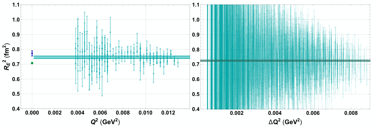
To illustrate the workings of this method, let us consider Fig. 3, where we plot the elements for the two datasets, as a function of . The blue and red bands provide the two corresponding bounds obtained by fitting a horizontal line using the NonlinearModelFit routine of Mathematica Inc. 2018. The corresponding values are given in the “Normalization-free” column of Table 1.
Note that the error on is decreasing with the increase of , and hence the obtained bounds are driven by the higher interval. In fact, one can apply a cut on the lowest values, without affecting the result.
Of course, this method only works if all the data points of a given dataset have the same normalization factor. In reality, the experiment of Bernauer et al. Bernauer et al. 2014 has a complicated normalization procedure, involving 31 normalization factors, and one can manage to obtain significant shifts of the data points by a different fit of these factors Higinbotham 2018, Higinbotham and McClellan 2019. These shifts could then be considered as a systematic normalization uncertainty which is only partially attributed to an overall normalization.
Nonetheless, one can identify subsets where the difference in normalization is overall. In the experimental data of Bernauer et al. these are, for example, normalization sets (see Supplement in Bernauer et al. 2014):
- 1.
3 (spectrometer A, MeV beam energy),
- 2.
1:3 (spectrometer B, MeV beam energy),
- 3.
6:9 (spectrometer B, MeV beam energy).
We have applied the method to each of this subsets separately (for GeV2) and obtained the same results (within statistical errors). The most precise result is the one from the 1:3 subset, because it is the largest in this region. The results for this dataset are shown in Fig. 4 and the second row of Table 1. The latter value is indeed a normalization-free bound.
We obtained the same results with the two datasets of Higinbotham Higinbotham 2018, generated from the data of Bernauer et al. Bernauer et al. 2014, and corresponding to significantly different radii. A subset of 106 data points in the very low- region ( GeV2) differs in an overall factor between the two datasets. Applying our method to this subset leads to the lower-bound value of fm, for both datasets, in exact agreement with our normalization-free result for the subset 1:3. We hence conclude that our method leads to a robust and accurate determination of the lower bound on from the form-factor data, even when they are prone to normalization uncertainties.
The lower bound resulting from the Bernauer dataset [ fm at 95% confidence level (CL)] is very accurate, although we emphasize that the error is only statistical. It can be compared with the recent proton-radius extractions in Fig. 1. It is somewhat in conflict with the H values Pohl et al. 2010, Antognini et al. 2013, and the Garching measurement of the transition frequency in H Beyer et al. 2017.
5 Conclusion
An extraction of the proton charge radius from scattering requires an extrapolation to zero momentum transfer, which nowadays is entangled in the analysis of data. We aim here to leave the extrapolation issues out of the interpretation of data. We show that the scattering may directly provide a lower bound on the proton charge radius, cf. Eq. (10) with Eq. (6). Thus, the lower bound is a directly observable quantity (to the extent that the form factor is), and is a more rigorous experimental outcome than the charge radius itself.
We have attempted a first determination of the lower bound on the proton charge radius from the available data in the region of below 0.02 GeV2. Our results for the two presently available experiments are given in Table 1. The last column therein shows the lower-bound values with the overall-normalization uncertainty being canceled out.
The lower bound, fm (95% CL), resulting from our “normalization-free” analysis of the data of Bernauer et al. Bernauer et al. 2014, rules out the shaded area in Fig. 1. The figure also shows the results of recent proton-radius determinations. In particular, this bound is in disagreement with the muonic-hydrogen values (green dots). We emphasize that the present determination of the lower bound does not involve any fitting of the -dependence with subsequent extrapolation to . On the other hand, the present analysis does not account for systematic errors in the experimental data, except for those that contribute to the overall normalization.
As the lower-bound function, defined in Eq. (6), is monotonically increasing with decreasing , the most stringent bound will be obtained from the lower range, provided that the accuracy does not deteriorate with decreasing . Therefore, with the forthcoming results of the PRad experiment Gasparian for the PRad at JLab Collaboration 2014, Peng and Gao 2016, one hopes to obtain a much better determination of the lower bound. The PRad data will reach down to and include a simultaneous measurement of the Møller scattering. The latter will allow to further reduce the systematic uncertainties.
Acknowledgements
We are grateful to Jan Bernauer, Michael Distler, Miha Mihovilović, and Thomas Walcher for sharing their data with us and helpful communications; to Douglas Higinbotham for checking some of our results and an interesting discussion; to Patricia Bickert, Ashot Gasparyan, Vadim Lensky, and Stefan Scherer for useful remarks on the manuscript. This work was supported by the Swiss National Science Foundation and the Deutsche Forschungsgemeinschaft (DFG) through the Collaborative Research Center 1044 [The Low-Energy Frontier of the Standard Model].
References
- Hofstadter and McAllister [1955] R. Hofstadter, R. W. McAllister, Electron scattering from the proton, Phys. Rev. 98 (1955) 217–218.
- Hofstadter [1957] R. Hofstadter, Nuclear and nucleon scattering of high-energy electrons, Ann. Rev. Nucl. Part. Sci. 7 (1957) 231–316.
- Bernauer et al. [2010] J. Bernauer, et al., High-Precision determination of the electric and magnetic form factors of the proton, Phys. Rev. Lett. 105 (2010) 242001.
- Bernauer et al. [2014] J. C. Bernauer, M. O. Distler, J. Friedrich, T. Walcher, Electric and magnetic form factors of the proton, Phys. Rev. C 90 (2014) 015206.
- Pohl et al. [2010] R. Pohl, et al., The size of the proton, Nature 466 (2010) 213–216.
- Antognini et al. [2013] A. Antognini, et al., Proton structure from the measurement of 2S-2P transition frequencies of muonic hydrogen, Science 339 (2013) 417–420.
- Mohr et al. [2012] P. J. Mohr, B. N. Taylor, D. B. Newell, Codata recommended values of the fundamental physical constants: 2010, Rev. Mod. Phys. 84 (2012) 1527–1605.
- Mohr et al. [2016] P. J. Mohr, D. B. Newell, B. N. Taylor, CODATA recommended values of the fundamental physical constants: 2014, Rev. Mod. Phys. 88 (2016) 035009.
- Beyer et al. [2017] A. Beyer, L. Maisenbacher, A. Matveev, R. Pohl, K. Khabarova, A. Grinin, T. Lamour, D. C. Yost, T. W. Hänsch, N. Kolachevsky, T. Udem, The rydberg constant and proton size from atomic hydrogen, Science 358 (2017) 79–85.
- Fleurbaey et al. [2018] H. Fleurbaey, S. Galtier, S. Thomas, M. Bonnaud, L. Julien, F. Biraben, F. Nez, M. Abgrall, J. Guna, New Measurement of the Transition Frequency of Hydrogen: Contribution to the Proton Charge Radius Puzzle, Phys. Rev. Lett. 120 (2018) 183001.
- Borisyuk [2010] D. Borisyuk, Proton charge and magnetic rms radii from the elastic scattering data, Nucl. Phys. A 843 (2010) 59–67.
- Hill and Paz [2010] R. J. Hill, G. Paz, Model independent extraction of the proton charge radius from electron scattering, Phys. Rev. D 82 (2010) 113005.
- Zhan et al. [2011] X. Zhan, K. Allada, D. Armstrong, J. Arrington, et al., High Precision Measurement of the Proton Elastic Form Factor Ratio at low , Phys. Lett. B 705 (2011) 59–64.
- Sick [2012] I. Sick, Problems with proton radii, Prog. Part. Nucl. Phys. 67 (2012) 473–478.
- Graczyk and Juszczak [2014] K. M. Graczyk, C. Juszczak, Proton radius from Bayesian inference, Phys. Rev. C 90 (2014) 054334.
- Arrington and Sick [2015] J. Arrington, I. Sick, Evaluation of the proton charge radius from e-p scattering, J. Phys. Chem. Ref. Data 44 (2015) 031204.
- Griffioen et al. [2016] K. Griffioen, C. Carlson, S. Maddox, Consistency of electron scattering data with a small proton radius, Phys. Rev. C 93 (2016) 065207.
- Lee et al. [2015] G. Lee, J. R. Arrington, R. J. Hill, Extraction of the proton radius from electron-proton scattering data, Phys. Rev. D 92 (2015) 013013.
- Higinbotham et al. [2016] D. W. Higinbotham, A. A. Kabir, V. Lin, D. Meekins, B. Norum, B. Sawatzky, Proton radius from electron scattering data, Phys. Rev. C 93 (2016) 055207.
- Horbatsch et al. [2017] M. Horbatsch, E. A. Hessels, A. Pineda, Proton radius from electron-proton scattering and chiral perturbation theory, Phys. Rev. C 95 (2017) 035203.
- Adamuscin et al. [2012] C. Adamuscin, S. Dubnicka, A. Dubnickova, New value of the proton charge root mean square radius, Prog. Part. Nucl. Phys. 67 (2012) 479–485.
- Lorenz et al. [2012] I. T. Lorenz, H. W. Hammer, U.-G. Meissner, The size of the proton - closing in on the radius puzzle, Eur. Phys. J. A 48 (2012) 151.
- Lorenz et al. [2015] I. Lorenz, U. Meißner, H. Hammer, Y. Dong, Theoretical constraints and systematic effects in the determination of the proton form factors, Phys. Rev. D 91 (2015) 014023.
- Alarcón et al. [2018] J. M. Alarcón, D. Higinbotham, C. Weiss, Z. Ye, Proton charge radius extraction from electron scattering data using dispersively improved chiral effective field theory, hep-ph/1809.06373 (2018).
- Bernauer [2016] J. C. Bernauer, Avoiding common pitfalls and misconceptions in extractions of the proton radius, nucl-th/1606.02159 (2016).
- Hayward and Griffioen [2018] T. B. Hayward, K. A. Griffioen, Evaluation of low- fits to and elastic scattering data, nucl-ex/1804.09150 (2018).
- Yan et al. [2018] X. Yan, D. W. Higinbotham, D. Dutta, H. Gao, A. Gasparian, M. A. Khandaker, N. Liyanage, E. Pasyuk, C. Peng, W. Xiong, Robust extraction of the proton charge radius from electron-proton scattering data, Phys. Rev. C 98 (2018) 025204.
- Perdrisat et al. [2007] C. F. Perdrisat, V. Punjabi, M. Vanderhaeghen, Nucleon Electromagnetic Form Factors, Prog. Part. Nucl. Phys. 59 (2007) 694–764.
- Hoferichter et al. [2016] M. Hoferichter, B. Kubis, J. Ruiz de Elvira, H. W. Hammer, U. G. Meißner, On the continuum in the nucleon form factors and the proton radius puzzle, Eur. Phys. J. A 52 (2016) 331.
- Mihovilović et al. [2017] M. Mihovilović, et al., First measurement of proton’s charge form factor at very low with initial state radiation, Phys. Lett. B 771 (2017) 194–198.
- Miller [2010] G. A. Miller, Transverse Charge Densities, Ann. Rev. Nucl. Part. Sci. 60 (2010) 1–25.
- Bracewell [2000] R. N. Bracewell, The Fourier transform and its applications, McGraw-Hill International Editions, 2000.
- Higinbotham [2018] D. W. Higinbotham, private communication (2018).
- Higinbotham and McClellan [2019] D. W. Higinbotham, R. E. McClellan, How Variation in Analytic Choices Can Affect Normalization Parameters and Proton Radius Extractions From Electron Scattering Data, physics.data-an/1902.08185 (2019).
- Distler et al. [2011] M. O. Distler, J. C. Bernauer, T. Walcher, The RMS Charge Radius of the Proton and Zemach Moments, Phys. Lett. B 696 (2011) 343–347.
- Inc. [2018] W. R. Inc., Mathematica, Version 11.3, 2018. Champaign, IL.
- Gasparian for the PRad at JLab Collaboration [2014] A. Gasparian for the PRad at JLab Collaboration, The PRad experiment and the proton radius puzzle, EPJ Web Conf. 73 (2014) 07006.
- Peng and Gao [2016] C. Peng, H. Gao, Proton Charge Radius (PRad) Experiment at Jefferson Lab, EPJ Web Conf. 113 (2016) 03007.