Stages of dynamics in the Fermi-Pasta-Ulam system as probed by the first Toda integral
Abstract
We investigate the long term evolution of trajectories in the Fermi-Pasta-Ulam (FPU) system, using as a probe the first non–trivial integral in the hierarchy of integrals of the corresponding Toda lattice model. To this end we perform simulations of FPU–trajectories for various classes of initial conditions produced by the excitation of isolated modes, packets, as well as ‘generic’ (random) initial data. For initial conditions corresponding to localized energy excitations, exhibits variations yielding ‘sigmoid’ curves similar to observables used in literature, e.g. the ‘spectral entropy’ or various types of ‘correlation functions’. However, is free of fluctuations inherent in such observables, hence it constitutes an ideal observable for probing the timescales involved in the stages of FPU dynamics. We observe two fundamental timescales: i) the ‘time of stability’ (in which, roughly, FPU trajectories behave like Toda), and ii) the ‘time to equilibrium’ (beyond which energy equipartition is reached). Below a specific energy crossover, both times are found to scale exponentially as an inverse power of the specific energy. However, this crossover goes to zero with increasing the degrees of freedom as , with . For ‘generic data’ initial conditions, instead, allows to quantify the continuous in time slow diffusion of the FPU trajectories in a direction transverse to the Toda tori.
1 Introduction
The numerical experiment of Fermi, Pasta and Ulam [20, 18] in 1954 aimed to probe ergodicity in an one–dimensional chain of weakly nonlinearly coupled oscillators. The discovery of FPU recurrences led to a substantial open question in Statistical Mechanics: Does a system with degrees of freedom, stemming from a generic perturbation to an integrable model, always tend to an ergodic state as becomes large? Several numerical studies confirm ergodicity in the FPU problem for large , and for various special types of initial conditions [4, 30, 31]. Nevertheless, despite a vast effort we are still far from reaching a rigorous answer to the above question. One obstruction to rigorous results stems from difficulties in implementing perturbation theory in the ‘thermodynamic limit’, i.e. when the energy per oscillator (specific energy) is small and fixed while becomes large.
Detailed reviews on the FPU problem can be found in [2, 27]. We quote here some important numerical and theoretical main lines of approach to the FPU problem, which are related to our present study:
i) Departure from the harmonic limit: the lowest order integrable approximation to the FPU is the chain of uncoupled oscillators constituting its linear normal modes. Initial conditions ‘à la Fermi’, i.e., low–frequency normal mode excitations, have been studied extensively [1, 3, 4, 21, 22, 23, 28, 36, 37, 38]. They are well known to lead to exponentially localized energy profiles in the space of normal modes. Such profiles persist for very long times (‘metastable states’), but eventually evolve to states closer to energy equipartition (‘equilibrium states’). In the harmonic limit (small specific energies) this behavior can be interpreted through the stability properties of particular low-dimensional invariant objects of the FPU phase space. Most notably, the ‘–breathers’ are Lyapunov periodic orbits forming the continuation of the linear modes [21, 22, 34]. On the other hand, the ‘–tori’ correspond to the extension, in the nonlinear regime, of quasi-periodic motions pertinent to excitations of packets of normal modes in the linear regime [12, 13, 14]. As far as the –breathers or –tori are stable (e.g. with respect to transverse perturbations), the metastability phenomenon can be understood as a case of ‘stickiness’ around these objects. From this viewpoint, however, it remains puzzling that the metastability phenomenon persists for specific energies higher than the stability thresholds of –breathers or –tori [21, 22, 12, 14], and clearly beyond the harmonic regime (although of course still small, i.e. ). One should note here that slow in time deviation from a quasi-integrable behavior seems to occur also in cases of more general types of initial conditions, where, from the beginning, the energy is distributed in the whole spectrum, instead of isolated packets of modes. In this case, we can compute the evolution of the autocorrelation functions for suitably defined phase space quantities [7, 8, 9, 10]. The equilibrium state is identified as the point of complete decay of the autocorrelation coefficients.
ii) Stochasticity threshold: In 1959 Chirikov published his celebrated works [15, 16, 26] on the existence of a stochasticity threshold in terms of specific energy in the FPU, which separates chaotic from weakly chaotic or regular motions. Chirikov’s threshold is derived by computing conditions under which the FPU resonances exhibit substantial overlapping. He finds that vanishes with like . In [40], Shepelyansky extended Chirikov’s results by including the case of low–mode excitations. Thus, the general conclusion from such studies is that one should expect stochasticity to prevail, and metastability phenomena to disappear, in the thermodynamic limit. Similar conclusions are reached when considering the dependence of the stability thresholds on for the –breathers [21, 22] and a weaker decay of the form for the –tori [14].
However, as noted in [40], any approach based on general criteria of resonance overlap cannot exclude the possibility that the system under investigation is very close to an integrable one, in which case estimates on resonances do not apply. In the words of Shepelyansky: ‘This point is very crucial for the –FPU problem, since at low energy it is very close to the Toda lattice. Due to that generally we should expect that, in contrast to the above estimates and numerical data the dynamics of the –FPU problem will be integrable’. In recent years, there has been increasing attention to Toda as a reference integrable model close to the FPU [5, 6, 14, 25, 37]. Already in 1982 the pioneering work of Ferguson et al. [19] put forward the idea that the higher polynomial order contact between FPU and Toda allows to associate the FPU’s integrable–like behavior (e.g. FPU recurrences) with Toda. In fact, this can be regarded as a ‘discrete’ analogue of the Zabusky–Kruskal approach, which associates the FPU with a different integrable continuous limit, i.e., the Korteweg–de Vries (KdV) equation [32].
In the present paper, we propose a simple method to measure the proximity of (evolving) FPU states, generated by various types of initial conditions, to the dynamics of the nearby integrable Toda model: this is to observe directly the evolution of the functions yielding the Toda integrals, for a single or an ensemble of FPU trajectories. An independent work along the same direction appeared recently in [25]. In the sequel, we focus on the evolution of only the first non-trivial Toda integral (besides the energy), denoted hereafter as . One has a constant value for any trajectory under the exact Toda dynamics, while varies along the FPU trajectories. As shown below, these variations allow to characterize the FPU stages of dynamics according to their proximity to the Toda dynamics. In particular, one can clearly identify ‘stickiness’ effects, and measure the times up to which the FPU trajectories remain sticky to nearby Toda tori.
Examples of this behavior, along with a corresponding quantitative analysis, are given in cases covering most widespread categories of initial conditions encountered in FPU literature. These roughly cover three classes of initial conditions: i) single mode or packet of modes excitations with coherent or random phases, ii) random data, where the whole energy spectrum has comparable power from the start, and iii) generic data close to energy equipartition. Cases (i) and (ii) are characterized by distinct phases of evolution of the FPU trajectories, which roughly correspond to the stages of dynamics recognized in [1, 37, 5]. We show below how allows to measure the timescales related with the stages of dynamics as well as the latter’s dependence on the system’s specific energy and number of degrees of freedom. In case (iii), using we provide direct evidence of diffusion taking place as the FPU trajectories wander in phase space transversally to ‘Toda tori’. This is useful also in interpreting the observed decay of the autocorrelation for the Toda integrals as reported in [5].
The paper is organized as follows: Section 2 deals with definitions and examples related to the utility of as an observable for featuring FPU–evolution. Section 3 analyses the information obtained by in numerical experiments covering each of the aforementioned class of initial conditions. Section 4 contains the basic conclusions of the present study.
2 The first Toda integral as an FPU–observable


Fermi, Pasta and Ulam [20] considered the one–dimensional lattice consisting of weakly nonlinearly coupled oscillators. The dynamics of this model is described by the Hamiltonian:
| (1) |
where is the –th particle’s displacement with respect to equilibrium and its canonically conjugate momentum. Fixed boundary conditions are imposed for .
The normal modes of the harmonic limit are defined by the canonical transformation . The normal mode energies are with frequencies , .
The FPU Hamiltonian has a third–order polynomial contact with the integrable Toda Hamiltonian [41]
| (2) |
where . Taylor–expanding the exponential , one obtains , where are the relative displacements.
The expressions of all the Toda integrals are given in [24, 29]. Besides , the first non–trivial Toda integral after adding and dividing with some constants, takes the form:
| (3) |
where fixed boundary conditions are imposed for , .
We outline the behavior of along FPU trajectories through the example of Fig.1. Consider the excitation of the first normal mode for the FPU system with , and particles. As will be described below, independently of the initial conditions considered, we find that, after sufficiently long integration, always tends to stabilize (apart from small fluctuations) to a final value, called hereafter, the ‘equilibrium value’ . In practice, is numerically computed by taking averages of in moving time windows long enough to absorb fluctuations. One notes that eventually the moving average stabilizes to a constant value after . For , only exhibits rapid and irregular fluctuations around the constant average . We argue below that this is an indication for a statistical equilibrium state reached by the system. The time is hereafter called the equilibrium time. The normalized is defined as:
| (4) |
In Fig.1 displays a sigmoidal evolution from 0 to 1. The detachment of from zero, which indicates an essential departure from quasi-integrable behavior, takes place at a time . During the time interval the behavior of for FPU and Toda is nearly indistinguishable. The time is hereafter called the time of stability. At longer times, tends sigmoidally towards the value 1, reached at time .
It is crucial to clarify in which sense reflects the time in which statistical equilibrium has been reached. We give numerical evidence in Fig.2, and we theoretically justify below, that the stabilization of to for is related to the following: (i) the variables , decorrelate (Fig.2(b),(f)), (ii) the energy spectrum reaches equipartition (Fig.2(d)).
Regarding (i), Fig.2(b) displays the evolution of the sums , for the same orbit as in Fig.1. Similar behavior is found for all orbits with initial conditions corresponding to localized excitations. For both sums oscillate, with maxima of the one sum corresponding to minima of the other. Between and , both sums tend sigmoidally to zero, while, beyond they become uncorrelated and both fluctuate irregularly around zero. Let us note, in respect, that a correlation sum similar to the above was considered by Parisi [33]
as an accurate and simple observable to be used in specifying the equilibrium time.
We will now show, that property (ii) above is connected with the correlation sums , both tending to zero for times beyond . To this end, for specific energies much smaller than unity, is well approximated by expanding the exponentials in (3) in Taylor series in powers of the quantities , . Up to quadratic terms we get (see Appendix A):
| (5) |
Due to Eq.(5), the near–constancy of for in Fig.2(a) emerges from the counterbalance of the sums and in Fig.2(b), which oscillate around a non–zero mean with nearly opposite phases. For , however, they both tend to zero. In fact, as shown in Appendix A, Eq.(5) can be recast as a sum over the energy spectrum :
| (6) |
This indicates that nearly corresponds to a linear combination of the energies , where more weight is given to the energies corresponding to low and high frequency modes, and less weight to modes in the middle of the spectrum (). Most notably, the sigmoid transition of from the value to is connected with the evolution of the energy spectrum from a localized one (for ) to near-equipartition for times . Since , one gets , implying that can also be interpreted as the ‘equipartition time’. On the other hand, the distribution of the momenta for approaches a Gaussian with dispersion (cf. Fig.2(e) and (f)). This is not far from the Gibbs measure for an equilibrium state with Hamiltonian (1). Thus, while energy equipartition alone does not necessarily imply an equilibrium state (see also numerical simulations below), in the above example energy equipartition is linked to and appears at the same timescale as the decorrelation between the phase space variables.

It is noteworthy that approximating formulas analogous to Eq.(6) can be derived relating all the Toda integrals with linear combinations of the spectral energies . Thus, a behavior analogous to the one found above for is expected to hold for all Toda integrals. This subject is currently under investigation.
Finally, we remark that the evolution of in Fig.1 is nearly indistinguishable from the evolution of the tail energy 11 1 A idea similar to the tail energy for generic packet excitations can be traced back to reference [35].
| (7) |
which has been proposed as an efficient observable for distinguishing stages of dynamics in the FPU problem (see [37, 4]). An additional method based on the times at which the FPU trajectories intersect an ‘equilibrium manifold’ [17] yields results similar to those of [37] found using the tail energy evolution. We find that the normalized Toda integral and the tail energy practically coincide for trajectories with initial low-mode excitations. However, as discussed below, is of use also in more generic initial conditions, in which the tail energy cannot be used.
3 Numerical Experiments
In this section we numerically investigate the stability, diffusion, and approach to equilibrium for FPU trajectories with various types of initial conditions, using as a probe the evolution of .


3.1 Classes of initial conditions and the evolution of J
We cluster different types of initial conditions into three main categories
referred to below as: (i) with ‘localized energy spectrum’, (ii) with
‘delocalized energy spectrum’, and (iii) ‘close to equipartition’.
(i) Localized energy spectrum: Case (i) contains FPU trajectories
with initial conditions corresponding to single–site excitations, and
packets of modes with coherent or random phases. The initial conditions
are controlled through the initial values assigned to the normal mode
variables , . To an initial energy
assigned to mode there corresponds a family of possible initial
conditions with ,
where and . A single–site
excitation is obtained by setting for all except one .
Here we consider the case . A ‘packet of modes’ excitation of
percentage corresponds to setting for all
in with and otherwise. In this
case, we can have initial phases ‘coherent’ (, here
), or ‘random’ (here is chosen from a uniform
distribution in ).
Figure 3(a) shows the evolution of along FPU trajectories with initial conditions corresponding to packets of various sizes (values of as denoted in the figure) and random phases, while the specific energy is kept fixed at . The packet (black) gives rise initially to a strongly localized energy spectrum which is nearly flat among the packet modes and develops an exponential tail for the rest of the modes, as shown in Fig.3(b). By progressively increasing the width of the packet (from to ), different localization patterns emerge in Fig.3(b). However, the evolution of in Fig.3(a) shows that equilibrium is reached at nearly equal times for all these trajectories. The dependence of both the ‘stability time’ and the equilibrium time on and is discussed in subsection 3.2.
(ii) Delocalized energy spectrum: case (ii) refers to non–equilibrium initial conditions with substantial power in the whole normal mode energy spectrum . As a basic example, we consider random initial positions and momenta extracted from a uniform distribution in the intervals , , with tuned numerically so that the total energy takes a selected value . Fig.4(a) shows the initial energy spectrum for such a choice of initial conditions, leading to specific energy . At the system appears as not being too far from energy equipartition, however, such initial conditions are not only far from the Gibbs measure but need longer equilibrium times than low–mode excitations. As shown in Fig.4(b) for a single realization, exhibits a similar sigmoidal evolution to the case (i). The approximations (5) and (6) yield curves nearly indistinguishable from the exact curve . Thus, the sigmoidal evolution is related to the slight redistribution of energies taking place as the system evolves to equilibrium. These are hard to distinguish using measures based directly on the spectrum , as for example, the spectral entropy ; see [38]). However measures with accuracy the time to equilibrium . Remarkably, for random initial positions and momenta turns to be of the same order as for the packet initial conditions, and actually somewhat larger than the times found for any ‘à la Fermi’ type of initial condition. This implies that stickiness to the Toda dynamics is a generic property not restricted to trajectories with localized initial energy spectrum.
(iii) Initial conditions close to equipartition: here we consider two subcases of initial conditions, namely far from or close to the Gibbs distribution . In the first subcase, we consider initial conditions called hereafter ‘random momenta’, in which we simply set , and randomly chosen from a uniform distribution in the interval , with . One obtains , and hence a spectrum with . As an alternative, we fix the normal mode variables , , with and randomly chosen with uniform distribution in the interval . Both these types of initial condition lead to spectra close to equipartition, but far from the distribution function associated with statistical equilibrium. Instead, in the second subcase, hereafter called ‘close to equilibrium’, as in the works [5, 6, 7, 8] we approximate a Gibbs distribution function for the normal mode variables by considering only the quadratic part of the Hamiltonian . The function becomes a Gaussian
| (8) |
Setting ensures the specific energy is equal to for any random realization in the above distribution.
One key feature of the numerical experiments with all the above initial conditions is that (for single trajectories, or averaged over trajectories with different realizations of the initial conditions) exhibits no systematic change of its value (e.g. of sigmoid form) allowing to define a timescale to equilibrium as in the case of the experiments in class (i) and (ii). Fig.5(a) and (b) shows two examples of the evolution of the average for ten realizations of trajectories with initial conditions belonging to the ‘random phase’ and ‘random momenta’ subclass. Despite the absence of sigmoid evolution, one may still argue that for initial conditions far from equilibrium, a certain time is required for these trajectories to drift substantially in phase space so as to approach a state of equilibrium. Such an approach cannot be detected by the evolution of the energy spectra , since the latter are set from the start close to energy equipartition. Nevertheless, the form of the curves in Fig.5 suggests the trajectories undergo diffusion in the direction normal to the integral surfaces defined by the Toda integrals, or at least the first one. Such diffusion can be detected by measuring the evolution of the dispersion in the values of over trajectories
| (9) |
where . Subtracting the initial value is necessary to absorb the spreading in the initial values of due to the random generator of initial conditions. Fig.6a Shows as a function of for a set of 30 trajectories with ‘random initial momenta’. The solid line has logarithmic slope equal to 1, indicating a normal diffusion law . Notice that the diffusion stops after a time . The spreading in the values of after this time has measure , indicating that the trajectories have spread over parts of the phase space covering the whole possible range of values of consistent with a fixed specific energy equal to .
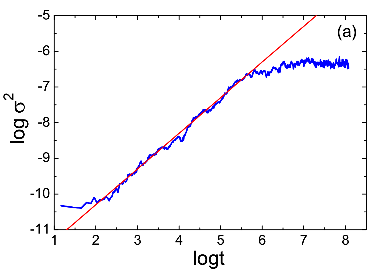

On the other hand, it is really remarkable that a similar spreading is found for initial conditions very close to the Gibbs measure, as exemplified in Fig.6(b). Now, the initial conditions are chosen by the distribution function of Eq.(8), thus they represent a state as close as possible to statistical equilibrium already at the starting point of the simulation. Yet, we observe that the underlying integrable dynamics of the associated Toda model leaves its traces in this case too, since the trajectories diffuse transversally to the integral surface of the integral with a very slow speed, comparable to the one in initial conditions far from equilibrium. Measuring this speed at various energy levels, as well as for different Toda integrals represents a challenging numerical task, since it requires many trajectory realizations per parameter set considered in order to ensure a good statistics (setting in the above experiments is marginal in this respect). Instead, the speed of approach to equilibrium is measured more easily via the sigmoid curves in experiments of classes (i) and (ii), a computation to which we now turn our attention.
3.2 Intensive quantities and a single timescale


We first investigate for which types of initial conditions the behavior of and associated timescales (of ‘stability’ or ’approach to equilibrium’, see section 2) exhibit a dependence on . It turns out that only random initial data lead to –independent results. For example, Fig.7(a) shows the sigmoid curves when considering the excitation of the first normal mode (case (i)), with ranging from 512 to 8192. The curves are distinguished, in particular as regards the ‘stability’ times characterized by the onset of the rising part of the sigmoid evolution, even if the equilibrium times are similar for all . In comparison, Fig.7(b) shows the same computation but for initial conditions extracted by random positions and momenta (case (ii)). Superposing the sigmoid curves for various shows a near-coincidence at all times.
We note that a similar behavior to Fig.7(b) holds for initial data as those of Fig.3. Thus, packet excitations with random phases exhibit –independence in the timescales associated with the evolution of . This is in agreement with the results first reported in [3], where the authors aim to unify ‘incompatible’ earlier findings in the FPU literature (see [3] and references therein) on the dependence of various scaling laws on the energy , when exciting packets of modes with coherent phases, or the specific energy , when the initial phases are random. It is also in agreement with the work [14], where it is found that extensive packets with coherent phases give rise to exponentially localized energy spectra of the form , with , , i.e., depending on rather than .
Exploiting the property of –independence, we can characterize the timescales involved in the evolution of for classes of trajectories based on some form of random initial data. Computing allows to obtain a good estimate of the ‘stability time’, from the size of the initial plateau of the corresponding sigmoid curve, and the time of approach to equilibrium, when the second plateau is reached. Due to the numerical indications for –independence one may reasonably argue that the results hold in the thermodynamic limit ( keeping constant). Focusing, as an example, on trajectories with random initial positions and momenta, the sigmoid curves for the normalized Toda integral are reproduced in Fig.7(c). With an appropriate time–shift (inset), those curves fall one onto the other as shown in Fig.7(d). We typically find beyond a crossover specific energy (see below) for some depending on the type of initial conditions. Since the shift in the sigmoid curves takes place in a logarithmic time axis, the above facts imply that allows to characterize the scalings with of both the initial ‘stability time’ and the ‘time to equilibrium’. One has
with . At practical level, the possibility to extrapolate scaling laws from the ‘stability’ to the ‘approach to equilibrium’ phase allows to translate results found for to analogous results for , even when is much larger than and hence hard to compute by direct numerical experiments. One has to compute in respect the initial part of the curve , up to the detachment from the first plateau. We also note that the numerical complexity for computing is , which is much better than the complexity of any computation requiring knowledge of the evolution of the energy spectra .


All the above results hold asymptotically for sufficiently large. Instead, for small we may find deviations from the law which are –dependent. In particular, we find transient exponential laws , up to a crossover specific energy . However, we can make use of ’s asymptotic independence in order to locate the specific energy crossover . The numerical procedure is the following: the sigmoid curves or (as in Fig.7(d)) serve as exemplary curves which determine the power-law dependence on of the timescales and . These curves are –independent for random–based initial conditions. Starting with small system sizes and by lowering the energy, one eventually encounters the crossover: the law describing these timescales changes from power to exponential and a dependence on emerges. Practically, this means that for the –curves do not match with their exemplary counterparts, as in the example of Fig.8.
Two sets of three sigmoid curves are shown in Fig.8(a) (experiments with random initial positions and momenta) for decreasing energies with constant logarithmic step, namely , , and (black set) or (green set). Only the initial parts of the –curves are shown, up to the value . At the curves for the two values of nearly coincide, while a mismatch appears at , clearly becoming larger by further lowering the energy. Fig.8(b) explains this mismatching in terms of the stability time , defined as the times when the curve first crosses the value . Inspecting Fig.8(b), the delineation of to the –independent final power-law (dashed line, obtained by fitting the data for ) occurs at smaller crossover specific energies as increases. Repeating the study for the initial excitation of a packet of modes with random phases (Fig.8(c) and (d)) find the same trend of with , with slightly different exponents. Notice that, for energies smaller than the crossover, one cannot always safely distinguish between an exponential law or a power law with steeper exponent than the exponent of the –independent profile. For example, in Fig.8(d) the case could be fairly well fitted by a steeper power-law, in accordance with the interpretation via the ‘six-wave resonant interactions’ in [39]. Leaving open such questions, we here emphasize the utility of observing for answering them, as well as for characterizing the asymptotic regime, which indicates that as : the latter fact suffices to exclude exponentially-long lasting deviations from the equilibrium state at the thermodynamic limit ( Fig.8(e)).


Finally, we examine how the scaling laws on equilibrium times are affected by particular choices of initial conditions. To this end we consider six different types of initial conditions for the FPU system with and , exciting: (1) the first normal mode, (2) the lowermost frequency packet of modes with zero initial phases (as in [12, 13, 14]), (3) the lowermost–frequency packet of modes with random initial phases (as in [3]), (4) random initial momenta, (5) random initial positions and finally, (6) random initial positions/momenta. The corresponding sigmoid curves are displayed in Fig.9(a), with solid lines for and dashed lines for ( in all cases). We immediately note the –dependence of the behavior of the sigmoid curves for (1) and (2). Also, in (4) the spectrum exhibits equipartition already at , hence . On the other hand, in (5) and (6) starts below , since the energy spectrum somewhat favors high modes (see Eq.(6)). Finally, all curves equilibrate at , i.e. very close to , as predicted by Eq.(6) for all equal.
Using now the numerical procedure described above, we calculate the equilibrium times for five out of the six types of initial conditions in Fig.9(a) and for (we exclude (4) in which ). As Fig.9(b) shows, in all cases we find , with the exponent varying between 2.5 (for the low–frequency mode excitations), to 3 (random positions and/or momenta). To within numerical uncertainties, one is tempted to conclude that yielding, in the initial data, more power to the high-frequency part of the mode spectrum results in steeper laws , i.e., trajectories more stable against the approach to equilibrium. We leave open the question of the associated scalings when only high modes are excited, a case not largely considered so far in literature.
4 Conclusion
We examined the role of the first Toda integral as an indicator of the evolution, and crossing of various ‘stages of dynamics’ for FPU trajectories. This is accomplished by computing the time variations of the ‘normalized’ Toda integral (section 2) when an FPU trajectory is substituted within . Our main conclusions are summarized below.
Despite its apparent simplicity, proves to be a very efficient indicator allowing to clearly distinguish stages of FPU dynamics for a wide class of initial conditions. In particular, it allows to clearly define two times, called the ‘time of stability’ , and the ‘time to equilibrium’ . For times the FPU trajectories remain extremely close to the original integral surface . Thus, can be interpreted as a time of stickiness to the original Toda integral surface. On the other hand, marks the approach of the system to equilibrium.
For classes of initial conditions based on random initial data (in position or momenta, or the phases for normal mode variables), as long as the initial energy spectrum is not in equipartition, the times and are connected via a ‘sigmoid’ evolution of the curves . For large , the graph of becomes –independent, so that we obtain one representative sigmoid curve described by one time-scale with exponents , depending on the class of initial conditions considered. However, by lowering we cross to an energy regime where the system becomes –depended and its corresponding time-scales extend exponentially like , . Such a phenomenon seems to disappear in the thermodynamic limit for two cases of random initial data with non-equipartitioned energy spectra.
We finally examine the information drawn from computing time fluctuations of in cases in which the system is initially at energy equipartition, with the initial conditions being distributed either far or close to the Gibbs measure. In such cases, through we can clearly compute a speed of diffusion transversally to the Toda integral surfaces. This speed is always small, implying that an underlying nearly-integrable dynamics holds even when the initial conditions are close to equipartition, and even close to the final equilibrium state.
As a final comment, we expect similar features, as those encountered for the evolution of the first Toda integral, to appear also for the other Toda integrals, a subject currently under investigation. In fact, treating such integrals analogously as in Eq.(6) allows to conjecture that, at low energies, this behavior will be reflected satisfactorily by their harmonic approximations. A detailed investigation of this subject is proposed for future study.
5 Acknowledgments
We are indebted to G. Benettin and A. Ponno for very fruitful discussions which significantly improved the present work. H.C. was supported by the State Scholarship Foundation (IKY) operational Program: ‘Education and Lifelong Learning–Supporting Postdoctoral Researchers’ 2014-2020, and is co–financed by the European Union and Greek national funds.
Appendix A Analytic estimates
The quadratic terms of (3) derive from the terms and . immediately yields the terms and yields the terms after Taylor–expanding any of the terms etc.
Now summing all quadratic terms together,
| (10) |
their expression easily simplifies by matching terms like which can be replaced by . Furthermore, it is and which approximates the quadratic terms in (10) and gives the expression (4):
.
Under the Fourier transform the above expression takes the form (5). In particular, it is and , where and the off–diagonal sum is approximately zero. Therefore, we get that
References
- [1] Bambusi D and Ponno A (2006) On Metastability in FPU. Comm. Math. Phys 264: 539.
- [2] Berman GP, Izrailev FM (2005) The Fermi-Pasta-Ulam problem: 50 years of progress. Chaos 15: 015104.
- [3] Benettin G, Livi R and Ponno A. (2009) The Fermi-Pasta-Ulam Problem: Scaling Laws vs. Initial Conditions. J Stat Phys 135: 873-893.
- [4] Benettin G and Ponno A. (2011) Time–Scales to Equipartition in the Fermi-Pasta-Ulam Problem: Finite-Size Effects and Thermodynamic Limit. J Stat Phys 144: 793.
- [5] Benettin G, Christodoulidi H and Ponno A (2013) The Fermi-Pasta-Ulam problem and its underlying integrable dynamics. J Stat Phys 152(2): 195-212.
- [6] Benettin G, Pasquali S. and Ponno A (2018) The Fermi-Pasta-Ulam problem and its underlying integrable dynamics. J Stat Phys 171(4): 521–542.
- [7] Carati A, Galgani L, Giorgilli A and Paleari S (2007) Fermi-Pasta-Ulam phenomenon for generic initial data. Phys Rev E 76: 022104.
- [8] Carati A and Galgani L (1999) Journal of Statistical Physics 94: 859-869.
- [9] Carati A, Maiocchi A, Galgani L and Amati G (2015) The Fermi-Pasta-Ulam System as a Model for Glasses. Math Phys Anal Geom 18: 31.
- [10] Carati A and Ponno A (2018) Chopping Time of the FPU –Model J Stat Phys 170(5): 883-894.
- [11] L. Casetti, M. Cerruti-Sola, M. Pettini, and E. G. D. Cohen, Phys. Rev. E 55, 6566 (1997).
- [12] Christodoulidi H, Efthymiopoulos C and Bountis T (2010) Energy localization on q-tori, long-term stability, and the interpretation of Fermi-Pasta-Ulam recurrences Phys Rev E 81: 016210/1-16.
- [13] Christodoulidi H and C. Efthymiopoulos (2013) Low-dimensional q-Tori in FPU Lattices: Dynamics and Localization Properties. Physica D 261: 92-113.
- [14] Christodoulidi H (2017) Extensive packet excitations in FPU and Toda lattices. EPL 119: 40005.
- [15] Chirikov BV (1959) Resonance processes in magnetic traps. At Energ 6: 630 (1960 Engl. Transl., J. Nucl. Energy Part C: Plasma Phys. 1 253)
- [16] Chirikov BV (1979) A universal instability of many-dimensional oscillator systems. Phys Rep 52: 263-379.
- [17] Danieli C, Campbell DK and Flach S (2017) Intermittent many-body dynamics at equilibrium. Phys Rev E 95, 060202(R).
- [18] Dauxois T (2008) Fermi, Pasta, Ulam, and a mysterious lady. Physics Today 61(1): 55-57.
- [19] Ferguson W E Jr, Flaschka H and McLaughlin D W (1982) Nonlinear normal modes for the Toda Chain. J Comp Phys 45: 157-209.
- [20] Fermi E, Pasta J and Ulam S (1995) Studies of non linear problems. Los Alamos report No LA-1940.
- [21] Flach S, Ivanchenko MV and Kanakov OI (2005) q-Breathers and the Fermi-Pasta-Ulam Problem. Phys Rev Lett 95: 064102.
- [22] Flach S, Ivanchenko MV and Kanakov OI (2006) q-Breathers in Fermi-Pasta-Ulam chains: Existence, localization, and stability. Phys Rev E 73: 036618.
- [23] Flach S and Ponno A (2008) The Fermi-Pasta-Ulam problem Periodic orbits, normal forms and resonance overlap criteria. Physica D 237: 908-917.
- [24] Flaschka H (1974) The Toda lattice. II. Existence of integrals. Phys Rev B 9(4): 1924-1925.
- [25] Goldfriend T and Kurchan T, Equilibration of Quasi-Integrable Systems. https://arxiv.org/abs/1810.06121
- [26] Izrailev FM and Chirikov BV (1966) Statistical properties of a nonlinear string. Dokl Akad Nauk SSSR 166(1): 57-59
- [27] Gallavotti G (ed.) The Fermi-Pasta-Ulam Problem: A Status Report. Lect. Notes Phys., vol. 728. Springer, Berlin-Heidelberg (2008)
- [28] Genta T, Giorgilli A, Paleari S and Penati T (2012) Packets of resonant modes in the Fermi-Pasta-Ulam system. Phys Lett A 376: 2038-2044.
- [29] Hénon M (1974) Integrals of the Toda lattice. Phys Rev B 9: 1921-1923.
- [30] Kantz H, Livi R and Ruffo S (1994) Equipartition thresholds in chains of anharmonic oscillators. J Stat Phys 76: 627.
- [31] Kantz H (1989) Vanishing stability thresholds in the thermodynamic limit of nonintegrable conservative systems. Physica D 39(2-3): 322-335.
- [32] Kruskal MD and Zabusky NJ (1965) Interaction of Solitons in a Collisionless Plasma and the Recurrence of Initial States. Phys Rev Lett 15: 240.
- [33] Parisi G (1997) On the approach to equilibrium of a Hamiltonian chain of anharmonic oscillators. EPL 40(4):357–362.
- [34] Penati T and Flach S (2007) Tail resonances of Fermi-Pasta-Ulam q-breathers and their impact on the pathway to equipartition. Chaos 17: 023102/1-16.
- [35] Paleari S and Penati T (2005) Equipartition times in a Fermi-Pasta-Ulam system. Discrete Contin Dyn Syst: 710–719.
- [36] Ponno A, Bambusi D (2005) Korteweg-de Vries equation and energy sharing in Fermi-Pasta-Ulam. Chaos 15: 015107.
- [37] Ponno A, Christodoulidi H, Skokos Ch and Flach S (2011) The two-stage dynamics in the Fermi-Pasta-Ulam problem: from regular to diffusive behavior. Chaos 21(4): 043127.
- [38] Livi R, Pettini M, Ruffo S, Sparpaglione M and Vulpiani A (1985) Equipartition threshold in nonlinear large Hamiltonian systems The Fermi-Pasta-Ulam model. Phys Rev A 31: 1039–1045.
- [39] Lvov YV and Onorato M (2018) Double Scaling in the Relaxation Time in the -Fermi-Pasta-Ulam-Tsingou Model. Phys Rev Lett 120: 144301.
- [40] Shepelyansky DL (1997) Low-energy chaos in the Fermi-Pasta-Ulam problem. Nonlinearity 10(5): 1331.
- [41] Toda M (1970) Waves in Nonlinear Lattice. Prog Theor Phys Suppl 45: 174-200.
*