跳到论文正文
W Papers独立论文阅读器 arXiv:1812.01320 论文正文 计算阅读时间 · 0%
引用这篇论文根据当前论文元数据生成,正式投稿前建议核对。


License: arXiv.org perpetual non-exclusive license
arXiv:1812.01320v1 [econ.TH] 04 Dec 2018
Abstract.

This paper studies the income fluctuation problem with capital income risk (i.e., dispersion in the rate of return to wealth). Wealth returns and labor earnings are allowed to be serially correlated and mutually dependent. Rewards can be bounded or unbounded. Under rather general conditions, we develop a set of new results on the existence and uniqueness of solutions, stochastic stability of the model economy, as well as efficient computation of the ergodic wealth distribution. A variety of applications are discussed. Quantitative analysis shows that both stochastic volatility and mean persistence in wealth returns have nontrivial impact on wealth inequality.

Keywords: Income fluctuation, optimality, stochastic stability, wealth distribution.

The Income Fluctuation Problem with Capital Income Risk: Optimality and Stability11 1 We thank Jess Benhabib, Christopher Carroll, Fedor Iskhakov, Larry Liu, Ronald Stauber and Chung Tran for valuable feedback and suggestions, as well as audience members at the RSE seminar at the Australian National University in 2017.
Email addresses: qingyin.ma@anu.edu.au,   john.stachurski@anu.edu.au,   atoda@ucsd.edu.

Qingyin Maa,   John Stachurskib   and   Alexis Akira Todac

a, bResearch School of Economics, The Australian National University

cDepartment of Economics, University of California, San Diego

November 15, 2018

1. Introduction

The income fluctuation problem refers to the broad class of decision problems that characterize the optimal consumption-saving behavior for agents facing stochastic income streams. In most cases, agents are subject to idiosyncratic shocks and borrowing constraints. Markets are incomplete so idiosyncratic risks cannot be fully diversified or hedged. The model represents one of the fundamental workhorses of modern macroeconomics, and has been adopted to study a large variety of important topics, ranging from asset pricing, life-cycle choice, fiscal policy, social security, to income and wealth inequality, among many others. See, for example, Schechtman 1976, Deaton and Laroque 1992, Huggett 1993, Aiyagari 1994, Carroll 1997, Chamberlain and Wilson 2000, Cagetti and De Nardi 2008, De Nardi et al. 2010, Guner et al. 2011, Guvenen 2011, Meghir and Pistaferri 2011, Meyer and Sullivan 2013, Guvenen and Smith 2014 and Heathcote et al. 2014.

In recent years, researchers have come to investigate an important mechanism in the income fluctuation framework—the dispersion in rates of return to wealth, referred to below as the capital income risk. Early studies are provided by Angeletos and Calvet 2005 and Angeletos 2007. These works highlight that the macroeconomic effects of idiosyncratic capital income risk can be both qualitatively distinct from those of idiosyncratic labor income risk and quantitatively significant.

An especially important set of applications concerns wealth inequality. As is well known in the literature, the classic income fluctuation frameworks of Huggett 1993 and Aiyagari 1994, in which returns to wealth are homogeneous across agents, fail to reproduce the high inequality and the fat upper tail of wealth distributions in many economies. Such empirical failure has prompted researchers to investigate models with uninsured capital income risk. Entrepreneurial risk, a representative example of capital income risk, is studied by Quadrini 2000 and Cagetti and De Nardi 2006. By introducing heterogeneity across agents in their work and entrepreneurial ability, these studies successfully generate skewed wealth distributions that are more similar to those observed in the U.S. data.

Moreover, in an OLG economy with intergenerational transmission of wealth, Benhabib et al. 2011 show that capital income risk is the driving force of the heavy-tail properties of the stationary wealth distribution. In a Blanchard-Yaari style economy, Benhabib et al. 2016 show that idiosyncratic investment risk has a big impact on generating a double Pareto stationary wealth distribution. In another important contribution, Gabaix et al. 2016 point out that a positive correlation of returns with wealth (“scale dependence”) in addition to persistent heterogeneity in returns (“type dependence”) can well explain the speed of changes in the tail inequality observed in the data. An important work that is highly pertinent to the present paper is Benhabib et al. 2015. In a stylized infinite horizon income fluctuation problem with capital income risk, the authors prove that there exists a unique stationary wealth distribution that displays fat tail.

On the empirical side, using twelve years of population data from Norway’s administrative tax records, Fagereng et al. 2016a; Fagereng et al. 2016b document that individuals earn markedly different average returns to both their financial assets (a standard deviation of 14%14\%) and net worth (a standard deviation of 8%8\%). Wealth returns are heterogeneous both within and across asset classes. Returns are positively correlated with the wealth level and highly persistent over time. In addition, wealth returns are (mildly) correlated across generations.

Although theoretical, empirical and quantitative studies all reveal the significant economic impact of capital income risk, existing models of capital income risk in the income fluctuation framework are highly stylized. For example, the assumptions of iid labor income process, iid wealth return process and their mutual independence made by Benhabib et al. 2015 are rejected by the empirical data in several economies (see, e.g., Kaplan and Violante 2010, Guvenen and Smith 2010 and Fagereng et al. 2016a; Fagereng et al. 2016b). As Benhabib et al. 2015 point out, adding positive correlations in labor earnings and wealth returns enriches model dynamics in that it captures economic environments with limited social mobility.

To our best knowledge, a general theory of capital income risk in the income fluctuation framework has been missing in the literature. This raises concerns about whether or not existing views on the economic impact of capital income risk hold in general, as well as whether or not modeling capital income risk in more generic and realistic settings is technically achievable. To be specific, several important questions are:

  • •

    Do correlations in the wealth return process (e.g., those caused by mean persistence or stochastic volatility of wealth returns) enhance or dampen the macroeconomic impact of capital income risk?

  • •

    What if, in addition to serial correlation, the wealth return process and the labor earnings process are mutually correlated?

  • •

    Does an optimal policy always exist in these generalized settings? If it does, is it unique?

  • •

    Does the stochastic law of motion for optimal wealth accumulation yield a stationary distribution of wealth?

  • •

    If it does, is the model economy globally stable, in the sense that the stationary distribution is unique and can be approached by the distributional path from any starting point?

  • •

    How do we compute the optimal policy and the stationary wealth distribution in practice?

These questions are highly significant, in the sense that a negative answer to any of them will pose a threat to the existing findings concerning capital income risk. However, due to technical limitations, these questions have not been investigated in a general income fluctuation framework. In this paper, we attempt to fill this gap. To this end, we extend the standard income fluctuation problem by characterizing the following essential features.

  • •

    Agents face idiosyncratic rate of return to wealth {Rt}\{R_{t}\} (capital income risk) and idiosyncratic labor earnings {Yt}\{Y_{t}\} (labor income risk), both of which are affected by a generic, exogenous Markov process {zt}\{z_{t}\}.

  • •

    Supports of {Rt}\{R_{t}\} and {Yt}\{Y_{t}\} are bounded or unbounded, and, in either case, allowed to contain zero.

  • •

    The reward (utility) function is bounded or unbounded, and no specific structure is imposed beyond differentiability, concavity and the usual slope conditions.

As can be seen, general {Rt}\{R_{t}\} and {Yt}\{Y_{t}\} processes that are serially correlated and mutually dependent are covered by our framework. Moreover, consumption can become either arbitrarily small or arbitrarily large, so that agents are allowed to borrow up to the highest sustainable level of debt, creating rich and substantial model dynamics reflecting agents’ borrowing activity.22 2 See the discussion of Rabault 2002.

We make several tightly connected contributions on optimality, stochastic stability and computation of this generalized income fluctuation problem.

First, we prove that the Coleman operator adapted to this framework is indeed an “nn-step” contraction mapping in a complete metric space of candidate consumption policies, even when rewards are unbounded. The unique fixed point is shown to be the optimal policy (also unique in the candidate space), and several important properties (e.g., continuity and monotonicity) are derived. To tackle unboundedness, we draw on and extend Li and Stachurski 2014 by adding capital income risk and constructing a metric that evaluates consumption differences in terms of marginal utility. To obtain contractions under a minimal level of restriction, we focus our key assumption on bounding the long-run growth rate of wealth returns.

We show that this assumption is indeed equivalent to bounding the spectral radius of an expected wealth return operator (a bounded linear operator) by 1/β1/\beta. As a result, it is similar to the assumptions made by recent literature regarding the operator theoretic method, which have been proven both necessary and sufficient for the existence and uniqueness of solutions in a variety of models (see, e.g., Hansen and Scheinkman 2009; Hansen and Scheinkman 2012, Borovička and Stachurski 2017 and Toda 2018). Our assumption is easy to verify numerically. For example, when the state space for the exogenous Markov process {zt}\{z_{t}\} is finite, verifying this assumption is as convenient as finding the largest modulus of the set of eigenvalues for a given matrix.

Second, as our most significant contribution, we show that the model economy is globally stable, even in the presence of capital income risk. Specifically, there exists a unique stationary distribution for the state process (including wealth and the exogenous Markov state), and, given any initial state, the distributional path of the state process generated via optimal consumption and wealth accumulation converges to the stationary distribution as time iterates forward. The idea of proof goes as follows. Based on the optimality results established in the previous step, existence of a stationary distribution is guaranteed under some further restrictions on agents’ level of patience, plus some mild assumptions on the stochastic properties of the exogenous state and the labor income processes. The key is to show that the wealth process is bounded in probability.

The proof of global stability is more tricky and separated into two scenarios.

(Scenario I) When the exogenous state process {zt}\{z_{t}\} is independent and identically distributed, so are {Rt}\{R_{t}\} and {Yt}\{Y_{t}\}, and wealth is the only state variable remaining. We show that, with some additional concavity structure imposed, the model economy is monotone, allowing us to use some new results in the field of stochastic stability (due to Kamihigashi and Stachurski 2014; Kamihigashi and Stachurski 2016). Based on these results, both global stability and the Law of Large Numbers are established. In this case, convergence of the distributional path to its stationarity is in the form of weak convergence. Moreover, the added concavity assumption holds for standard utilities such as CRRA or the logarithm utility. Notably, even in the current case, our theory extends the stability theory of Benhabib et al. 2015, since we allow {Rt}\{R_{t}\} and {Yt}\{Y_{t}\} to be dependent on each other (a more detailed comparison is given below).

(Scenario II) When the exogenous state process {zt}\{z_{t}\} is Markovian, {Rt}\{R_{t}\} and {Yt}\{Y_{t}\} are in general autocorrelated and mutually dependent, and the structure of monotone economy is lost due to the added exogenous state. As a result, the order theoretic approach used in the previous case is no longer applicable. In response to that, we aim to exploit the traditional theory of stochastic stability (see, e.g., Meyn and Tweedie 2009). Specifically, we provide sufficient conditions for the state process to be ψ\psi-irreducible, strongly aperiodic and a positive Harris chain, which in turn guarantee global stability and the Law of Large Numbers. Convergence here is in total variation norm distance, which is stronger than weak convergence. Our sufficient conditions are easy to verify in applications, and centered around existence of density representations for the exogenous state process and the labor earnings process. We only require that supports of the two densities contain respectively a nontrivial compact subset and a certain “small” interval. Importantly, no further concavity structure is required.

Moreover, we show in this scenario that if we add the same concavity structure as we do in scenario I and some other mild assumptions (e.g., existence of densities for the wealth return process and geometric drift property of the labor earnings process), then the model economy is indeed VV-geometrically ergodic. As a result, convergence to the stationary distribution occurs at a geometric speed.

Since an iid process is a special Markov process, as a byproduct, the theory in scenario II serves as an alternative stability theory when the exogenous state process is iid. As can be seen from the discussion above, neither of the two theories is “stronger” than the other in this circumstance. On the one hand, global stability in scenario I is established under an additional concavity assumption, which is not required for global stability in scenario II. On the other hand, we make no assumptions on the density structure of the key stochastic processes in scenario I as we do in scenario II.

Based on the established stability and ergodicity results, the unique stationary distribution can be approximated via tracking a single state process simulated according to the optimal consumption and wealth accumulation rules, which is highly efficient. The real caveat is that, in presence of capital income risk, there can be very large realized values of wealth (and consumption), causing serious problems to numerical computation of the optimal policy. However, this problem is alleviated in our setting. We show that, under our maintained assumptions, the optimal policy is concave and asymptotically linear with respect to the wealth level. Hence, at large levels of wealth, the optimal consumption rule can be well approximated via linear extrapolation.

We provide several important applications. First, we illustrate how our theory can be applied to modeling capital income risk in different scenarios. Then, we provide a numerical example in which we explore the quantitative effect of stochastic volatility and mean persistence of the wealth return process on wealth inequality. In the calibrated economy, our quantitative analysis shows that both these two factors lead to lower tail exponents of the stationary wealth distribution and higher Gini coefficients, and thus a higher level of wealth inequality.

In terms of connections to the existing literature, the most closely related results are those found in the recent paper Benhabib et al. 2015. Like us, the authors study capital income risk in an income fluctuation framework. On the one hand, their paper proves an important theoretical result—the stationary wealth distribution has a fat tail, a topic not treated by the present paper (tail properties are only studied by us numerically).

On the other hand, our theory of optimality and stochastic stability is considerably sharper and covers a much broader range of applications. Specifically, to avoid technical complication, Benhabib et al. 2015 assume that {Rt}\{R_{t}\} and {Yt}\{Y_{t}\} are iid, mutually independent, supported on bounded closed intervals with strictly positive lower bounds, and that their distributions are represented by densities. Albeit helpful for simplifying analysis and deriving tail properties, these assumptions rule out important features observed in the real economy (e.g., mean persistence and stochastic volatility in the empirical labor earnings and wealth return processes, as discussed). Moreover, the strictly positive lower bound for {Yt}\{Y_{t}\} prevents agents from borrowing up to the highest sustainable level of debt, hiding substantial model dynamics.33 3 As discussed in Rabault 2002, in this case, agents are guaranteed a strictly positive minimum level of consumption, so the marginal value of consumption is bounded, and the problem can be easily solved by constructing supremum norm contractions. However, relaxing this assumption allows agents to systematically avoid exhausting their borrowing capacity. As described above, all these assumptions are relaxed in our framework.

Regarding earlier literature, specific types of capital income risk are modeled by Quadrini 2000, Angeletos and Calvet 2005, Cagetti and De Nardi 2006 and Angeletos 2007 in general equilibrium frameworks. In comparison, the present paper focuses on constructing a “more general” one-sector framework and deriving sharper theoretical results, which, of course, could potentially benefit “more general” general equilibrium analysis.

Moreover, since we tackle unbounded rewards and the associated technical complication, our paper is also related to Rabault 2002, Carroll 2004, Kuhn 2013 and Li and Stachurski 2014. These works develop different methods to handle the issue of unboundedness in standard income fluctuation problems (ones without capital income risk). While Carroll 2004 constructs a weighted supremum norm contraction and works with the Bellman operator, the other three works focus on the Coleman operator. In particular, Rabault 2002 exploits the monotonicity structure, Kuhn 2013 applies a version of the Tarski’s fixed point theorem, while Li and Stachurski 2014 constructs a contraction mapping based on a metric that evaluates consumption differences in marginal values. As discussed above, the present paper draws on and extends Li and Stachurski 2014 by incorporating capital income risk.

The rest of this paper is structured as follows. Section 2 formulates the problem. Section 3 establishes optimality results. Sufficient conditions for the existence and uniqueness of optimal policies are discussed. Section 4 focuses on stochastic stability. Global stability and some further properties are studied. Section 5 provides a set of applications. All proofs are deferred to the appendix.

2. Set up

This section sets up the income fluctuation problem to be studied. As a first step, we introduce some mathematical techniques and notation used in this paper.

2.1. Preliminaries

Let ℕ\mathbbm{N}, ℝ\mathbbm{R} and ℝ+\mathbbm{R}_{+} be the natural, real and nonnegative real numbers respectively. Given topological space 𝖲\mathsf{S}, let ℬ⁡(𝖲)\mathscr{B}(\mathsf{S}) be the Borel σ\sigma-algebra and let 𝒫⁡(𝖲)\mathscr{P}(\mathsf{S}) be the set of probability measures on ℬ⁡(𝖲)\mathscr{B}(\mathsf{S}). A stochastic kernel QQ on 𝖲\mathsf{S} is a map Q:𝖲×ℬ⁡(𝖲)→[0,1]Q\colon\mathsf{S}\times\mathscr{B}(\mathsf{S})\to[0,1] such that

  • •

    x↦Q⁡(x,B)x\mapsto Q(x,B) is ℬ⁡(𝖲)\mathscr{B}(\mathsf{S})-measurable for each B∈ℬ⁡(𝖲)B\in\mathscr{B}(\mathsf{S}) and

  • •

    B↦Q⁡(x,B)B\mapsto Q(x,B) is a probability measure on ℬ⁡(𝖲)\mathscr{B}(\mathsf{S}) for each x∈𝖲x\in\mathsf{S}.

Let b​c​𝖲bc\mathsf{S} be the set of bounded continuous functions on 𝖲\mathsf{S}. A stochastic kernel QQ is called Feller if x↦∫h⁡(y)​Q​(x,⁡𝑑y)x\mapsto\int h(y)Q(x,\mathop{}\!\mathrm{d}y) is in b​c​𝖲bc\mathsf{S} whenever h∈b​c​𝖲h\in bc\mathsf{S}.

For all t∈ℕt\in\mathbbm{N}, we define the tt-th order kernel as

Q1:=Q,Qt(x,B):=∫Qt−1(y,B)Q(x,dy)(x∈𝖲,B∈ℬ(𝖲)).Q^{1}:=Q,\quad Q^{t}(x,B):=\int Q^{t-1}(y,B)Q(x,\mathop{}\!\mathrm{d}y)\quad(x\in\mathsf{S},B\in\mathscr{B}(\mathsf{S})).

The value Qt​(x,B)Q^{t}(x,B) represents the probability of transitioning from xx to BB in tt steps. Furthermore, for all μ∈𝒫⁡(𝖲)\mu\in\mathscr{P}(\mathsf{S}), we define μ​Qt∈𝒫⁡(𝖲)\mu Q^{t}\in\mathscr{P}(\mathsf{S}) as

(μ​Qt)​(B):=∫Qt​(x,B)​μ​(⁡𝑑x)(B∈ℬ⁡(𝖲)).(\mu Q^{t})(B):=\int Q^{t}(x,B)\mu(\mathop{}\!\mathrm{d}x)\qquad(B\in\mathscr{B}(\mathsf{S})).

A sequence {μn}⊂𝒫⁡(𝖲)\{\mu_{n}\}\subset\mathscr{P}(\mathsf{S}) is called tight, if, for all ε>0\varepsilon>0, there exists a compact K⊂𝖲K\subset\mathsf{S} such that μn​(𝖲\K)≤ε\mu_{n}(\mathsf{S}\backslash K)\leq\varepsilon for all nn. We say that μn\mu_{n} converges to μ\mu weakly and write μn→μ\mu_{n}\mathrel{{\mathop{\rightarrow}\limits}}\mu if μ∈𝒫⁡(𝖲)\mu\in\mathscr{P}(\mathsf{S}) and ∫h​⁡d​μn→∫h​⁡𝑑μ\int h\mathop{}\!\mathrm{d}\mu_{n}\rightarrow\int h\mathop{}\!\mathrm{d}\mu for all bounded continuous h:𝖲→ℝh\colon\mathsf{S}\rightarrow\mathbbm{R}.

A stochastic kernel QQ is called bounded in probability if the sequence {Qt​(x,⋅)}t≥0\{Q^{t}(x,\cdot)\}_{t\geq 0} is tight for all x∈𝖲x\in\mathsf{S}. We call ψ∈𝒫⁡(𝖲)\psi\in\mathscr{P}(\mathsf{S}) stationary for QQ if ψ​Q=ψ\psi Q=\psi. We say that QQ is globally stable if there exists a unique stationary distribution ψ\psi in 𝒫⁡(𝖲)\mathscr{P}(\mathsf{S}) and ψ0​Qt→ψ\psi_{0}Q^{t}\mathrel{{\mathop{\to}\limits}}\psi for all ψ0∈𝒫⁡(𝖲)\psi_{0}\in\mathscr{P}(\mathsf{S}).

Let KK be a bounded linear operator from b​c​𝖲bc\mathsf{S} to itself and ∥⋅∥\|\cdot\| be the supremum norm on b​c​𝖲bc\mathsf{S}. The operator norm and spectral radius of KK are defined by

∥K∥:=sup{∥Kg∥:g∈bc𝖲,∥g∥≤1}andr(K):=limm→∞∥Km∥1/m.\|K\|:=\sup\{\|Kg\|:g\in bc\mathsf{S},\;\|g\|\leq 1\}\quad\text{and}\quad r(K):=\lim_{m\to\infty}\|K^{m}\|^{1/m}.

In particular, when 𝖲\mathsf{S} is finite, KK becomes a square matrix, and the spectral radius r⁡(K)r(K) reduces to maxλ⁡|λ|\max_{\lambda}|\lambda|, where λ\lambda ranges over the set of eigenvalues of KK. (See, e.g., page 663 of Aliprantis and Border 2006).

In what follows, (Ω,ℱ,ℙ)(\Omega,\mathscr{F},\mathbbm{P}) is a fixed probability space on which all random variables are defined, while 𝔼\mathbbm{E}\, is expectations with respect to ℙ\mathbbm{P}.

2.2. The income fluctuation problem

We introduce capital income risk and consider a generalized income fluctuation problem as follows

max⁡𝔼⁡{∑t≥0βt​u​(ct)}\displaystyle\max\,\mathbbm{E}\,\left\{\sum_{t\geq 0}\beta^{t}u(c_{t})\right\}
(1) s.t. at+1=Rt+1​(at−ct)+Yt+1,\displaystyle a_{t+1}=R_{t+1}(a_{t}-c_{t})+Y_{t+1},
0≤ct≤at,(a0,z0)=(a,z)​ given,\displaystyle 0\leq\;c_{t}\leq a_{t},\quad(a_{0},z_{0})=(a,z)\text{ given},

where β∈[0,1)\beta\in[0,1) is a state-independent discount factor, uu is the utility function, the control process {ct}t≥0\{c_{t}\}_{t\geq 0} is consumption, {Rt}t≥1\{R_{t}\}_{t\geq 1} is a gross rate of return on wealth and {Yt}t≥1\{Y_{t}\}_{t\geq 1} is labor income. The return and income processes obey

Rt\displaystyle R_{t} =R⁡(zt,ζt),{ζt}t≥1∼ν,\displaystyle=R\left(z_{t},\zeta_{t}\right),\quad\left\{\zeta_{t}\right\}_{t\geq 1}\mathrel{{\mathop{\sim}\limits}}\nu,
(2) Yt\displaystyle Y_{t} =Y⁡(zt,ηt),{ηt}t≥1∼μ,\displaystyle=Y\left(z_{t},\eta_{t}\right),\quad\left\{\eta_{t}\right\}_{t\geq 1}\mathrel{{\mathop{\sim}\limits}}\mu,

where RR and YY are nonnegative real-valued measurable functions, {ζt}\{\zeta_{t}\} and {ηt}\{\eta_{t}\} are innovations, and {zt}t≥0\{z_{t}\}_{t\geq 0} is a time-homogeneous 𝖹\mathsf{Z}-valued Markov process with Feller stochastic kernel PP, where 𝖹\mathsf{Z} is a Borel subset of ℝm\mathbbm{R}^{m} paired with the usual relative topology.

Throughout we make the following assumption on the agent’s utility.

Assumption 2.1.

The utility function u:ℝ+→{−∞}∪ℝu\colon\mathbbm{R}_{+}\rightarrow\{-\infty\}\cup\mathbbm{R} is twice differentiable on (0,∞)(0,\infty) and satisfies

  1. (1)

    u′>0u^{\prime}>0 and u′′<0u^{\prime\prime}<0 everywhere on (0,∞)(0,\infty), and

  2. (2)

    u′​(c)→∞u^{\prime}(c)\rightarrow\infty as c→0c\rightarrow 0 and u′​(c)→0u^{\prime}(c)\rightarrow 0 as c→∞c\rightarrow\infty.

Example 2.1.

A typical example that meets assumption 2.1 is the CRRA utility

(3) u⁡(c)=c1−γ/(1−γ)if ​γ>0,γ≠1andu⁡(c)=log⁡cif ​γ=1,u(c)=c^{1-\gamma}/(1-\gamma)\quad\text{if }\gamma>0,\,\gamma\neq 1\quad\text{and}\quad u(c)=\log c\quad\text{if }\gamma=1,

where γ>0\gamma>0 is the coefficient of relative risk aversion.

2.3. Further notation

We use xx and x^\hat{x} to denote respectively the current and next period random variables. In addition,

(4) 𝔼a,z:=𝔼[⋅|(a0,z0)=(a,z)]and𝔼z:=𝔼[⋅|z0=z].\mathbbm{E}\,_{a,z}:=\mathbbm{E}\,\left[\,\cdot\,\big|\,(a_{0},z_{0})=(a,z)\right]\quad\text{and}\quad\mathbbm{E}\,_{z}:=\mathbbm{E}\,\left[\,\cdot\,\big|\,z_{0}=z\right].

In particular, for any integrable function ff,

(5) 𝔼z​f​(z^,R^,Y^)=∫f⁡[z^,R⁡(z^,ζ^),Y⁡(z^,η^)]​P​(z,⁡𝑑z^)​ν​(⁡𝑑ζ^)​μ​(⁡𝑑η^).\mathbbm{E}\,_{z}\,f(\hat{z},\hat{R},\hat{Y})=\int f\left[\hat{z},R(\hat{z},\hat{\zeta}),Y\left(\hat{z},\hat{\eta}\right)\right]P(z,\mathop{}\!\mathrm{d}\hat{z})\nu(\mathop{}\!\mathrm{d}\hat{\zeta})\mu(\mathop{}\!\mathrm{d}\hat{\eta}).

3. Optimality Results

In this section, we show that, with bounded or unbounded rewards, the Coleman operator adapted to the income fluctuation problem above is an nn-step contraction mapping on a complete metric space of candidate policies, and that the unique fixed point is the optimal policy. To that end, we make the following assumptions.

Assumption 3.1.

There exists n∈ℕn\in\mathbbm{N} such that θ:=βnsupz∈𝖹𝔼zR1⋯Rn<1\theta:=\beta^{n}\sup_{z\in\mathsf{Z}}\mathbbm{E}\,_{z}R_{1}\cdots R_{n}<1.

Assumption 3.2.

For all z∈𝖹z\in\mathsf{Z}, we have ∑t=1∞βt​𝔼z​Yt<∞\sum_{t=1}^{\infty}\beta^{t}\mathbbm{E}\,_{z}Y_{t}<\infty.

Assumption 3.3.

supz∈𝖹𝔼z​R^<∞\sup_{z\in\mathsf{Z}}\mathbbm{E}\,_{z}\,\hat{R}<\infty,   supz∈𝖹𝔼z​u′​(Y^)<∞\sup_{z\in\mathsf{Z}}\mathbbm{E}\,_{z}u^{\prime}(\hat{Y})<\infty and supz∈𝖹𝔼z​R^​u′​(Y^)<∞\sup_{z\in\mathsf{Z}}\mathbbm{E}\,_{z}\hat{R}u^{\prime}(\hat{Y})<\infty.

Assumption 3.4.

The functions z↦R⁡(z,ζ)z\mapsto R(z,\zeta), z↦Y⁡(z,η)z\mapsto Y(z,\eta), z↦𝔼z​R^z\mapsto\mathbbm{E}\,_{z}\hat{R} and z↦𝔼z​R^​u′​(Y^)z\mapsto\mathbbm{E}\,_{z}\hat{R}\,u^{\prime}(\hat{Y}) are continuous.

Example 3.1.

For all bounded continuous function ff on 𝖹\mathsf{Z}, define

K​f​(z):=𝔼z​R^​f​(z^),z∈𝖹.Kf(z):=\mathbbm{E}\,_{z}\hat{R}f(\hat{z}),\quad z\in\mathsf{Z}.

Then KK is a bounded linear operator by assumption 3.3. Let r⁡(K)r(K) be the spectral radius of KK. Then assumption 3.1 holds if and only if β​r​(K)<1\beta r(K)<1. We prove this result in the appendix.

Example 3.2.

Let {zt}\{z_{t}\} be a finite-state Markov chain on 𝖹:={i1,⋯,iN}\mathsf{Z}:=\{i_{1},\cdots,i_{N}\} with transition matrix Π\Pi (a “discrete” stochastic kernel). Let diag​(⋅)\text{diag}(\cdot) denote the diagonal matrix generated by elements in the bracket, and, with slight abuse of notation, let

𝔼​R​(z,ζ):=∫R⁡(z,ζ)​ν​(⁡𝑑ζ)andD:=diag​(𝔼​R​(i1,ζ),⋯,𝔼​R​(iN,ζ)).\mathbbm{E}\,R(z,\zeta):=\int R(z,\zeta)\nu(\mathop{}\!\mathrm{d}\zeta)\quad\text{and}\quad D:=\text{diag}\left(\mathbbm{E}\,R(i_{1},\zeta),\cdots,\mathbbm{E}\,R(i_{N},\zeta)\right).

In this case, the operator KK in example 3.1 reduces to the matrix K=Π​DK=\Pi D. Therefore, assumption 3.1 holds if and only if r⁡(Π​D)<1/βr(\Pi D)<1/\beta. In particular, r⁡(Π​D)r(\Pi D) equals the largest modulus of all the eigenvalues of Π​D\Pi D.

Example 3.3.

Based on the Hölder’s inequality, to show assumption 3.3, it suffices to find some p,q∈[1,∞]p,q\in[1,\infty] such that 1/p+1/q=11/p+1/q=1 and

supz∈𝖹𝔼z​R^p<∞andsupz∈𝖹𝔼z​u′​(Y^)q<∞.\sup_{z\in\mathsf{Z}}\mathbbm{E}\,_{z}\,\hat{R}^{p}<\infty\quad\text{and}\quad\sup_{z\in\mathsf{Z}}\mathbbm{E}\,_{z}u^{\prime}(\hat{Y})^{q}<\infty.

To establish the required results, we (temporarily) assume a0>0a_{0}>0 and set the asset space as (0,∞)(0,\infty). The state space for the state process {(at,zt)}t≥0\{(a_{t},z_{t})\}_{t\geq 0} is then44 4 Note that the second condition of assumption 2.1 and assumption 3.3 imply that ℙ{Yt>0}=1\mathbbm{P}\{Y_{t}>0\}=1 for all t≥1t\geq 1 (although YtY_{t} is allowed to be arbitrarilly close to zero). Hence, ℙ{at>0}=1\mathbbm{P}\{a_{t}>0\}=1 for all t≥1t\geq 1 by the law of motion (2.2). It thus makes no difference to optimality to exclude zero from the asset space. Doing this simplifies analysis since uu and u′u^{\prime} are finite away from zero. It actually allows us to propose a useful metric and apply the contraction approach, as to be shown later.

𝖲0:=(0,∞)×𝖹∋(a,z).\mathsf{S}_{0}:=(0,\infty)\times\mathsf{Z}\ni(a,z).

Consider the maximal asset path {a~t}\{\tilde{a}_{t}\} defined by

(6) a~t+1=Rt+1​a~t+Yt+1and(a~0,z~0)=(a,z)​given.\tilde{a}_{t+1}=R_{t+1}\,\tilde{a}_{t}+Y_{t+1}\quad\text{and}\quad(\tilde{a}_{0},\tilde{z}_{0})=(a,z)\;\text{given}.
Lemma 3.1.

If assumptions 3.1–3.2 hold, then ∑t≥0βt​𝔼a,z​a~t\sum_{t\geq 0}\beta^{t}\mathbbm{E}\,_{a,z}\,\tilde{a}_{t} is finite for all (a,z)∈𝖲0(a,z)\in\mathsf{S}_{0}.

A feasible policy is a Borel measurable function c:𝖲0→ℝc\colon\mathsf{S}_{0}\rightarrow\mathbbm{R} with 0≤c⁡(a,z)≤a0\leq c(a,z)\leq a for all (a,z)∈𝖲0(a,z)\in\mathsf{S}_{0}. Given any feasible policy cc and initial condition (a,z)∈𝖲0(a,z)\in\mathsf{S}_{0}, the asset path generated by (c,(a,z))(c,(a,z)) is the sequence {at}t≥0\{a_{t}\}_{t\geq 0} in (2.2) when ct=c⁡(at,zt)c_{t}=c(a_{t},z_{t}) and (a0,z0)=(a,z)(a_{0},z_{0})=(a,z). The lifetime value of any feasible policy cc is the function Vc:𝖲0→{−∞}∪ℝV_{c}\colon\mathsf{S}_{0}\rightarrow\{-\infty\}\cup\mathbbm{R} defined by

Vc​(a,z)=𝔼a,z​{∑t≥0βt​u​[c⁡(at,zt)]},V_{c}(a,z)=\mathbbm{E}\,_{a,z}\left\{\sum_{t\geq 0}\beta^{t}u\left[c(a_{t},z_{t})\right]\right\},

where {at}\{a_{t}\} is the asset path generated by (c,(a,z))(c,(a,z)). Notice that Vc​(a,z)<∞V_{c}(a,z)<\infty for any feasible cc and any (a,z)∈𝖲0(a,z)\in\mathsf{S}_{0}. This is because, by assumption 2.1, there exists a constant LL such that u⁡(c)≤c+Lu(c)\leq c+L, and hence

Vc​(a,z)≤𝔼a,z​∑t≥0βt​u​(at)≤𝔼a,z​∑t≥0βt​u​(a~t)≤∑t≥0βt​𝔼a,z​a~t+L1−β.V_{c}(a,z)\leq\mathbbm{E}\,_{a,z}\sum_{t\geq 0}\beta^{t}u(a_{t})\leq\mathbbm{E}\,_{a,z}\sum_{t\geq 0}\beta^{t}u(\tilde{a}_{t})\leq\sum_{t\geq 0}\beta^{t}\mathbbm{E}\,_{a,z}\,\tilde{a}_{t}+\frac{L}{1-\beta}.

The last expression is finite by lemma 3.1.

A feasible policy c∗c^{*} is called optimal if Vc≤Vc∗V_{c}\leq V_{c^{*}} on 𝖲0\mathsf{S}_{0} for any feasible policy cc. In the present setting, the finiteness of VcV_{c} for each feasible policy, the strict concavity of uu, and the convexity of the set of feasible policies from each (a,z)∈𝖲0(a,z)\in\mathsf{S}_{0} imply that for each given parameterization, at most one optimal policy exists.

A feasible policy is said to satisfy the first order optimality conditions if

(7) (u′∘c)​(a,z)≥β​𝔼z​R^​(u′∘c)​(R^​[a−c⁡(a,z)]+Y^,z^)\left(u^{\prime}\circ c\right)(a,z)\geq\beta\,\mathbbm{E}\,_{z}\,\hat{R}\left(u^{\prime}\circ c\right)\left(\hat{R}\left[a-c(a,z)\right]+\hat{Y},\,\hat{z}\right)

for all (a,z)∈𝖲0(a,z)\in\mathsf{S}_{0}, and equality holds when c⁡(a,z)<ac(a,z)<a. Moreover, a feasible policy is said to satisfy the transversality condition if, for all (a,z)∈𝖲0(a,z)\in\mathsf{S}_{0},

(8) limt→∞βt​𝔼a,z​[(u′∘c)​(at,zt)​at]=0.\lim_{t\rightarrow\infty}\beta^{t}\mathbbm{E}\,_{a,z}\left[\left(u^{\prime}\circ c\right)(a_{t},z_{t})\,a_{t}\right]=0.
Theorem 3.1.

If assumptions 2.1 and 3.1–3.2 hold, and cc is a feasible policy that satisfies both the first order optimality conditions and the transversality condition, then cc is an optimal policy.

When does an optimal policy exist, and how can we compute it? To answer these questions, following Li and Stachurski 2014, we use a contraction argument, where the underlying function space is set to 𝒞\mathscr{C}, the functions c:𝖲0→ℝc\colon\mathsf{S}_{0}\rightarrow\mathbbm{R} such that

  1. (1)

    cc is continuous,

  2. (2)

    cc is increasing in the first argument,

  3. (3)

    0<c⁡(a,z)≤a0<c(a,z)\leq a for all (a,z)∈𝖲0(a,z)\in\mathsf{S}_{0}, and

  4. (4)

    sup(a,z)∈𝖲0|(u′∘c)​(a,z)−u′​(a)|<∞\sup_{(a,z)\in\mathsf{S}_{0}}\left|(u^{\prime}\circ c)(a,z)-u^{\prime}(a)\right|<\infty.

To compare two policies, we pair 𝒞\mathscr{C} with the distance

(9) ρ⁡(c,d):=‖u′∘c−u′∘d‖:=sup(a,z)∈𝖲0|(u′∘c)​(a,z)−(u′∘d)​(a,z)|\rho(c,d):=\left\|u^{\prime}\circ c-u^{\prime}\circ d\right\|:=\sup_{(a,z)\in\mathsf{S}_{0}}\left|\left(u^{\prime}\circ c\right)(a,z)-\left(u^{\prime}\circ d\right)(a,z)\right|

that evaluates the maximal difference in terms of marginal utility. Note that

(10) c∈𝒞⟹∃K∈ℝ+​ s.t. ​u′​(a)≤(u′∘c)​(a,z)≤u′​(a)+K,∀(a,z)∈𝖲0.c\in\mathscr{C}\Longrightarrow\exists K\in\mathbbm{R}_{+}\text{ s.t. }u^{\prime}(a)\leq(u^{\prime}\circ c)(a,z)\leq u^{\prime}(a)+K,\,\forall(a,z)\in\mathsf{S}_{0}.

Moreover, while elements of 𝒞\mathscr{C} are not generally bounded, one can show that ρ\rho is a valid metric on 𝒞\mathscr{C}. In particular, ρ\rho is finite on 𝒞\mathscr{C} since ρ⁡(c,d)≤‖u′∘c−u′‖+‖u′∘d−u′‖\rho(c,d)\leq\left\|u^{\prime}\circ c-u^{\prime}\right\|+\left\|u^{\prime}\circ d-u^{\prime}\right\|, and the last two terms are finite by the definition of 𝒞\mathscr{C}.

Proposition 3.1.

(𝒞,ρ)(\mathscr{C},\rho) is a complete metric space.

Proposition 3.2.

If assumptions 2.1 and 3.1–3.3 hold, c∈𝒞c\in\mathscr{C}, and, for all (a,z)∈𝖲0(a,z)\in\mathsf{S}_{0},

(11) (u′∘c)​(a,z)=max⁡{β​𝔼z​R^​(u′∘c)​(R^​[a−c⁡(a,z)]+Y^,z^),u′​(a)},\left(u^{\prime}\circ c\right)(a,z)=\max\left\{\beta\,\mathbbm{E}\,_{z}\,\hat{R}\left(u^{\prime}\circ c\right)\left(\hat{R}\left[a-c(a,z)\right]+\hat{Y},\,\hat{z}\right),u^{\prime}(a)\right\},

then cc satisfies both the first order optimality conditions and the transversality condition. In particular, cc is an optimal policy.

Inspired by proposition 3.2, we aim to characterize the optimal policy as the fixed point of the Coleman operator TT defined as follows: for fixed c∈𝒞c\in\mathscr{C} and (a,z)∈𝖲0(a,z)\in\mathsf{S}_{0}, the value of the image T​cTc at (a,z)(a,z) is defined as the ξ∈(0,a]\xi\in(0,a] that solves

(12) u′​(ξ)=ψc​(ξ,a,z),u^{\prime}(\xi)=\psi_{c}(\xi,a,z),

where ψc\psi_{c} is the function on

(13) G:={(ξ,a,z)∈ℝ+×(0,∞)×𝖹:0<ξ≤a}G:=\left\{(\xi,a,z)\in\mathbbm{R}_{+}\times(0,\infty)\times\mathsf{Z}\colon 0<\xi\leq a\right\}

defined by

(14) ψc​(ξ,a,z):=max⁡{β​𝔼z​R^​(u′∘c)​[R^​(a−ξ)+Y^,z^],u′​(a)}.\psi_{c}(\xi,a,z):=\max\left\{\beta\mathbbm{E}\,_{z}\hat{R}(u^{\prime}\circ c)[\hat{R}(a-\xi)+\hat{Y},\,\hat{z}],\,u^{\prime}(a)\right\}.

The following propositions show that the Coleman operator TT is a well-defined self-map from the candidate space (𝒞,ρ)(\mathscr{C},\rho) into itself.

Proposition 3.3.

If assumptions 2.1 and 3.1–3.3 hold, then for each c∈𝒞c\in\mathscr{C} and (a,z)∈𝖲0(a,z)\in\mathsf{S}_{0}, there exists a unique ξ∈(0,a]\xi\in(0,a] that solves (12).

Proposition 3.4.

If assumptions 2.1 and 3.1–3.4 hold, then T​c∈𝒞Tc\in\mathscr{C} for all c∈𝒞c\in\mathscr{C}.

Recall nn and θ\theta defined in assumption 3.1. We now provide our key optimality result.

Theorem 3.2.

If assumptions 2.1 and 3.1–3.4 hold, then TnT^{n} is a contraction mapping on (𝒞,ρ)(\mathscr{C},\rho) with modulus θ\theta. In particular,

  1. (1)

    TT has a unique fixed point c∗∈𝒞c^{*}\in\mathscr{C}.

  2. (2)

    The fixed point c∗c^{*} is the unique optimal policy in 𝒞\mathscr{C}.

  3. (3)

    For all c∈𝒞c\in\mathscr{C} and k∈ℕk\in\mathbbm{N}, we have ρ⁡(Tn​k​c,c∗)≤θk​ρ​(c,c∗)\rho(T^{nk}c,c^{*})\leq\theta^{k}\rho(c,c^{*}).

4. Stochastic Stability

This section focuses on stochastic stability of the generalized income fluctuation problem. We first provide sufficient conditions for the existence of a stationary distribution and then explore conditions for uniqueness and ergodicity.

Now we add zero back into the asset space, and consider a larger state space for the state process {(at,zt)}t≥0\{(a_{t},z_{t})\}_{t\geq 0}, denoted by

𝖲:=[0,∞)×𝖹∋(a,z).\mathsf{S}:=[0,\infty)\times\mathsf{Z}\ni(a,z).

We extend c∗c^{*} to 𝖲\mathsf{S} by setting c∗​(0,z)=0c^{*}(0,z)=0 for all z∈𝖹z\in\mathsf{Z}. Together, c∗c^{*} and the transition functions for {at}\{a_{t}\}, {Rt}\{R_{t}\} and {Yt}\{Y_{t}\} determine a Markov process with state vector st:=(at,zt)s_{t}:=(a_{t},z_{t}) taking values in the state space 𝖲\mathsf{S}. Let QQ denote the corresponding stochastic kernel. The law of motion of {st}\{s_{t}\} is

at+1\displaystyle a_{t+1} =R⁡(zt+1,ζt+1)​[at−c∗​(at,zt)]+Y⁡(zt+1,ηt+1),\displaystyle=R\left(z_{t+1},\zeta_{t+1}\right)\left[a_{t}-c^{*}\left(a_{t},z_{t}\right)\right]+Y\left(z_{t+1},\eta_{t+1}\right),
(15) zt+1\displaystyle z_{t+1} ∼P⁡(zt,⋅)\displaystyle\sim P\left(z_{t},\,\cdot\,\right)

4.1. Existence of a stationary distribution

To obtain existence of a stationary distribution, we make the following assumptions.

Assumption 4.1.

There exists α∈(0,1)\alpha\in(0,1) such that

  1. (1)

    β​𝔼z​R^​u′​[R^​(1−α)​a]≤u′​(a)\beta\,\mathbbm{E}\,_{z}\hat{R}\,u^{\prime}[\hat{R}\left(1-\alpha\right)a]\leq u^{\prime}(a) for all (a,z)∈𝖲0(a,z)\in\mathsf{S}_{0},55 5 Here we adopt the convention that 0⋅∞=00\cdot\infty=0 so that assumption 4.1 does not rule out the case ℙ⁡{Rt=0∣zt−1=z}>0\mathbbm{P}\{R_{t}=0\mid z_{t-1}=z\}>0. Indeed, as would be shown in proofs, all the conclusions of this paper still hold if we replace this condition by the weaker alternative: β​𝔼z​R^​u′​[R^​(1−α)​a+α​Y^]≤u′​(a)\beta\,\mathbbm{E}\,_{z}\hat{R}\,u^{\prime}[\hat{R}\left(1-\alpha\right)a+\alpha\hat{Y}]\leq u^{\prime}(a) for all (a,z)∈𝖲0(a,z)\in\mathsf{S}_{0}, while maintaining the second part of assumption 4.1. and

  2. (2)

    there exists n∈ℕn\in\mathbbm{N} such that (1−α)nsupz∈𝖹𝔼zR1⋯Rn<1(1-\alpha)^{n}\sup_{z\in\mathsf{Z}}\mathbbm{E}\,_{z}R_{1}\cdots R_{n}<1.

Assumption 4.2.

supt≥1𝔼z​Yt<∞\sup_{t\geq 1}\mathbbm{E}\,_{z}\,Y_{t}<\infty for all z∈𝖹z\in\mathsf{Z}.

Assumption 4.3.

The stochastic kernel PP is bounded in probability.

Example 4.1.

For homogeneous utility functions (e.g., CRRA), if the first condition of assumption 4.1 holds for some a∈(0,∞)a\in(0,\infty), then it must hold for all a∈(0,∞)a\in(0,\infty). To see this, let kk be the degree of homogeneity. Then we have

β​𝔼z​R^​u′​[R^​(1−α)​a]/u′​(a)=β​𝔼z​R^1+k​(1−α)kfor all ​a∈(0,∞).\beta\mathbbm{E}\,_{z}\hat{R}u^{\prime}[\hat{R}(1-\alpha)a]/u^{\prime}(a)=\beta\mathbbm{E}\,_{z}\hat{R}^{1+k}(1-\alpha)^{k}\quad\text{for all }a\in(0,\infty).

The right hand side is constant in aa.

Example 4.2.

Recall example 3.2, where {zt}\{z_{t}\} is a finite-state Markov chain. Consider the CRRA utility defined in (3). Define further the column vector

V:=(𝔼​R​(i1,ζ)1−γ,⋯,𝔼​R​(iN,ζ)1−γ)′.V:=\left(\mathbbm{E}\,R(i_{1},\zeta)^{1-\gamma},\cdots,\mathbbm{E}\,R(i_{N},\zeta)^{1-\gamma}\right)^{\prime}.

Then, assumption 4.1 holds whenever

(16) max{r(ΠD),1}<(β∥ΠV∥)−1/γ.\max\{r(\Pi D),1\}<\left(\beta\|\Pi V\|\right)^{-1/\gamma}.

To see this, the first condition of assumption 4.1 holds if there exists α∈(0,1)\alpha\in(0,1) such that (1−α)−γ​β​𝔼z​R^1−γ≤1(1-\alpha)^{-\gamma}\beta\mathbbm{E}\,_{z}\hat{R}^{1-\gamma}\leq 1 for all z∈𝖹z\in\mathsf{Z}. Since 𝖹\mathsf{Z} is finite, this is equivalent to the existence of an α∈(0,1)\alpha\in(0,1) such that (1−α)−γ​β​‖Π​V‖≤1(1-\alpha)^{-\gamma}\beta\|\Pi V\|\leq 1. Similar to example 3.2, the second condition of assumption 4.1 holds if r⁡(Π​D)<1/(1−α)r(\Pi D)<1/(1-\alpha) for the same α\alpha. Together, these requirements are equivalent to (16).

Example 4.3.

Benhabib et al. 2015 consider the CRRA utility and assume that {Rt}\left\{R_{t}\right\} and {Yt}\left\{Y_{t}\right\} are iid, mutually independent, supported on bounded closed intervals of strictly positive real numbers with their distributions represented by densities, and that β​𝔼​Rt1−γ<1\beta\mathbbm{E}\,R_{t}^{1-\gamma}<1 and (β​𝔼​Rt1−γ)1γ​𝔼​Rt<1(\beta\mathbbm{E}\,R_{t}^{1-\gamma})^{\frac{1}{\gamma}}\mathbbm{E}\,R_{t}<1. Under these conditions, assumptions 4.2–4.3 obviously hold. Assumption 4.1 is satisfied by letting α:=1−(β​𝔼​Rt1−γ)1γ\alpha:=1-(\beta\mathbbm{E}\,R_{t}^{1-\gamma})^{\frac{1}{\gamma}} and n:=1n:=1. The first condition of assumption 4.1 holds since α∈(0,1)\alpha\in(0,1) and

β​𝔼z​R^​u′​[R^​(1−α)​a]/u′​(a)=(1−α)−γ​β​𝔼​Rt1−γ=(β​𝔼​Rt1−γ)−1​β​𝔼​Rt1−γ=1,\displaystyle\beta\mathbbm{E}\,_{z}\hat{R}\,u^{\prime}[\hat{R}(1-\alpha)a]\big/u^{\prime}(a)=(1-\alpha)^{-\gamma}\beta\mathbbm{E}\,R_{t}^{1-\gamma}=\left(\beta\mathbbm{E}\,R_{t}^{1-\gamma}\right)^{-1}\beta\mathbbm{E}\,R_{t}^{1-\gamma}=1,

while the second condition holds for n=1n=1 since (1−α)​𝔼​Rt=(β​𝔼​Rt1−γ)1γ​𝔼​Rt<1.(1-\alpha)\mathbbm{E}\,R_{t}=(\beta\mathbbm{E}\,R_{t}^{1-\gamma})^{\frac{1}{\gamma}}\mathbbm{E}\,R_{t}<1.

Let c∗c^{*} be the unique optimal policy obtained from theorem 3.2 and α\alpha be defined as in assumption 4.1. The next proposition establishes a strictly positive lower bound on the optimal consumption rate.

Proposition 4.1.

If assumptions 2.1, 3.1–3.4 and 4.1 hold, then c∗​(a,z)≥α​ac^{*}(a,z)\geq\alpha a for all (a,z)∈𝖲(a,z)\in\mathsf{S}.

From this result the existence of a stationary distribution is not difficult to verify.

Theorem 4.1.

If assumptions 2.1, 3.1–3.4 and 4.1–4.3 hold, then QQ is bounded in probability and admits at least one stationary distribution.

4.2. Further Optimality Properties

Slightly digressed from our main topics, we show that the optimal policy satisifies several other important properties under the following assumption.

Assumption 4.4.

The map s↦(u′)−1​[β​𝔼z​R^​(u′∘c)​(R^​s+Y^,z^)]s\mapsto(u^{\prime})^{-1}\left[\beta\mathbbm{E}\,_{z}\hat{R}\left(u^{\prime}\circ c\right)(\hat{R}s+\hat{Y},\,\hat{z})\right] is concave on ℝ+\mathbbm{R}_{+} for each fixed z∈𝖹z\in\mathsf{Z} and c∈𝒞c\in\mathscr{C} that is concave in its first argument.

Example 4.4.

Assumption 4.4 imposes some concavity structure on the utility function. It holds for CRRA and logarithmic utilities, as shown in appendix B.

The next proposition implies that, with this added concavity structure, the optimal policy is concave and asymptotically linear with respect to the wealth level.

Proposition 4.2.

If assumptions 2.1, 3.1–3.4, 4.1 and 4.4 hold, then

  1. (1)

    a↦c∗​(a,z)a\mapsto c^{*}(a,z) is concave for all z∈𝖹z\in\mathsf{Z}, and

  2. (2)

    for all z∈𝖹z\in\mathsf{Z}, there exists α′∈[α,1)\alpha^{\prime}\in[\alpha,1) such that lima→∞[c∗​(a,z)/a]=α′\lim_{a\to\infty}[c^{*}(a,z)/a]=\alpha^{\prime}.66 6 Here we rule out the trivial situation ℙ⁡{Rt=0∣zt−1=z}=1\mathbbm{P}\{R_{t}=0\mid z_{t-1}=z\}=1, in which case α′=1\alpha^{\prime}=1.

By proposition 4.2, as aa gets large, c∗​(a,z)≈α′​a+b⁡(z)c^{*}(a,z)\approx\alpha^{\prime}a+b(z) for some function bb, which is helpful for numerical computation. In the presence of capital income risk, there can be large realized values of wealth and consumption. This proposition then provides a justification for the linear extrapolation technology adopted when computing the optimal policy at large wealth levels.

4.3. Global stability

We start with the case of iid {zt}\{z_{t}\} process, which allows us to exploit the monotonicity structure of the stochastic kernel QQ. We then discuss general Markov {zt}\{z_{t}\} processes. Since QQ is not generally monotone in these settings,77 7 Since the optimal policy c∗​(a,z)c^{*}(a,z) is not generally monotone in zz, we cannot conclude from (4) that at+1a_{t+1} is monotone in ztz_{t}. Hence, (at+1,zt+1)(a_{t+1},z_{t+1}) is not necessarily increasing in (at,zt)(a_{t},z_{t}) and monotonicity might fail. global stability is established via a different approach.

4.3.1. Case I: iid {zt}t≥0\{z_{t}\}_{t\geq 0} process

In this case, both {Rt}\{R_{t}\} and {Yt}\{Y_{t}\} are iid processes, though dependence between {Rt}\{R_{t}\} and {Yt}\{Y_{t}\} are allowed. The optimal policy is then a function of asset only, and the transition function (4) reduces to

(17) at+1=Rt+1​[at−c∗​(at)]+Yt+1.a_{t+1}=R_{t+1}\left[a_{t}-c^{*}(a_{t})\right]+Y_{t+1}.

In particular, we have a Markov process {at}t≥0\{a_{t}\}_{t\geq 0} taking values in ℝ+\mathbbm{R}_{+}. The next result extends theorem 3 of Benhabib et al. 2015.

Theorem 4.2.

If assumptions 2.1, 3.1–3.4, 4.1–4.2 and 4.4 hold, then QQ is globally stable.88 8 Since {zt}\{z_{t}\} is iid, conditional expectations reduce to unconditional ones. Hence, to verify assumptions 3.1–3.4 and 4.2, it suffices to show: 𝔼​Rt2<∞\mathbbm{E}\,R_{t}^{2}<\infty, β​𝔼​Rt<1\beta\mathbbm{E}\,R_{t}<1, 𝔼​Yt<∞\mathbbm{E}\,Y_{t}<\infty and 𝔼​[u′​(Yt)]2<∞\mathbbm{E}\,[u^{\prime}(Y_{t})]^{2}<\infty.

Let ψ∗\psi^{*} be the unique stationary distribution of QQ, obtained in theorem 4.2. Let ℒ\mathscr{L} be the linear span of the set of increasing ψ∗\psi^{*}-integrable functions h:ℝ+→ℝh\colon\mathbbm{R}_{+}\to\mathbbm{R}.99 9 In other words, ℒ\mathscr{L} is the set of all h:ℝ+→ℝh\colon\mathbbm{R}_{+}\to\mathbbm{R} such that h=α1​h1+⋯+αk​hkh=\alpha_{1}h_{1}+\cdots+\alpha_{k}h_{k} for some scalars {αi}i=1k\{\alpha_{i}\}_{i=1}^{k} and increasing measurable {hi}i=1k\{h_{i}\}_{i=1}^{k} with ∫|hi|​⁡d​ψ∗<∞\int|h_{i}|\mathop{}\!\mathrm{d}\psi^{*}<\infty. Recall that b​c​ℝ+bc\mathbbm{R}_{+} is the set of continuous bounded functions h:ℝ+→ℝh\colon\mathbbm{R}_{+}\to\mathbbm{R}. The following theorem shows that the Law of Large Numbers holds in this framework.

Theorem 4.3.

If the assumptions of theorem 4.2 hold, then the following statements hold:

  1. (1)

    For all μ∈𝒫⁡(ℝ+)\mu\in\mathscr{P}(\mathbbm{R}_{+}) and h∈ℒh\in\mathscr{L}, we have

    ℙμ{limT→∞1T∑t=1Th(at)=∫hdψ∗}=1.\mathbbm{P}_{\mu}\left\{\lim_{T\to\infty}\frac{1}{T}\sum_{t=1}^{T}h(a_{t})=\int h\mathop{}\!\mathrm{d}\psi^{*}\right\}=1.
  2. (2)

    For all μ∈𝒫⁡(ℝ+)\mu\in\mathscr{P}(\mathbbm{R}_{+}), we have

    ℙμ{limT→∞1T∑t=1Th(at)=∫hdψ∗ for all h∈cbℝ+}=1.\mathbbm{P}_{\mu}\left\{\lim_{T\to\infty}\frac{1}{T}\sum_{t=1}^{T}h(a_{t})=\int h\mathop{}\!\mathrm{d}\psi^{*}\;\text{ for all }h\in cb\mathbbm{R}_{+}\right\}=1.

4.3.2. Case II: Markovian {zt}t≥0\{z_{t}\}_{t\geq 0} process

In this case, {Rt}\{R_{t}\} and {Yt}\{Y_{t}\} are in general non-iid and mutually dependent processes.1010 10 Since this framework encorporates the iid {zt}\{z_{t}\} structure as a special case, this section provides an alternative ergodic theory for the iid framework as a byproduct. By comparing the assumptions of theorem 4.2 and those of theorem 4.4 below, we see that the latter holds without assumption 4.4, so neither of the two theories is more powerful than the other.

We assume that the stochastic processes {zt}\{z_{t}\} and {Yt}\{Y_{t}\} admit density representations denoted respectively by p⁡(z′∣z)p\left(z^{\prime}\mid z\right) and fL​(Y∣z)f_{L}\left(Y\mid z\right). Specifically, there exists a nontrivial measure ϑ\vartheta on ℬ⁡(𝖹)\mathscr{B}(\mathsf{Z}) such that

P⁡(z,A)=∫Ap⁡(z′∣z)​ϑ​(⁡d​z′),(A∈ℬ⁡(𝖹),z∈𝖹),P(z,A)=\int_{A}p(z^{\prime}\mid z)\vartheta(\mathop{}\!\mathrm{d}z^{\prime}),\qquad\left(A\in\mathscr{B}(\mathsf{Z}),z\in\mathsf{Z}\right),

and for ⁡d​Y:=λ⁡(⁡d​Y)\mathop{}\!\mathrm{d}Y:=\lambda(\mathop{}\!\mathrm{d}Y), where λ\lambda is the Lebesgue measure,

ℙ⁡{Yt∈A∣zt=z}=∫AfL​(Y∣z)​⁡𝑑Y,(A∈ℬ⁡(ℝ+),z∈𝖹).\mathbbm{P}\{Y_{t}\in A\mid z_{t}=z\}=\int_{A}f_{L}(Y\mid z)\mathop{}\!\mathrm{d}Y,\qquad\left(A\in\mathscr{B}(\mathbbm{R}_{+}),z\in\mathsf{Z}\right).
Assumption 4.5.

The following conditions hold:

  1. (1)

    the support of ϑ\vartheta contains a compact subset 𝖢\mathsf{C} that has nonempty interior,1111 11 The support of the measure ϑ\vartheta is defined as the set of points z∈𝖹z\in\mathsf{Z} for which every open neighborhood of zz has positive ϑ\vartheta measure.

  2. (2)

    p⁡(z′∣z)p\left(z^{\prime}\mid z\right) is strictly positive on 𝖢×𝖹\mathsf{C}\times\mathsf{Z} and continuous in zz, and

  3. (3)

    there exists δY>0\delta_{Y}>0 such that fL​(Y∣z)f_{L}\left(Y\mid z\right) is strictly positive on (0,δY)×𝖢(0,\delta_{Y})\times\mathsf{C}.

Assumption 4.5 is easy to verify in applications. The following examples are some simple illustrations, while more complicated applications are treated in section 5.

Example 4.5.

If 𝖹\mathsf{Z} is a countable subset of ℝm\mathbbm{R}^{m}, then {zt}\{z_{t}\} is a countable state Markov chain, in which case ϑ\vartheta is the counting measure and p⁡(z′∣z)p(z^{\prime}\mid z) reduces to a transition matrix Π\Pi. In particular, each single point in 𝖹\mathsf{Z} is a compact subset in the support of ϑ\vartheta that has nonempty interior (itself), and pp is continuous in zz by definition. Hence, conditions (1)–(2) of assumption 4.5 hold as long as at least one column of Π\Pi is strictly positive (i.e., each element of that column is positive).

Example 4.6.

Since 𝖹\mathsf{Z} is a Borel subset of ℝm\mathbbm{R}^{m}, if ϑ\vartheta can be chosen as the Lebesgue measure, then condition (1) of assumption 4.5 holds trivially. Indeed, since P⁡(z,𝖹)=1P(z,\mathsf{Z})=1, the support of ϑ\vartheta must contain a nonempty open box (i.e., sets of the form Πi=1m​(ai,bi)\Pi_{i=1}^{m}(a_{i},b_{i}) with ai<bia_{i}<b_{i}, i=1,⋯,mi=1,\cdots,m), inside which a compact subset with nonempty interior can be found.

For all measurable map f:𝖲→[1,∞)f\colon\mathsf{S}\to[1,\infty) and μ∈𝒫⁡(𝖲)\mu\in\mathscr{P}(\mathsf{S}), we define

‖μ‖f:=supg:|g|≤f|∫gdμ|.\left\|\mu\right\|_{f}:=\sup_{g:|g|\leq f}\left|\int g\mathop{}\!\mathrm{d}\mu\right|.

We say that the stochastic kernel QQ corresponding to {(at,zt)}t≥0\{(a_{t},z_{t})\}_{t\geq 0} is ff-ergodic if

  1. (a)

    there exists a unique stationary distribution ψ∗∈𝒫⁡(𝖲)\psi^{*}\in\mathscr{P}(\mathsf{S}) such that ψ∗​Q=ψ∗\psi^{*}Q=\psi^{*},

  2. (b)

    f≥1f\geq 1, ∫f​⁡d​ψ∗<∞\int f\mathop{}\!\mathrm{d}\psi^{*}<\infty, and, for all (a,z)∈𝖲(a,z)\in\mathsf{S},

    limt→∞‖Qt​((a,z),⋅)−ψ∗‖f=0.\lim_{t\to\infty}\|Q^{t}\left((a,z),\cdot\right)-\psi^{*}\|_{f}=0.

We say that QQ is ff-geometrically ergodic if, in addition, there exist constants r>1r>1 and M∈ℝ+M\in\mathbbm{R}_{+} such that, for all (a,z)∈𝖲(a,z)\in\mathsf{S},

∑t≥0rt​‖Qt​((a,z),⋅)−ψ∗‖f≤M​f​(a,z).\sum_{t\geq 0}r^{t}\left\|Q^{t}((a,z),\cdot)-\psi^{*}\right\|_{f}\leq Mf(a,z).

In particular, if f≡1f\equiv 1, then QQ is called ergodic/geometrically ergodic.

The following theorem establishes ergodicity and the Law of Large Numbers. Notably, assumption 4.4 is not required for these results.

Theorem 4.4.

If assumptions 2.1, 3.1–3.4, 4.1–4.3 and 4.5 hold, then

  1. (1)

    QQ is ergodic, in particular,

    supA∈ℬ⁡(𝖲)|Qt​((a,z),A)−ψ∗​(A)|→0as ​t→∞.\sup_{A\in\mathscr{B}(\mathsf{S})}\left|Q^{t}\left((a,z),A\right)-\psi^{*}(A)\right|\to 0\quad\text{as }\,t\to\infty.
  2. (2)

    For all μ∈𝒫⁡(𝖲)\mu\in\mathscr{P}(\mathsf{S}) and map h:𝖲→ℝh:\mathsf{S}\to\mathbbm{R} with ∫|h|​⁡d​ψ∗<∞\int|h|\mathop{}\!\mathrm{d}\psi^{*}<\infty,

    ℙμ{limT→∞∑t=1Th(at,zt)=∫hdψ∗}=1.\mathbbm{P}_{\mu}\left\{\lim_{T\to\infty}\sum_{t=1}^{T}h(a_{t},z_{t})=\int h\mathop{}\!\mathrm{d}\psi^{*}\right\}=1.

We next show that geometric ergodicity is guaranteed under some further assumptions. Suppose {Rt}\{R_{t}\} admits a density representation fC​(R∣z)f_{C}(R\mid z), in other words,

ℙ⁡{Rt∈A∣zt=z}=∫AfC​(R∣z)​⁡𝑑R,(A∈ℬ⁡(ℝ),z∈𝖹),\mathbbm{P}\{R_{t}\in A\mid z_{t}=z\}=\int_{A}f_{C}(R\mid z)\mathop{}\!\mathrm{d}R,\qquad\left(A\in\mathscr{B}(\mathbbm{R}),\;z\in\mathsf{Z}\right),

where ⁡d​R:=λ⁡(⁡d​R)\mathop{}\!\mathrm{d}R:=\lambda(\mathop{}\!\mathrm{d}R). Recall the iid innovations {ζt}\{\zeta_{t}\} and {ηt}\{\eta_{t}\} defined by (2.2) and the compact subset 𝖢⊂𝖹\mathsf{C}\subset\mathsf{Z} defined by assumption 4.5.

Assumption 4.6.

The following conditions hold:

  1. (1)

    there exists δR>0\delta_{R}>0 such that fC​(R∣z)f_{C}(R\mid z) is strictly positive on (0,δR)×𝖢(0,\delta_{R})\times\mathsf{C},

  2. (2)

    there exist q∈[0,1)q\in[0,1) and q′∈ℝ+q^{\prime}\in\mathbbm{R}_{+} such that 𝔼z​Y2≤q​𝔼z​Y1+q′\mathbbm{E}\,_{z}Y_{2}\leq q\mathbbm{E}\,_{z}Y_{1}+q^{\prime} for all z∈𝖹z\in\mathsf{Z},

  3. (3)

    the innovations {ζt}\{\zeta_{t}\} and {ηt}\{\eta_{t}\} are mutually independent.

Example 4.7.

If either {Yt}\{Y_{t}\} is a bounded process or 𝖹\mathsf{Z} is a finite set, then the second condition of assumption 4.6 holds trivially. In particular, if 𝖹\mathsf{Z} is finite, then we can let qq be an arbitrary number in [0,1)[0,1) and let q′:=supz∈𝖹𝔼z​Y2q^{\prime}:=\sup_{z\in\mathsf{Z}}\mathbbm{E}\,_{z}Y_{2}, which is finite by assumption 3.2. More general examples are discussed in the next section.

Let the measurable map V:𝖲→[1,∞)V\colon\mathsf{S}\to[1,\infty) be defined by

(18) V⁡(a,z):=a+m​𝔼z​Y^+1,V(a,z):=a+m\,\mathbbm{E}\,_{z}\hat{Y}+1,

where mm is a sufficiently large constant defined in the proof of theorem 4.5 below.

Theorem 4.5.

If assumptions 2.1, 3.1–3.4 and 4.1–4.6 hold, then QQ is VV-geometrically ergodic.

5. Applications

We now turn to several substantial applications of the theory described above. We first illustrate how our theory can be applied to modeling capital income risk in different situations. We then provide a numerical example and study the quantitative effect of stochastic volatility and mean persistence of the wealth return process on wealth inequality.

Throughout this section, we work with the CRRA utility function defined by (3). Recall that γ>0\gamma>0 is the coefficient of relative risk aversion.

5.1. Modeling Capital Income Risk

Suppose the income process contains both persistent and transient components (see, e.g., Blundell et al. 2008, Browning et al. 2010, Heathcote et al. 2010, Kaplan and Violante 2010, Kaplan 2012, DeBacker et al. 2013, and Carroll et al. 2017). In particular, we consider

log⁡Yt=χt+ηt,\log Y_{t}=\chi_{t}+\eta_{t},

where the persistent component {χt}t≥0\{\chi_{t}\}_{t\geq 0} is a finite-state Markov chain with transition matrix Πχ\Pi_{\chi}, and the transient component {ηt}t≥1\left\{\eta_{t}\right\}_{t\geq 1} is an iid sequence with 𝔼​eηt<∞\mathbbm{E}\,\mathrm{e}^{\eta_{t}}<\infty and 𝔼​e−2​γ​ηt<∞\mathbbm{E}\,\mathrm{e}^{-2\gamma\eta_{t}}<\infty. Moreover, {χt}\{\chi_{t}\} and {ηt}\{\eta_{t}\} are mutually independent.

As a natural extension of the iid financial return process assumed by Benhabib et al. 2015, we consider {Rt}t≥1\{R_{t}\}_{t\geq 1} taking form of

log⁡Rt=μt+σt​ζt,\log R_{t}=\mu_{t}+\sigma_{t}\zeta_{t},

where {ζt}t≥1∼N⁡(0,1)\{\zeta_{t}\}_{t\geq 1}\mathrel{{\mathop{\sim}\limits}}N(0,1), {μt}t≥0\{\mu_{t}\}_{t\geq 0} and {σt}t≥0\{\sigma_{t}\}_{t\geq 0} are respectively finite-state Markov chains with transition matrices Πμ\Pi_{\mu} and Πσ\Pi_{\sigma}, {σt}\{\sigma_{t}\} is positive, and {μt}\{\mu_{t}\}, {σt}\{\sigma_{t}\} and {ζt}\{\zeta_{t}\} are mutually independent.1212 12 Note that {Yt}\{Y_{t}\} and {Rt}\{R_{t}\} are allowed to be dependent on each other since, for example, we allow {χt}\{\chi_{t}\} and {μt}\{\mu_{t}\} to be mutually dependent, as we do for {ηt}\{\eta_{t}\} and {σt}\{\sigma_{t}\}, etc. Such a setup, as it appears, allows us to capture both mean persistence and stochastic volatility.

The state spaces of {χt},{μt}\{\chi_{t}\},\{\mu_{t}\} and {σt}\{\sigma_{t}\} are respectively (sorted in increasing order)

𝖹χ:={ℓ1,⋯,ℓK},𝖹μ:={i1,⋯,iM}and𝖹σ:={j1,⋯,jN}.\mathsf{Z}_{\chi}:=\{\ell_{1},\cdots,\ell_{K}\},\quad\mathsf{Z}_{\mu}:=\{i_{1},\cdots,i_{M}\}\quad\text{and}\quad\mathsf{Z}_{\sigma}:=\{j_{1},\cdots,j_{N}\}.

Let diag ​(⋅)\text{diag }(\cdot) be the diagonal matrix created by elements in the bracket, and let

Dμ:=diag​(ei1,⋯,eiM)andDσ:=diag​(ej12/2,⋯,ejN2/2).D_{\mu}:=\text{diag}\left(\mathrm{e}^{i_{1}},\cdots,\mathrm{e}^{i_{M}}\right)\quad\text{and}\quad D_{\sigma}:=\text{diag}\left(\mathrm{e}^{j_{1}^{2}/2},\cdots,\mathrm{e}^{j_{N}^{2}/2}\right).

Furthermore, we define the column vectors

Vμ:=(e(1−γ)​i1,⋯,e(1−γ)​iM)′andVσ:=(e(1−γ)2​j12/2,⋯,e(1−γ)2​jN2/2)′.V_{\mu}:=\left(\mathrm{e}^{(1-\gamma)i_{1}},\cdots,\mathrm{e}^{(1-\gamma)i_{M}}\right)^{\prime}\quad\text{and}\quad V_{\sigma}:=\left(\mathrm{e}^{(1-\gamma)^{2}j_{1}^{2}/2},\cdots,\mathrm{e}^{(1-\gamma)^{2}j_{N}^{2}/2}\right)^{\prime}.

For any square matrix AA, let r⁡(A)r(A) be its spectral radius. We assume that

(19) r⁡(Πμ​Dμ)⋅r⁡(Πσ​Dσ)<1/βandr(\Pi_{\mu}D_{\mu})\cdot r(\Pi_{\sigma}D_{\sigma})<1/\beta\quad\;\text{and}
(20) max{r(ΠμDμ)⋅r(ΠσDσ), 1}<(β∥ΠμVμ∥⋅∥ΠσVσ∥)−1/γ.\max\left\{r(\Pi_{\mu}D_{\mu})\cdot r(\Pi_{\sigma}D_{\sigma}),\;1\right\}<\left(\beta\|\Pi_{\mu}V_{\mu}\|\cdot\|\Pi_{\sigma}V_{\sigma}\|\right)^{-1/\gamma}.

This problem can be placed in our framework by setting

zt:=(χt,μt,σt)and𝖹:=𝖹χ×𝖹μ×𝖹σ.z_{t}:=\left(\chi_{t},\mu_{t},\sigma_{t}\right)\quad\text{and}\quad\mathsf{Z}:=\mathsf{Z}_{\chi}\times\mathsf{Z}_{\mu}\times\mathsf{Z}_{\sigma}.

To simplify notation, we denote z:=z0z:=z_{0} and (χ,μ,σ):=(χ0,μ0,σ0)(\chi,\mu,\sigma):=(\chi_{0},\mu_{0},\sigma_{0}).

5.1.1. Optimality Results

Since {ζt}∼N⁡(0,1)\{\zeta_{t}\}\mathrel{{\mathop{\sim}\limits}}N(0,1), by the Fubini theorem,

βn𝔼zR1⋯Rn=βn𝔼zeμ1+σ1​ζ1⋯eμn+σn​ζn=βn(𝔼μeμ1⋯eμn)(𝔼σeσ12/2⋯eσn2/2).\beta^{n}\mathbbm{E}\,_{z}R_{1}\cdots R_{n}=\beta^{n}\mathbbm{E}\,_{z}\mathrm{e}^{\mu_{1}+\sigma_{1}\zeta_{1}}\cdots\mathrm{e}^{\mu_{n}+\sigma_{n}\zeta_{n}}=\beta^{n}(\mathbbm{E}\,_{\mu}\mathrm{e}^{\mu_{1}}\cdots\mathrm{e}^{\mu_{n}})(\mathbbm{E}\,_{\sigma}\mathrm{e}^{\sigma_{1}^{2}/2}\cdots\mathrm{e}^{\sigma_{n}^{2}/2}).

For all bounded functions ff on 𝖹μ\mathsf{Z}_{\mu} and hh on 𝖹σ\mathsf{Z}_{\sigma}, we define

K1​f​(μ):=𝔼μ​eμ1​f​(μ1)andK2​h​(σ):=𝔼σ​eσ12/2​h​(σ1).K_{1}f(\mu):=\mathbbm{E}\,_{\mu}\mathrm{e}^{\mu_{1}}f(\mu_{1})\quad\text{and}\quad K_{2}h(\sigma):=\mathbbm{E}\,_{\sigma}\mathrm{e}^{\sigma_{1}^{2}/2}h(\sigma_{1}).

Similar to example 3.1, βnsupz𝔼zR1⋯Rn<1\beta^{n}\sup_{z}\mathbbm{E}\,_{z}R_{1}\cdots R_{n}<1 for some n∈ℕn\in\mathbbm{N} if and only if β​r​(K1)​r​(K2)<1\beta r(K_{1})r(K_{2})<1.1313 13 As in example 3.1, we have ∥K1n∥=supμ𝔼μeμ1⋯eμn\|K_{1}^{n}\|=\sup_{\mu}\mathbbm{E}\,_{\mu}\mathrm{e}^{\mu_{1}}\cdots\mathrm{e}^{\mu_{n}} and ∥K2n∥=supσ𝔼σeσ12/2⋯eσn2/2\|K_{2}^{n}\|=\sup_{\sigma}\mathbbm{E}\,_{\sigma}\mathrm{e}^{\sigma_{1}^{2}/2}\cdots\mathrm{e}^{\sigma_{n}^{2}/2}. Then β​r​(K1)​r​(K2)<1\beta r(K_{1})r(K_{2})<1 iff β​‖K1n‖1/n​‖K2n‖1/n<1\beta\|K_{1}^{n}\|^{1/n}\|K_{2}^{n}\|^{1/n}<1 for some n∈ℕn\in\mathbbm{N} iff βn​‖K1n‖​‖K2n‖<1\beta^{n}\|K_{1}^{n}\|\|K_{2}^{n}\|<1 for some n∈ℕn\in\mathbbm{N} iff supzβn𝔼zR1⋯Rn<1\sup_{z}\beta^{n}\mathbbm{E}\,_{z}R_{1}\cdots R_{n}<1 for some n∈ℕn\in\mathbbm{N}. The latter obviously holds since (19) holds, and, similar to example 3.2, r⁡(K1)=r⁡(Πμ​Dμ)r(K_{1})=r(\Pi_{\mu}D_{\mu}) and r⁡(K2)=r⁡(Πσ​Dσ)r(K_{2})=r(\Pi_{\sigma}D_{\sigma}). Assumption 3.1 is verified.

Using the fact that 𝖹\mathsf{Z} is a finite space, we have

(21) supt≥0supz𝔼z​eχt=supt≥0supχ𝔼χ​eχt≤supt≥0supχ𝔼χ​eℓK=eℓK<∞.\sup_{t\geq 0}\sup_{z}\mathbbm{E}\,_{z}\,\mathrm{e}^{\chi_{t}}=\sup_{t\geq 0}\sup_{\chi}\mathbbm{E}\,_{\chi}\,\mathrm{e}^{\chi_{t}}\leq\sup_{t\geq 0}\sup_{\chi}\mathbbm{E}\,_{\chi}\mathrm{e}^{\ell_{K}}=\mathrm{e}^{\ell_{K}}<\infty.

Since in addition {ηt}\{\eta_{t}\} is iid with 𝔼​eηt<∞\mathbbm{E}\,\mathrm{e}^{\eta_{t}}<\infty, we have

supt≥0supz𝔼z​Yt=supt≥0supz𝔼z​eχt+ηt=(supt≥0supz𝔼z​eχt)​𝔼​eη1<∞.\sup_{t\geq 0}\sup_{z}\mathbbm{E}\,_{z}Y_{t}=\sup_{t\geq 0}\sup_{z}\mathbbm{E}\,_{z}\mathrm{e}^{\chi_{t}+\eta_{t}}=\left(\sup_{t\geq 0}\sup_{z}\mathbbm{E}\,_{z}\mathrm{e}^{\chi_{t}}\right)\mathbbm{E}\,\mathrm{e}^{\eta_{1}}<\infty.

Hence, assumption 3.2 holds. As a byproduct, we have also verified assumptions 4.2 and 4.6-(2) (recall example 4.7). Similarly, since supz𝔼z​e−2​γ​χ1≤e−2​γ​ℓ1<∞\sup_{z}\mathbbm{E}\,_{z}\mathrm{e}^{-2\gamma\chi_{1}}\leq\mathrm{e}^{-2\gamma\ell_{1}}<\infty and 𝔼​e−2​γ​ηt<∞\mathbbm{E}\,\mathrm{e}^{-2\gamma\eta_{t}}<\infty, we have

(22) supz𝔼z​[u′​(Y1)]2=supz𝔼z​e−2​γ​(χ1+η1)=(supz𝔼z​e−2​γ​χ1)​𝔼​e−2​γ​η1<∞.\sup_{z}\mathbbm{E}\,_{z}\left[u^{\prime}\left(Y_{1}\right)\right]^{2}=\sup_{z}\mathbbm{E}\,_{z}\mathrm{e}^{-2\gamma(\chi_{1}+\eta_{1})}=\left(\sup_{z}\mathbbm{E}\,_{z}\mathrm{e}^{-2\gamma\chi_{1}}\right)\mathbbm{E}\,\mathrm{e}^{-2\gamma\eta_{1}}<\infty.

Moreover, for all z∈𝖹z\in\mathsf{Z}, based on the Fubini theorem,

𝔼z​R^2=𝔼z​e2​μ1+2​σ1​ζ1=𝔼μ​e2​μ1​𝔼σ​e2​σ1​ζ1=𝔼μ​e2​μ1​𝔼σ​e2​σ12≤e2​iM+2​jN2<∞.\displaystyle\mathbbm{E}\,_{z}\hat{R}^{2}=\mathbbm{E}\,_{z}\mathrm{e}^{2\mu_{1}+2\sigma_{1}\zeta_{1}}=\mathbbm{E}\,_{\mu}\mathrm{e}^{2\mu_{1}}\mathbbm{E}\,_{\sigma}\mathrm{e}^{2\sigma_{1}\zeta_{1}}=\mathbbm{E}\,_{\mu}\mathrm{e}^{2\mu_{1}}\mathbbm{E}\,_{\sigma}\mathrm{e}^{2\sigma_{1}^{2}}\leq\mathrm{e}^{2i_{M}+2j_{N}^{2}}<\infty.

Hence, assumption 3.3 holds (see example 3.3). Since 𝖹\mathsf{Z} is a finite space, this in turn implies that z↦𝔼z​R^​u′​(Y^)z\mapsto\mathbbm{E}\,_{z}\hat{R}u^{\prime}(\hat{Y}) must be continuous, so assumption 3.4 holds.

In summary, we have verified all the assumptions of section 3. All the related optimality results have been established.

5.1.2. Existence of Stationary Distributions

Similar to examples 4.1–4.2, assumption 4.1-(1) holds if (1−α)−γ​β​𝔼z​R^1−γ≤1(1-\alpha)^{-\gamma}\beta\mathbbm{E}\,_{z}\hat{R}^{1-\gamma}\leq 1 for all zz. Since

𝔼z​R^1−γ\displaystyle\mathbbm{E}\,_{z}\hat{R}^{1-\gamma} =𝔼σ​e(1−γ)​(μ1+σ1​ζ1)=𝔼μ​e(1−γ)​μ1​𝔼σ​e(1−γ)​σ1​ζ1\displaystyle=\mathbbm{E}\,_{\sigma}\mathrm{e}^{(1-\gamma)(\mu_{1}+\sigma_{1}\zeta_{1})}=\mathbbm{E}\,_{\mu}\mathrm{e}^{(1-\gamma)\mu_{1}}\mathbbm{E}\,_{\sigma}\mathrm{e}^{(1-\gamma)\sigma_{1}\zeta_{1}}
=𝔼μ​e(1−γ)​μ1​𝔼σ​e(1−γ)2​σ12/2≤‖Πμ​Vμ‖⋅‖Πσ​Vσ‖,\displaystyle=\mathbbm{E}\,_{\mu}\mathrm{e}^{(1-\gamma)\mu_{1}}\mathbbm{E}\,_{\sigma}\mathrm{e}^{(1-\gamma)^{2}\sigma_{1}^{2}/2}\leq\|\Pi_{\mu}V_{\mu}\|\cdot\|\Pi_{\sigma}V_{\sigma}\|,

it suffices to show that β​‖Πμ​Vμ‖⋅‖Πσ​Vσ‖≤(1−α)γ\beta\|\Pi_{\mu}V_{\mu}\|\cdot\|\Pi_{\sigma}V_{\sigma}\|\leq(1-\alpha)^{\gamma}. Moreover, similar to verifying assumption 3.1, assumption 4.1-(2) holds as long as (1−α)​r​(Πμ​Dμ)​r​(Πσ​Dσ)<1(1-\alpha)r(\Pi_{\mu}D_{\mu})r(\Pi_{\sigma}D_{\sigma})<1. In summary, assumption 4.1 holds whenever there exists α∈(0,1)\alpha\in(0,1) that satisfies

r(ΠμDμ)⋅r(ΠσDσ)<1/(1−α)≤(β∥ΠμVμ∥⋅∥ΠσVσ∥)−1/γ.r(\Pi_{\mu}D_{\mu})\cdot r(\Pi_{\sigma}D_{\sigma})<1/(1-\alpha)\leq\left(\beta\|\Pi_{\mu}V_{\mu}\|\cdot\|\Pi_{\sigma}V_{\sigma}\|\right)^{-1/\gamma}.

This is guaranteed by (20). Moreover, assumption 4.2 has been verified in the previous section, assumption 4.3 is trivial since 𝖹\mathsf{Z} is finite, and assumption 4.4 has been verified in example 4.4.

In summary, all the assumptions up to section 4.1 have been verified. As a result, all the conclusions of propositions 4.1–4.2 and theorem 4.1 hold.

5.1.3. Global Stability

Regarding ergodicity and the Law of Large Numbers (theorem 4.4), it remains to verify assumption 4.5. This is true if we assume further

  • •

    there are strictly positive columns in each of the matrices Πχ\Pi_{\chi}, Πμ\Pi_{\mu} and Πσ\Pi_{\sigma} (recall example 4.5), and

  • •

    {ηt}\{\eta_{t}\} has a density that is strictly positive on (−∞,δ)(-\infty,\delta) for some δ∈ℝ\delta\in\mathbbm{R}.

Regarding geometric ergodicity (theorem 4.5), it remains to verify assumption 4.6. Condition (1) is trivial since {ζt}∼N⁡(0,1)\{\zeta_{t}\}\mathrel{{\mathop{\sim}\limits}}N(0,1). Condition (2) has been verified in previous sections. Hence, the model is VV-geometrically ergodic as long as the innovations {ηt}\{\eta_{t}\} and {ζt}\{\zeta_{t}\} are mutually independent.

5.2. Modeling Generic Stochastic Returns

Indeed, our theory works for more general setups. To illustrate, consider the following labor income process1414 14 Similar extensions can be made to the {Rt}\{R_{t}\} process.

(23) Yt=χt​φt+νtandln⁡χt+1=ρ​ln⁡χt+εt+1,\displaystyle Y_{t}=\chi_{t}\,\varphi_{t}+\nu_{t}\quad\text{and}\quad\ln\chi_{t+1}=\rho\ln\chi_{t}+\varepsilon_{t+1},

where χ0∈(0,∞)\chi_{0}\in(0,\infty) and ρ∈(0,1)\rho\in(0,1) are given, {εt}t≥1∼N⁡(0,δ2)\left\{\varepsilon_{t}\right\}_{t\geq 1}\mathrel{{\mathop{\sim}\limits}}N(0,\delta^{2}), {νt}t≥1\{\nu_{t}\}_{t\geq 1} and {φt}t≥1\{\varphi_{t}\}_{t\geq 1} are positive iid sequences with finite second moments, and 𝔼​νt−2​γ<∞\mathbbm{E}\,\nu_{t}^{-2\gamma}<\infty. Moreover, {χt}\{\chi_{t}\}, {φt}\{\varphi_{t}\} and {νt}\{\nu_{t}\} are mutually independent. Similar setups appear in a lot of applied literature. See, for example, Heathcote et al. 2010, Kaplan and Violante 2010, Huggett et al. 2011, Kaplan 2012 and DeBacker et al. 2013.

This setup can be placed in our framework by setting ηt:=(φt,νt)\eta_{t}:=(\varphi_{t},\nu_{t}). Next, we aim to verify all the assumptions related to {Yt}\{Y_{t}\}.

Based on (23), for all t≥0t\geq 0, the distribution of χt\chi_{t} given χ0\chi_{0} follows

(χt∣χ0)∼L​N​(ρt​ln⁡χ0,δ2​∑k=0t−1φ2​k).\left(\chi_{t}\mid\chi_{0}\right)\sim LN\left(\rho^{t}\ln\chi_{0},\;\delta^{2}\sum_{k=0}^{t-1}\varphi^{2k}\right).

We denote χ:=χ0\chi:=\chi_{0} for simplicity. Then for all t≥0t\geq 0 and s∈ℝs\in\mathbbm{R}, we have1515 15 Recall that for X∼L​N​(μ,σ2)X\sim LN(\mu,\sigma^{2}) and s∈ℝs\in\mathbbm{R}, we have 𝔼⁡(Xs)=exp⁡(s​μ+s2​σ2/2)\mathbbm{E}\,(X^{s})=\exp\left(s\mu+s^{2}\sigma^{2}/2\right).

𝔼χ​χts=exp⁡[s​ρt​ln⁡χ+s2​δ2​(1−ρ2​t)2​(1−ρ2)].\displaystyle\mathbbm{E}\,_{\chi}\chi_{t}^{s}=\exp\left[s\rho^{t}\ln\chi+\frac{s^{2}\delta^{2}(1-\rho^{2t})}{2(1-\rho^{2})}\right].

In particular, since ρ∈(0,1)\rho\in(0,1), this implies that supt≥0𝔼χ​χts<∞\sup_{t\geq 0}\mathbbm{E}\,_{\chi}\chi_{t}^{s}<\infty for all s∈ℝs\in\mathbbm{R} and χ∈(0,∞)\chi\in(0,\infty). Hence,

supt≥0𝔼χ​Yt=supt≥0𝔼χ​χt​φt+𝔼​νt≤(supt≥0𝔼χ​χt)​𝔼​φt+𝔼​νt<∞\sup_{t\geq 0}\mathbbm{E}\,_{\chi}Y_{t}=\sup_{t\geq 0}\mathbbm{E}\,_{\chi}\chi_{t}\varphi_{t}+\mathbbm{E}\,\nu_{t}\leq\left(\sup_{t\geq 0}\mathbbm{E}\,_{\chi}\chi_{t}\right)\mathbbm{E}\,\varphi_{t}+\mathbbm{E}\,\nu_{t}<\infty

for all χ∈(0,∞)\chi\in(0,\infty), and assumptions 3.2 and 4.2 hold. Moreover, since Yt≥νtY_{t}\geq\nu_{t},

supχ𝔼χ​[u′​(Yt)]2≤𝔼​[u′​(νt)]2=𝔼​νt−2​γ<∞,\sup_{\chi}\mathbbm{E}\,_{\chi}\left[u^{\prime}\left(Y_{t}\right)\right]^{2}\leq\mathbbm{E}\,\left[u^{\prime}\left(\nu_{t}\right)\right]^{2}=\mathbbm{E}\,\nu_{t}^{-2\gamma}<\infty,

and the second part of assumption 3.3 holds. Regarding assumption 4.6-(2), since ρ∈(0,1)\rho\in(0,1), we can choose χ¯>0\bar{\chi}>0 such that

q:=eδ2​ρ2/2​χ¯ρ⁡(ρ−1)<1.q:=\mathrm{e}^{\delta^{2}\rho^{2}/2}\bar{\chi}^{\rho(\rho-1)}<1.

Then for χ≤χ¯\chi\leq\bar{\chi}, we have 𝔼χ​χ2≤eρ2​ln⁡χ¯+δ2​(1+ρ2)/2=:d\mathbbm{E}\,_{\chi}\chi_{2}\leq\mathrm{e}^{\rho^{2}\ln\bar{\chi}+\delta^{2}(1+\rho^{2})/2}=:d, and for χ>χ¯\chi>\bar{\chi}, we have

𝔼χ​χ2\displaystyle\mathbbm{E}\,_{\chi}\chi_{2} =eδ2​(1+ρ2)/2​χρ2=eδ2​(1+ρ2)/2​χρ2eδ2/2​χρ⋅eδ2/2​χρ\displaystyle=\mathrm{e}^{\delta^{2}(1+\rho^{2})/2}\chi^{\rho^{2}}=\frac{\mathrm{e}^{\delta^{2}(1+\rho^{2})/2}\chi^{\rho^{2}}}{\mathrm{e}^{\delta^{2}/2}\chi^{\rho}}\cdot\mathrm{e}^{\delta^{2}/2}\chi^{\rho}
=eδ2​ρ2/2​χρ⁡(ρ−1)⋅𝔼χ​χ1≤eδ2​ρ2/2​χ¯ρ⁡(ρ−1)⋅𝔼χ​χ1=q​𝔼z​χ1.\displaystyle=\mathrm{e}^{\delta^{2}\rho^{2}/2}\chi^{\rho(\rho-1)}\cdot\mathbbm{E}\,_{\chi}\chi_{1}\leq\mathrm{e}^{\delta^{2}\rho^{2}/2}\bar{\chi}^{\rho(\rho-1)}\cdot\mathbbm{E}\,_{\chi}\chi_{1}=q\,\mathbbm{E}\,_{z}\chi_{1}.

Hence, 𝔼χ​χ2≤q​𝔼χ​χ1+d\mathbbm{E}\,_{\chi}\chi_{2}\leq q\,\mathbbm{E}\,_{\chi}\chi_{1}+d for all χ\chi. Since in addition 𝔼​φt<∞\mathbbm{E}\,\varphi_{t}<\infty, 𝔼​νt<∞\mathbbm{E}\,\nu_{t}<\infty and

𝔼χ​Y2=𝔼χ​χ2​𝔼​φ2+𝔼​ν2,\mathbbm{E}\,_{\chi}Y_{2}=\mathbbm{E}\,_{\chi}\chi_{2}\,\mathbbm{E}\,\varphi_{2}+\mathbbm{E}\,\nu_{2},

assumption 4.6-(2) follows immediately.

Finally, assumption 4.5-(3) holds as long as the distributions of {φt}\{\varphi_{t}\} and {νt}\{\nu_{t}\} have densities that are strictly positive on (0,δ¯)(0,\bar{\delta}) for some δ¯>0\bar{\delta}>0.

5.3. Numerical Example

What are the “wealth inequality effects” of mean persistence and stochastic volatility in the rate of return to wealth? This is an important question that is rarely explored by the existing literature. In what follows we attempt to provide an answer via simulation. In doing this, we will also explore the generality of our theory by testing the stability properties of the economy for a broad range of parameters. Our study is based on the model of section 5.1.

Regarding the finite-state Markov chains {χt}\{\chi_{t}\}, {μt}\{\mu_{t}\} and {ηt}\{\eta_{t}\}, we use the method of Tauchen and Hussey 1991 and discretize the following AR(1) processes

χt\displaystyle\chi_{t} =ρχ​χt−1+εtχ,{εtχ}∼N⁡(0,δχ2),\displaystyle=\rho_{\chi}\chi_{t-1}+\varepsilon_{t}^{\chi},\qquad\{\varepsilon_{t}^{\chi}\}\mathrel{{\mathop{\sim}\limits}}N(0,\delta_{\chi}^{2}),
μt\displaystyle\mu_{t} =(1−ρμ)​μ¯+ρμ​μt−1+εtμ,{εtμ}∼N⁡(0,δμ2),\displaystyle=(1-\rho_{\mu})\bar{\mu}+\rho_{\mu}\mu_{t-1}+\varepsilon_{t}^{\mu},\qquad\{\varepsilon_{t}^{\mu}\}\mathrel{{\mathop{\sim}\limits}}N(0,\delta_{\mu}^{2}),
log⁡σt\displaystyle\log\sigma_{t} =(1−ρσ)​σ¯+ρσ​log⁡σt−1+εtσ,{εtσ}∼N⁡(0,δσ2),\displaystyle=(1-\rho_{\sigma})\bar{\sigma}+\rho_{\sigma}\log\sigma_{t-1}+\varepsilon_{t}^{\sigma},\qquad\{\varepsilon_{t}^{\sigma}\}\mathrel{{\mathop{\sim}\limits}}N(0,\delta_{\sigma}^{2}),

into NχN_{\chi}, NμN_{\mu} and NσN_{\sigma} states, respectively.

Regarding the parameters of the {Yt}\{Y_{t}\} process, we set {ηt}\{\eta_{t}\} to be a normal distribution with mean 00 and variance δη2=0.075\delta_{\eta}^{2}=0.075. In addition, we set ρχ=0.9770\rho_{\chi}=0.9770 and δχ2=0.02\delta_{\chi}^{2}=0.02. These values are chosen broadly in line with the existing literature. See, for example, Heathcote et al. 2010, Kaplan and Violante 2010, and DeBacker et al. 2013.

Our calibration of the {Rt}\{R_{t}\} process is based on Fagereng et al. 2016a, in which the authors report the average and standard deviation of the financial return process of Norway from 1993--2013.1616 16 This is the only data source we can find that has a full record of financial returns. Although our calibration is based on this dataset, we have conducted sensitivity analysis for different groups of parameters. The results show that their qualitative effects are broadly the same, although their quantitative effects vary, as one would expect. We transform the two series to match our model and run first-order autoregressions, which yield μ¯=0.0281\bar{\mu}=0.0281, ρμ=0.5722\rho_{\mu}=0.5722, δμ=0.0067\delta_{\mu}=0.0067, σ¯=−3.2556\bar{\sigma}=-3.2556, ρσ=0.2895\rho_{\sigma}=0.2895 and δσ=0.1896\delta_{\sigma}=0.1896. Based on this parameterization, the stationary mean and standard deviation of the {Rt}\{R_{t}\} process are approximately 1.031.03 and 4%4\%, respectively.

However, to distinguish the different effect of stochastic volatility and mean persistence, as well as to mitigate the computational burden caused by high state dimensionality, we consider two subsidiary model economies. The first model reduces {μt}\{\mu_{t}\} to its stationary mean μ¯\bar{\mu}, while the second model reduces {σt}\{\sigma_{t}\} to its stationary mean σ^:=exp⁡(σ¯+δσ2/2​(1−ρσ2))\hat{\sigma}:=\exp(\bar{\sigma}+\delta_{\sigma}^{2}/2(1-\rho_{\sigma}^{2})). In summary, {Rt}\{R_{t}\} satisfies

log⁡Rt=μ¯+σt​ζt(Model I)\displaystyle\log R_{t}=\bar{\mu}+\sigma_{t}\zeta_{t}\qquad(\text{Model I})
log⁡Rt=μt+σ^​ζt(Model II)\displaystyle\log R_{t}=\mu_{t}+\hat{\sigma}\zeta_{t}\qquad(\text{Model II})

To test the stability properties of the economy, we set β=0.95\beta=0.95, Nχ=5N_{\chi}=5 and consider respectively γ=1\gamma=1 and γ=2\gamma=2. Furthermore, in model I, we set Nσ=5N_{\sigma}=5 and consider a broad neighborhood of the calibrated (ρσ,δσ)(\rho_{\sigma},\delta_{\sigma}) pairs, and in model II, we set Nμ=5N_{\mu}=5 and consider a large neighborhood around the calibrated (ρμ,δμ)(\rho_{\mu},\delta_{\mu}) values. Each scenario, we hold the rest of the parameters as in the benchmark. The results are shown in figure 1 and figure 2.

Since the dot points (calibrated parameter values) lie in the stable range in all cases, both the two calibrated models are globally stable, and stationary wealth distributions can be computed by the established ergodic theorems (theorem 4.4 and theorem 4.5). Moreover, the broad stability range indicates that our theory can handle a wide range of parameter setups, including highly persistent and volatile {Rt}\{R_{t}\} processes.

Refer to caption
(a) Model I : β=0.95\beta=0.95,   γ=1\gamma=1,   μ¯=0.0281\bar{\mu}=0.0281
Refer to caption
(b) Model I : β=0.95\beta=0.95,   γ=2\gamma=2,   μ¯=0.0281\bar{\mu}=0.0281
Figure 1. Stability Range and Threshold of Model I
Refer to caption
(a) Model II : β=0.95\beta=0.95,   γ=1\gamma=1,   σ^=0.0393\hat{\sigma}=0.0393
Refer to caption
(b) Model II : β=0.95\beta=0.95,   γ=2\gamma=2,   σ^=0.0393\hat{\sigma}=0.0393
Figure 2. Stability Range and Threshold of Model II

Our next goal is to explore the quantitative impact of capital income risk on wealth inequality. As a first step, we compute the optimal policy. This can be realized by iterating the Coleman opeartor and evaluating the distance between loops via the designed metric ρ\rho. The algorithm is guaranteed to converge based on theorem 3.2. Specifically, we assign 100 grid points to wealth equally spaced in [10−4,50][10^{-4},50]. Expectations with respect to the iid innovations are evaluated via Monte Carlo with 10001000 draws. Moreover, in all cases, we use piecewise linear interpolation to approximate policies. Policy function evaluation outside of the grid range is via linear extrapolation, as is justified by proposition 4.2.

Once the optimal policy is obtained, we then simulate a single time series of 5×1075\times 10^{7} agents in each case and compute the stationary distribution based on our ergodic theorems 4.4–4.5. As a final step, we compare the key properties of the stationary wealth distributions in different economies. In particular, we estimate the tail exponent based on the wealth level of the top 5%5\% and top 10%10\% of the simulated agents.1717 17 Recall that a random variable XX is said to have a heavy upper tail if there exist constants A,α>0A,\alpha>0 such that ℙ{X>x}≥Ax−α\mathbbm{P}\{X>x\}\geq Ax^{-\alpha} for large enough xx, where α\alpha is refered to as the tail exponent. The smaller the tail exponent is, the fatter the distribution tail is, and thus a higher level of inequality exists. It is common in the literature to estimate the tail exponent via linearly regressing the log\log-ranks over the log\log-wealth levels of the top 5%5\% and top 10%10\% most wealthy agents. Moreover, we estimate the Gini coefficient and provide a detailed analysis of the wealth share in each case.

All simulations are processed in a standard Julia environment on a laptop with a 2.9 GHz Intel Core i7 and 32GB RAM.

Table 1. Tail Exponent and Gini Coefficient
Model Economy Model I Model II IID {Rt}\{R_{t}\} Constant {Rt}\{R_{t}\}
Tail Exponent Top 5% 3.0 2.9 4.4 4.4
Top 10% 2.6 2.5 3.7 3.7
Gini Coefficient 0.47 0.45 0.34 0.33
  • •

    Parameters: β=0.95\beta=0.95, γ=2\gamma=2, μ¯=0.0281\bar{\mu}=0.0281, σ¯=−3.2556\bar{\sigma}=-3.2556, ρσ=0.2895\rho_{\sigma}=0.2895, δσ=0.1896\delta_{\sigma}=0.1896, ρμ=0.5722\rho_{\mu}=0.5722 and δμ=0.0067\delta_{\mu}=0.0067.

Table 2. Wealth Share (in percentage)
Poorest agents (%) 5% 10% 15% 20% 25% 30% 35% 40% 45% 50%
Model I 0.8 1.8 3.1 4.6 6.2 8.2 10.4 12.9 15.7 18.7
Model II 1.1 2.4 3.9 5.7 7.6 9.7 12.1 14.7 17.5 20.6
IID {Rt}\{R_{t}\} 1.5 3.4 5.6 8.0 10.6 13.4 16.5 19.8 23.4 27.3
Constant {Rt}\{R_{t}\} 1.6 3.5 5.6 8.0 10.7 13.5 16.6 20.0 23.6 27.5
Poorest agents (%) 55% 60% 65% 70% 75% 80% 85% 90% 95% 100%
Model I 22.1 25.9 30.0 34.7 40.3 47.0 55.1 64.8 77.0 100
Model II 24.1 27.8 31.9 36.6 42.0 48.5 56.3 65.7 77.5 100
IID {Rt}\{R_{t}\} 31.4 35.9 40.7 46.0 51.8 58.4 65.7 74.2 84.3 100
Constant {Rt}\{R_{t}\} 31.6 36.1 41.0 46.3 52.0 58.5 65.9 74.3 84.4 100
  • •

    Parameters: same as table 1. In the first and sixth rows, N%N\% denotes the N%N\% of agents with lowest levels of wealth.
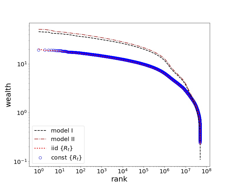
Refer to caption
Figure 3. The Zipf Plot
Refer to caption
Figure 4. The Lorenz Curve

We compare our models with two other models, in which {Rt}\{R_{t}\} is respectively an iid process and a constant.1818 18 In the former case, we set Nσ=1N_{\sigma}=1 in model I (so that σt\sigma_{t} reduces to its stationary mean) or Nμ=1N_{\mu}=1 in model II (so that μt\mu_{t} reduces to its stationary mean). In the latter case, we reduce {Rt}\{R_{t}\} to its stationary mean. The difference between the results of model I and model II and the results of the other two models reflects the role of stochastic volatility and mean persistence of the wealth return process. Parameter setups and results are reported in tables 1–2.1919 19 Since the standard Bewley-Ayagari-Hugget model does not generate fat-tailed wealth distribution (see, e.g., Stachurski and Toda 2018), calculating the tail exponent of the stationary wealth distribution when {Rt}\{R_{t}\} is a constant is relatively less standard. However, doing this allows us to reveal the effect of capital income risk on the tail thickness of the stationary wealth distribution.

As can be seen in table 1, the tail exponents of model I and model II are smaller than the tail exponents when {Rt}\{R_{t}\} is iid or constant. In other words, both stochastic volatility and mean persistence in wealth returns lead to a higher degree of wealth inequality. Moreover, mean persistence results in slightly lower tail exponents than stochastic volatility does.

Similarly, the Gini coefficients generated by model I and model II are much higher than those generated by the other two models, illustrating from another perspective that stochastic volatility and mean persistence of wealth returns cause more inequality in wealth. However, different from the previous case, compared with mean persistence, which generates a Gini index 0.45, stochastic volatility has a higher impact on wealth inequality, creating a Gini index 0.47.

Moreover, at least in the current models, iid wealth returns do not have obvious effect on wealth inequality, both in terms of their impact on the tail exponent and in terms of their impact on the Gini coefficient.

The above descriptions are further illustrated in table 2 and figures 3–4. In particular, in table 2 we calculate the wealth share of a given fraction of poorest agents. Notably, the top 10%10\% richest agents hold respectively 35.2%35.2\%, 34.3%34.3\%, 25.8%25.8\% and 25.7%25.7\% of the total wealth, while the poorest 10%10\% agents hold respectively 1.8%1.8\%, 2.4%2.4\%, 3.4%3.4\%, 3.5%3.5\% of the total wealth in the four model economies. In figure 3 we create the Zipf plot (i.e., plotting log\log wealth v.s. log\log rank). It is clearly indicated that model I and model II generate stationary wealth distributions with fatter upper tails than the other models do, and that the stationary wealth distribution of model II has the fattest upper tail. In figure 4 we plot the Lorenz curve, which can be viewed as a generalized graphical representation of table 2.

Finally, sensitivity analysis with respect to model parameters and a more detailed quantitative analysis can be found in the online appendix of this paper.

6. Appendix A: Proof of Section 3 Results

In proofs we let {ℱt}t≥0\{\mathscr{F}_{t}\}_{t\geq 0} be the natural filtration, where ℱt:=σ⁡(s0,⋯,st)\mathscr{F}_{t}:=\sigma(s_{0},\cdots,s_{t}) with st:=(at,zt)s_{t}:=(a_{t},z_{t}) for all tt. We start by proving the results of section 3.

Proof of example 3.1.

Note that for fixed n∈ℕn\in\mathbbm{N},

∥Kn∥=sup‖f‖≤1∥Knf∥=sup‖f‖≤1supz∈𝖹|𝔼zR1⋯Rnf(zn)|=supz∈𝖹𝔼zR1⋯Rn.\|K^{n}\|=\sup_{\|f\|\leq 1}\|K^{n}f\|=\sup_{\|f\|\leq 1}\sup_{z\in\mathsf{Z}}\left|\mathbbm{E}\,_{z}R_{1}\cdots R_{n}f(z_{n})\right|=\sup_{z\in\mathsf{Z}}\mathbbm{E}\,_{z}R_{1}\cdots R_{n}.

Suppose assumption 3.1 holds. Note that every t∈ℕt\in\mathbbm{N} can be written as t=k​n+ℓt=kn+\ell where k∈ℕ∪{0}k\in\mathbbm{N}\cup\{0\} and ℓ∈{0,⋯,n−1}\ell\in\{0,\cdots,n-1\}. Since ‖Kt‖=‖Kk​n+ℓ‖≤‖Kn‖k​‖Kℓ‖\|K^{t}\|=\|K^{kn+\ell}\|\leq\|K^{n}\|^{k}\|K^{\ell}\|,

‖Kt‖1/t=‖Kk​n+ℓ‖1/t≤‖Kn‖k/t​‖Kℓ‖1/t=‖Kn‖1n+ℓ/k​‖Kℓ‖1/t.\|K^{t}\|^{1/t}=\|K^{kn+\ell}\|^{1/t}\leq\|K^{n}\|^{k/t}\|K^{\ell}\|^{1/t}=\|K^{n}\|^{\frac{1}{n+\ell/k}}\|K^{\ell}\|^{1/t}.

Since β​‖Kn‖<1\beta\|K^{n}\|<1 by assumption 3.1 and ‖Kℓ‖≤‖K‖ℓ<∞\|K^{\ell}\|\leq\|K\|^{\ell}<\infty, letting t→∞t\to\infty (and thus k→∞k\to\infty) yields

β​r​(K)=β​limt→∞‖Kt‖1/t≤β​limk→∞‖Kn‖1n​nn+ℓ/k​‖Kℓ‖1k​n+ℓ=β​‖Kn‖1/n<1.\beta r(K)=\beta\lim_{t\to\infty}\|K^{t}\|^{1/t}\leq\beta\lim_{k\to\infty}\|K^{n}\|^{\frac{1}{n}\frac{n}{n+\ell/k}}\|K^{\ell}\|^{\frac{1}{kn+\ell}}=\beta\|K^{n}\|^{1/n}<1.

On the other hand, suppose β​r​(K)<1\beta r(K)<1. Then by the definition of rr there exists n∈ℕn\in\mathbbm{N} such that β​‖Kn‖1/n<1\beta\|K^{n}\|^{1/n}<1. Thus βn​‖Kn‖<1\beta^{n}\|K^{n}\|<1 and assumption 3.1 is verified. ∎

For the rest of this section, we let nn and θ\theta be defined as in assumption 3.1.

Proof of lemma 3.1.

Iterating backward on the maximal path (6), we can show that

a~t=(∏i=1tRi)​a+∑j=1t(Yj​∏i=j+1tRi).\tilde{a}_{t}=\left(\prod_{i=1}^{t}R_{i}\right)a+\sum_{j=1}^{t}\left(Y_{j}\,\prod_{i=j+1}^{t}R_{i}\right).

Taking discounted expectation yields

βt​𝔼a,z​a~t\displaystyle\beta^{t}\mathbbm{E}\,_{a,z}\tilde{a}_{t} =[𝔼z​(βt​∏i=1tRi)]​a+∑j=1t𝔼z​[(βt−j​∏i=j+1tRi)​(βj​Yj)].\displaystyle=\left[\mathbbm{E}\,_{z}\left(\beta^{t}\prod_{i=1}^{t}R_{i}\right)\right]a+\sum_{j=1}^{t}\mathbbm{E}\,_{z}\left[\left(\beta^{t-j}\prod_{i=j+1}^{t}R_{i}\right)\left(\beta^{j}Y_{j}\right)\right].

Let M⁡(a,z):=∑t≥0βt​𝔼a,z​a~tM(a,z):=\sum_{t\geq 0}\beta^{t}\mathbbm{E}\,_{a,z}\tilde{a}_{t}. Then the monotone convergence theorem and the Markov property imply that

M⁡(a,z)\displaystyle M(a,z) =∑t=0∞𝔼z​(βt​∏i=1tRi)​a+∑t=0∞∑j=1t𝔼z​[(βt−j​∏i=j+1tRi)​(βj​Yj)]\displaystyle=\sum_{t=0}^{\infty}\mathbbm{E}\,_{z}\left(\beta^{t}\prod_{i=1}^{t}R_{i}\right)a+\sum_{t=0}^{\infty}\sum_{j=1}^{t}\mathbbm{E}\,_{z}\left[\left(\beta^{t-j}\prod_{i=j+1}^{t}R_{i}\right)\left(\beta^{j}Y_{j}\right)\right]
=𝔼z​(∑t=0∞βt​∏i=1tRi)​a+∑j=1∞𝔼z​𝔼z​[(βj​Yj)​(∑i=0∞βi​∏k=1iRj+k)|ℱj]\displaystyle=\mathbbm{E}\,_{z}\left(\sum_{t=0}^{\infty}\beta^{t}\prod_{i=1}^{t}R_{i}\right)a+\sum_{j=1}^{\infty}\mathbbm{E}\,_{z}\mathbbm{E}\,_{z}\left[(\beta^{j}Y_{j})\left(\sum_{i=0}^{\infty}\beta^{i}\prod_{k=1}^{i}R_{j+k}\right)\Big|\mathscr{F}_{j}\right]
=𝔼z​(∑t=0∞βt​∏i=1tRi)​a+∑j=1∞𝔼z​[(βj​Yj)​𝔼zj​(∑i=0∞βi​∏k=1iRk)].\displaystyle=\mathbbm{E}\,_{z}\left(\sum_{t=0}^{\infty}\beta^{t}\prod_{i=1}^{t}R_{i}\right)a+\sum_{j=1}^{\infty}\mathbbm{E}\,_{z}\left[(\beta^{j}Y_{j})\,\mathbbm{E}\,_{z_{j}}\left(\sum_{i=0}^{\infty}\beta^{i}\prod_{k=1}^{i}R_{k}\right)\right].

By the Markov property and assumption 3.1, for all k∈ℕk\in\mathbbm{N} and z∈𝖹z\in\mathsf{Z}, we have

𝔼zβk​nR1⋯Rk​n\displaystyle\mathbbm{E}\,_{z}\beta^{kn}R_{1}\cdots R_{kn} =𝔼z𝔼z[β(k−1)​nR1⋯R(k−1)​nβnR(k−1)​n+1⋯Rk​n∣ℱ(k−1)​n]\displaystyle=\mathbbm{E}\,_{z}\mathbbm{E}\,_{z}[\beta^{(k-1)n}R_{1}\cdots R_{(k-1)n}\beta^{n}R_{(k-1)n+1}\cdots R_{kn}\mid\mathscr{F}_{(k-1)n}]
=𝔼zβ(k−1)​nR1⋯R(k−1)​n𝔼z(k−1)​n(βnR1⋯Rn)\displaystyle=\mathbbm{E}\,_{z}\beta^{(k-1)n}R_{1}\cdots R_{(k-1)n}\mathbbm{E}\,_{z_{(k-1)n}}(\beta^{n}R_{1}\cdots R_{n})
≤θ𝔼zβ(k−1)​nR1⋯R(k−1)​n≤⋯≤θk.\displaystyle\leq\theta\mathbbm{E}\,_{z}\beta^{(k-1)n}R_{1}\cdots R_{(k-1)n}\leq\cdots\leq\theta^{k}.

Taking supremum on both sides yields

(24) βk​nsupz∈𝖹𝔼zR1⋯Rk​n≤θk.\beta^{kn}\sup_{z\in\mathsf{Z}}\mathbbm{E}\,_{z}R_{1}\cdots R_{kn}\leq\theta^{k}.

Moreover, assumption 3.3 implies that K0:=supz∈𝖹𝔼z​R^<∞K_{0}:=\sup_{z\in\mathsf{Z}}\mathbbm{E}\,_{z}\hat{R}<\infty. Hence,

𝔼z(∑i=0n−1βiR1⋯Ri)\displaystyle\mathbbm{E}\,_{z}\left(\sum_{i=0}^{n-1}\beta^{i}R_{1}\cdots R_{i}\right) =∑i=0n−1βi𝔼zR1⋯Ri=∑i=0n−1βi𝔼zR1⋯Ri−1𝔼zi−1R1\displaystyle=\sum_{i=0}^{n-1}\beta^{i}\mathbbm{E}\,_{z}R_{1}\cdots R_{i}=\sum_{i=0}^{n-1}\beta^{i}\mathbbm{E}\,_{z}R_{1}\cdots R_{i-1}\mathbbm{E}\,_{z_{i-1}}R_{1}
≤∑i=0n−1βi𝔼zR1⋯Ri−1K0≤⋯≤∑i=0n−1βiK0i=:K1<∞\displaystyle\leq\sum_{i=0}^{n-1}\beta^{i}\mathbbm{E}\,_{z}R_{1}\cdots R_{i-1}K_{0}\leq\cdots\leq\sum_{i=0}^{n-1}\beta^{i}K_{0}^{i}=:K_{1}<\infty

for all z∈𝖹z\in\mathsf{Z}. Taking supremum on both sides yields

(25) supz∈𝖹𝔼z(∑i=0n−1βiR1⋯Ri)≤K1<∞.\sup_{z\in\mathsf{Z}}\mathbbm{E}\,_{z}\left(\sum_{i=0}^{n-1}\beta^{i}R_{1}\cdots R_{i}\right)\leq K_{1}<\infty.

Based on (24) and (25), we have

𝔼z​(∑i=0∞βi​∏k=1iRk)\displaystyle\mathbbm{E}\,_{z}\left(\sum_{i=0}^{\infty}\beta^{i}\prod_{k=1}^{i}R_{k}\right) =∑k=0∞𝔼z(∑i=0n−1βk​n+iR1⋯Rk​n+i)\displaystyle=\sum_{k=0}^{\infty}\mathbbm{E}\,_{z}\left(\sum_{i=0}^{n-1}\beta^{kn+i}R_{1}\cdots R_{kn+i}\right)
=∑k=0∞𝔼z[βk​nR1⋯Rk​n(∑i=0n−1βiRk​n+1⋯Rk​n+i)]\displaystyle=\sum_{k=0}^{\infty}\mathbbm{E}\,_{z}\left[\beta^{kn}R_{1}\cdots R_{kn}\left(\sum_{i=0}^{n-1}\beta^{i}R_{kn+1}\cdots R_{kn+i}\right)\right]
=∑k=0∞𝔼z[βk​nR1⋯Rk​n𝔼zk​n(∑i=0n−1βiR1⋯Ri)]\displaystyle=\sum_{k=0}^{\infty}\mathbbm{E}\,_{z}\left[\beta^{kn}R_{1}\cdots R_{kn}\mathbbm{E}\,_{z_{kn}}\left(\sum_{i=0}^{n-1}\beta^{i}R_{1}\cdots R_{i}\right)\right]
≤∑k=0∞𝔼zβk​nR1⋯Rk​nK1≤∑k=0∞θkK1:=K2<∞\displaystyle\leq\sum_{k=0}^{\infty}\mathbbm{E}\,_{z}\beta^{kn}R_{1}\cdots R_{kn}K_{1}\leq\sum_{k=0}^{\infty}\theta^{k}K_{1}:=K_{2}<\infty

for all z∈𝖹z\in\mathsf{Z}. Hence,

supz∈𝖹𝔼z​(∑i=0∞βi​∏k=1iRk)≤K2<∞.\sup_{z\in\mathsf{Z}}\mathbbm{E}\,_{z}\left(\sum_{i=0}^{\infty}\beta^{i}\prod_{k=1}^{i}R_{k}\right)\leq K_{2}<\infty.

Finally, assumption 3.2 implies that

M⁡(a,z)≤K2​a+K2​∑t=1∞βt​𝔼z​Yt<∞\displaystyle M(a,z)\leq K_{2}a+K_{2}\sum_{t=1}^{\infty}\beta^{t}\mathbbm{E}\,_{z}Y_{t}<\infty

for all (a,z)∈𝖲0(a,z)\in\mathsf{S}_{0}. This concludes the proof. ∎

Proof of theorem 3.1.

This result extends theorem 1 of Benhabib et al. 2015 and theorem 3.1 of Li and Stachurski 2014. While the assumptions are weaker in our setting, the proof is similar and hence omitted. ∎

In the next, we aim to prove proposition 3.1. To that end, we define ℋ\mathscr{H} to be the set of functions h:𝖲0→ℝh\colon\mathsf{S}_{0}\rightarrow\mathbbm{R} that satisfies

  1. (1)

    hh is continuous,

  2. (2)

    hh is decreasing in the first argument, and

  3. (3)

    ∃K∈ℝ\exists K\in\mathbbm{R} such that u′​(a)≤h⁡(a,z)≤u′​(a)+Ku^{\prime}(a)\leq h(a,z)\leq u^{\prime}(a)+K for all (a,z)∈𝖲0(a,z)\in\mathsf{S}_{0}.

On ℋ\mathscr{H} we impose the distance

(26) d∞​(h,g):=‖h−g‖:=sup(a,z)∈𝖲0|h⁡(a,z)−g⁡(a,z)|.d_{\infty}(h,g):=\left\|h-g\right\|:=\sup_{(a,z)\in\mathsf{S}_{0}}\left|h(a,z)-g(a,z)\right|.

While the elements of ℋ\mathscr{H} are not bounded, the function d∞d_{\infty} is a valid metric. Moreover, standard argument shows that (ℋ,d∞)(\mathscr{H},d_{\infty}) is a complete metric space.

Proof of proposition 3.1.

Standard argument shows that ρ\rho is a valid metric. To show completeness of (𝒞,ρ)(\mathscr{C},\rho), it suffices to show that (𝒞,ρ)(\mathscr{C},\rho) and (ℋ,d∞)(\mathscr{H},d_{\infty}) are isometrically isomorphic.

To see that this is so, let HH be the map on 𝒞\mathscr{C} defined by H​c=u′∘cHc=u^{\prime}\circ c. It is easy to show that H:𝒞→ℋH:\mathscr{C}\rightarrow\mathscr{H} and that it is a bijection. Moreover, for all c,d∈𝒞c,d\in\mathscr{C},

d∞​(H​c,H​d)=‖H​c−H​d‖=‖u′∘c−u′∘d‖=ρ⁡(c,d).d_{\infty}(Hc,Hd)=\left\|Hc-Hd\right\|=\left\|u^{\prime}\circ c-u^{\prime}\circ d\right\|=\rho(c,d).

Hence, HH is an isometry. The space (𝒞,ρ)(\mathscr{C},\rho) is then complete, as claimed. ∎

Proof of proposition 3.2.

Let cc be a policy in 𝒞\mathscr{C} satisfying (11). That cc satisfies the first order optimality conditions is immediate by definition. It remains to show that any asset path generated by cc satisfies the transversality condition (8). To see that this is so, observe that, by (10),

(27) 𝔼a,z​βt​(u′∘c)​(at,zt)​at≤βt​𝔼a,z​u′​(at)​at+βt​K​𝔼a,z​at.\mathbbm{E}\,_{a,z}\beta^{t}(u^{\prime}\circ c)(a_{t},z_{t})a_{t}\leq\beta^{t}\mathbbm{E}\,_{a,z}u^{\prime}(a_{t})a_{t}+\beta^{t}K\mathbbm{E}\,_{a,z}a_{t}.

Regarding the first term on the right hand side of (27), fix L>0L>0 and observe that

𝔼a,z​u′​(at)​at\displaystyle\mathbbm{E}\,_{a,z}u^{\prime}(a_{t})a_{t} =𝔼a,zu′(at)at𝟙{at≤L}+𝔼a,zu′(at)at𝟙{at>L}\displaystyle=\mathbbm{E}\,_{a,z}u^{\prime}(a_{t})a_{t}\mathbbm{1}\{a_{t}\leq L\}+\mathbbm{E}\,_{a,z}u^{\prime}(a_{t})a_{t}\mathbbm{1}\{a_{t}>L\}
≤L​𝔼a,z​u′​(at)+u′​(L)​𝔼a,z​at≤L​𝔼z​u′​(Yt)+u′​(L)​𝔼a,z​a~t,\displaystyle\leq L\mathbbm{E}\,_{a,z}u^{\prime}(a_{t})+u^{\prime}(L)\mathbbm{E}\,_{a,z}a_{t}\leq L\mathbbm{E}\,_{z}u^{\prime}(Y_{t})+u^{\prime}(L)\mathbbm{E}\,_{a,z}\tilde{a}_{t},

where a~t\tilde{a}_{t} is the maximal path defined in (6). We then have

(28) βt​𝔼a,z​u′​(at)​at≤L​βt​𝔼z​u′​(Yt)+u′​(L)​βt​𝔼a,z​a~t.\beta^{t}\mathbbm{E}\,_{a,z}u^{\prime}(a_{t})a_{t}\leq L\beta^{t}\mathbbm{E}\,_{z}u^{\prime}(Y_{t})+u^{\prime}(L)\beta^{t}\mathbbm{E}\,_{a,z}\tilde{a}_{t}.

Since M:=supz∈𝖹𝔼z​u′​(Y^)<∞M:=\sup_{z\in\mathsf{Z}}\mathbbm{E}\,_{z}u^{\prime}(\hat{Y})<\infty by assumption 3.3, the Markov property then implies that for all z∈𝖹z\in\mathsf{Z} and t≥1t\geq 1,

𝔼z​u′​(Yt)=𝔼z​𝔼z​[u′​(Yt)|ℱt−1]=𝔼z​𝔼zt−1​u′​(Y^)≤𝔼z​M=M.\mathbbm{E}\,_{z}u^{\prime}\left(Y_{t}\right)=\mathbbm{E}\,_{z}\mathbbm{E}\,_{z}\left[u^{\prime}\left(Y_{t}\right)\big|\mathscr{F}_{t-1}\right]=\mathbbm{E}\,_{z}\mathbbm{E}\,_{z_{t-1}}u^{\prime}(\hat{Y})\leq\mathbbm{E}\,_{z}M=M.

Hence, limt→∞βt​𝔼z​u′​(Yt)=0\lim_{t\to\infty}\beta^{t}\mathbbm{E}\,_{z}u^{\prime}\left(Y_{t}\right)=0. Since in addition limt→∞βt​𝔼a,z​a~t=0\lim_{t\to\infty}\beta^{t}\mathbbm{E}\,_{a,z}\tilde{a}_{t}=0 by lemma 3.1, (28) then implies that limt→∞βt​𝔼a,z​u′​(at)​at=0\lim_{t\to\infty}\beta^{t}\mathbbm{E}\,_{a,z}u^{\prime}(a_{t})a_{t}=0.

Moreover, the second term on the right hand side of (27) is dominated by βt​K​𝔼a,z​a~t\beta^{t}K\mathbbm{E}\,_{a,z}\tilde{a}_{t}, and converges to zero by lemma 3.1. We have thus shown that the term on the right hand side of (27) converges to zero. Hence, the transversality condition holds. ∎

Proof of proposition 3.3.

Fix c∈𝒞c\in\mathscr{C} and (a,z)∈𝖲0(a,z)\in\mathsf{S}_{0}. Because c∈𝒞c\in\mathscr{C}, the map ξ↦ψc​(ξ,a,z)\xi\mapsto\psi_{c}(\xi,a,z) is increasing. Since ξ↦u′​(ξ)\xi\mapsto u^{\prime}(\xi) is strictly decreasing, the equation (12) can have at most one solution. Hence uniqueness holds.

Existence follows from the intermediate value theorem provided we can show that

  1. (a)

    ξ↦ψc​(ξ,a,z)\xi\mapsto\psi_{c}(\xi,a,z) is a continuous function,

  2. (b)

    ∃ξ∈(0,a]\exists\xi\in(0,a] such that u′​(ξ)≥ψc​(ξ,a,z)u^{\prime}(\xi)\geq\psi_{c}(\xi,a,z), and

  3. (c)

    ∃ξ∈(0,a]\exists\xi\in(0,a] such that u′​(ξ)≤ψc​(ξ,a,z)u^{\prime}(\xi)\leq\psi_{c}(\xi,a,z).

For part (a), it suffices to show that g⁡(ξ):=𝔼z​R^​(u′∘c)​[R^​(a−ξ)+Y^,z^]g(\xi):=\mathbbm{E}\,_{z}\hat{R}\left(u^{\prime}\circ c\right)\left[\hat{R}(a-\xi)+\hat{Y},\hat{z}\right] is continuous on (0,a](0,a]. To this end, fix ξ∈(0,a]\xi\in(0,a] and ξn→ξ\xi_{n}\rightarrow\xi. By (10) we have

(29) R^​(u′∘c)​[R^​(a−ξ)+Y^,z^]≤R^​(u′∘c)​(Y^,z^)≤R^​u′​(Y^)+R^​K.\displaystyle\hat{R}\left(u^{\prime}\circ c\right)\left[\hat{R}\left(a-\xi\right)+\hat{Y},\hat{z}\right]\leq\hat{R}\left(u^{\prime}\circ c\right)(\hat{Y},\hat{z})\leq\hat{R}u^{\prime}(\hat{Y})+\hat{R}K.

The last term is integrable by assumption 3.3. Hence the dominated convergence theorem applies. From this fact and the continuity of cc, we obtain g⁡(ξn)→g⁡(ξ)g(\xi_{n})\rightarrow g(\xi). Hence, ξ↦ψc​(ξ,a,z)\xi\mapsto\psi_{c}(\xi,a,z) is continuous.

Part (b) clearly holds, since u′​(ξ)→∞u^{\prime}(\xi)\rightarrow\infty as ξ→0\xi\rightarrow 0 and ξ↦ψc​(ξ,a,z)\xi\mapsto\psi_{c}(\xi,a,z) is increasing and always finite (since it is continuous as shown in the previous paragraph). Part (c) is also trivial (just set ξ=a\xi=a). ∎

Proof of proposition 3.4.

Fix c∈𝒞c\in\mathscr{C}. With slight abuse of notation, we denote

g⁡(ξ,a,z):=𝔼z​R^​(u′∘c)​[R^​(a−ξ)+Y^,z^].g\left(\xi,a,z\right):=\mathbbm{E}\,_{z}\hat{R}\left(u^{\prime}\circ c\right)\left[\hat{R}\left(a-\xi\right)+\hat{Y},\,\hat{z}\right].

Step 1. We show that T​cTc is continuous. To apply a standard fixed point parametric continuity result such as theorem B.1.4 of Stachurski 2009, we first show that ψc\psi_{c} is jointly continuous on the set GG defined in (13). This will be true if gg is jointly continuous on GG. For any {(ξn,an,zn)}\{(\xi_{n},a_{n},z_{n})\} and (ξ,a,z)(\xi,a,z) in GG with (ξn,an,zn)→(ξ,a,z)(\xi_{n},a_{n},z_{n})\rightarrow(\xi,a,z), we need to show that g⁡(ξn,an,zn)→g⁡(ξ,a,z)g(\xi_{n},a_{n},z_{n})\rightarrow g(\xi,a,z). To that end, we define

h1​(ξ,a,z^,ζ^,η^),h2​(ξ,a,z^,ζ^,η^):=R^​[u′​(Y^)+K]±R^​(u′∘c)​[R^​(a−ξ)+Y^,z^],\displaystyle h_{1}(\xi,a,\hat{z},\hat{\zeta},\hat{\eta}),\,h_{2}(\xi,a,\hat{z},\hat{\zeta},\hat{\eta}):=\hat{R}[u^{\prime}(\hat{Y})+K]\pm\hat{R}\left(u^{\prime}\circ c\right)[\hat{R}\left(a-\xi\right)+\hat{Y},\hat{z}],

where R^:=R⁡(z^,ζ^)\hat{R}:=R(\hat{z},\hat{\zeta}) and Y^:=Y⁡(z^,η^)\hat{Y}:=Y(\hat{z},\hat{\eta}) as defined in (2.2). Then h1h_{1} and h2h_{2} are continuous in (ξ,a,z^)(\xi,a,\hat{z}) by the continuity of cc and assumption 3.4, and they are nonnegative since (29) implies that 0≤R^​(u′∘c)​[R^​(a−ξ)+Y^,z^]≤R^​[u′​(Y^)+K]0\leq\hat{R}\left(u^{\prime}\circ c\right)[\hat{R}\left(a-\xi\right)+\hat{Y},\hat{z}]\leq\hat{R}[u^{\prime}(\hat{Y})+K].

Moreover, since the stochastic kernel PP is Feller, the product measure satisfies2020 20 Here →\mathrel{{\mathop{\to}\limits}} denotes weak convergence, i.e., for all bounded continuous function ff, we have ∫f⁡(z^,ζ^,η^)​P​(zn,⁡𝑑z^)​ν​(⁡𝑑ζ^)​μ​(⁡𝑑η^)→∫f⁡(z^,ζ^,η^)​P​(z,⁡𝑑z^)​ν​(⁡𝑑ζ^)​μ​(⁡𝑑η^).\int f(\hat{z},\hat{\zeta},\hat{\eta})P(z_{n},\mathop{}\!\mathrm{d}\hat{z})\nu(\mathop{}\!\mathrm{d}\hat{\zeta})\mu(\mathop{}\!\mathrm{d}\hat{\eta})\to\int f(\hat{z},\hat{\zeta},\hat{\eta})P(z,\mathop{}\!\mathrm{d}\hat{z})\nu(\mathop{}\!\mathrm{d}\hat{\zeta})\mu(\mathop{}\!\mathrm{d}\hat{\eta}). The formal definition of weak convergence is provided in section 4.3.1.

P⁡(zn,⋅)⊗ν⊗μ⟶P⁡(z,⋅)⊗ν⊗μ.P(z_{n},\cdot)\otimes\nu\otimes\mu\mathrel{{\mathop{\longrightarrow}\limits}}P(z,\cdot)\otimes\nu\otimes\mu.

Based on the generalized Fatou’s lemma of Feinberg et al. 2014 (theorem 1.1),

lim infn→∞\displaystyle\liminf_{n\rightarrow\infty} ∫hi​(ξn,an,z^,ζ^,η^)​P​(zn,⁡𝑑z^)​ν​(⁡𝑑ζ^)​μ​(⁡𝑑η^)\displaystyle\int h_{i}(\xi_{n},a_{n},\hat{z},\hat{\zeta},\hat{\eta})P(z_{n},\mathop{}\!\mathrm{d}\hat{z})\nu(\mathop{}\!\mathrm{d}\hat{\zeta})\mu(\mathop{}\!\mathrm{d}\hat{\eta})
≥∫hi​(ξ,a,z^,ζ^,η^)​P​(z,⁡𝑑z^)​ν​(⁡𝑑ζ^)​μ​(⁡𝑑η^).\displaystyle\geq\int h_{i}(\xi,a,\hat{z},\hat{\zeta},\hat{\eta})P(z,\mathop{}\!\mathrm{d}\hat{z})\nu(\mathop{}\!\mathrm{d}\hat{\zeta})\mu(\mathop{}\!\mathrm{d}\hat{\eta}).

Since z↦𝔼z​R^​[u′​(Y^)+K]z\mapsto\mathbbm{E}\,_{z}\hat{R}\,[u^{\prime}(\hat{Y})+K] is continuous by assumption 3.4, this implies that

lim infn→∞(±𝔼zn​R^​(u′∘c)​[R^​(an−ξn)+Y^,z^])≥(±𝔼z​R^​(u′∘c)​[R^​(a−ξ)+Y^,z^]).\displaystyle\liminf_{n\rightarrow\infty}\left(\pm\mathbbm{E}\,_{z_{n}}\hat{R}\left(u^{\prime}\circ c\right)\left[\hat{R}\left(a_{n}-\xi_{n}\right)+\hat{Y},\hat{z}\right]\right)\geq\left(\pm\mathbbm{E}\,_{z}\hat{R}\left(u^{\prime}\circ c\right)\left[\hat{R}\left(a-\xi\right)+\hat{Y},\hat{z}\right]\right).

The function gg is then continuous since the above inequality is equivalent to

lim infn→∞g⁡(ξn,an,zn)≥g⁡(ξ,a,z)≥lim supn→∞g⁡(ξn,an,zn).\displaystyle\liminf_{n\rightarrow\infty}g(\xi_{n},a_{n},z_{n})\geq g(\xi,a,z)\geq\limsup_{n\rightarrow\infty}g(\xi_{n},a_{n},z_{n}).

Hence, ψc\psi_{c} is continuous on GG, as was to be shown. Moreover, since ξ↦ψc​(ξ,a,z)\xi\mapsto\psi_{c}(\xi,a,z) takes values in the closed interval

I⁡(a,z):=[u′​(a),u′​(a)+𝔼z​R^​(u′​(Y^)+K)],I(a,z):=\left[u^{\prime}(a),u^{\prime}(a)+\mathbbm{E}\,_{z}\hat{R}\left(u^{\prime}(\hat{Y})+K\right)\right],

the correspondence (a,z)↦I⁡(a,z)(a,z)\mapsto I(a,z) is nonempty, compact-valued and continuous. By theorem B.1.4 of Stachurski 2009, (a,z)↦[u′∘(T​c)]​(a,z)(a,z)\mapsto[u^{\prime}\circ(Tc)](a,z) is continuous. T​cTc is then continuous on 𝖲0\mathsf{S}_{0} since u′u^{\prime} is continuous.

Step 2. We show that T​cTc is increasing in aa. Suppose that for some z∈𝖹z\in\mathsf{Z} and a1,a2∈(0,∞)a_{1},a_{2}\in(0,\infty) with a1<a2a_{1}<a_{2}, we have ξ1:=T​c​(a1,z)>T​c​(a2,z)=:ξ2\xi_{1}:=Tc(a_{1},z)>Tc(a_{2},z)=:\xi_{2}. Since cc is increasing in aa by assumption, ψc\psi_{c} is increasing in ξ\xi and decreasing in aa. Then u′​(ξ1)<u′​(ξ2)=ψc​(ξ2,a2,z)≤ψc​(ξ1,a1,z)=u′​(ξ1)u^{\prime}(\xi_{1})<u^{\prime}(\xi_{2})=\psi_{c}(\xi_{2},a_{2},z)\leq\psi_{c}(\xi_{1},a_{1},z)=u^{\prime}(\xi_{1}). This is a contradiction.

Step 3. We have shown in proposition 3.3 that T​c​(a,z)∈(0,a]Tc(a,z)\in(0,a] for all (a,z)∈𝖲0(a,z)\in\mathsf{S}_{0}.

Step 4. We show that ‖u′∘(T​c)−u′‖<∞\|u^{\prime}\circ(Tc)-u^{\prime}\|<\infty. Since u′​[T​c​(a,z)]≥u′​(a)u^{\prime}[Tc(a,z)]\geq u^{\prime}(a), we have

|u′​[T​c​(a,z)]−u′​(a)|=u′​[T​c​(a,z)]−u′​(a)\displaystyle\left|u^{\prime}[Tc(a,z)]-u^{\prime}(a)\right|=u^{\prime}[Tc(a,z)]-u^{\prime}(a)
OPEN≤𝔼z​R^​(u′∘c)​(R^​[a−T​c​(a,z)]+Y^,z^))≤𝔼z​R^​[u′​(Y^)+K].\displaystyle\leq\mathbbm{E}\,_{z}\hat{R}\left(u^{\prime}\circ c\right)\left(\hat{R}\left[a-Tc(a,z)\right]+\hat{Y},\,\hat{z})\right)\leq\mathbbm{E}\,_{z}\hat{R}\left[u^{\prime}(\hat{Y})+K\right].

for all (a,z)∈𝖲0(a,z)\in\mathsf{S}_{0}. Assumption 3.3 then implies that

‖u′∘(T​c)−u′‖≤supz∈𝖹𝔼z​R^​u′​(Y^)+K⁡(supz∈𝖹𝔼z​R^)<∞.\displaystyle\left\|u^{\prime}\circ(Tc)-u^{\prime}\right\|\leq\sup_{z\in\mathsf{Z}}\mathbbm{E}\,_{z}\hat{R}u^{\prime}(\hat{Y})+K\left(\sup_{z\in\mathsf{Z}}\mathbbm{E}\,_{z}\hat{R}\right)<\infty.

This concludes the proof. ∎

In the rest of this section, we aim to prove theorem 3.2. Recall ℋ\mathscr{H} defined above. Given h∈ℋh\in\mathscr{H}, let T~​h\tilde{T}h be the function mapping (a,z)∈𝖲0(a,z)\in\mathsf{S}_{0} into the κ\kappa that solves

(30) κ=max⁡{β​𝔼z​R^​h​(R^​[a−(u′)−1​(κ)]+Y^,z^),u′​(a)}.\kappa=\max\left\{\beta\mathbbm{E}\,_{z}\hat{R}\,h\left(\hat{R}\left[a-\left(u^{\prime}\right)^{-1}(\kappa)\right]+\hat{Y},\,\hat{z}\right),\,u^{\prime}(a)\right\}.

The next lemma implies that T~\tilde{T} is a well-defined self-map on ℋ\mathscr{H}, as well as topologically conjugate to TT under the bijection H:𝒞→ℋH:\mathscr{C}\rightarrow\mathscr{H} defined by H​c:=u′∘cHc:=u^{\prime}\circ c.

Lemma 6.1.

The operator T~:ℋ→ℋ\tilde{T}\colon\mathscr{H}\to\mathscr{H} and satisfies T~​H=H​T\tilde{T}H=HT on 𝒞\mathscr{C}.

Proof of lemma 6.1.

Pick any c∈𝒞c\in\mathscr{C} and (a,z)∈𝖲0(a,z)\in\mathsf{S}_{0}. Let ξ:=T​c​(a,z)\xi:=Tc(a,z), then ξ\xi solves

(31) u′​(ξ)=max⁡{β​𝔼z​R^​(u′∘c)​[R^​(a−ξ)+Y^,z^],u′​(a)}.u^{\prime}(\xi)=\max\left\{\beta\mathbbm{E}\,_{z}\hat{R}\left(u^{\prime}\circ c\right)\left[\hat{R}\left(a-\xi\right)+\hat{Y},\,\hat{z}\right],\,u^{\prime}(a)\right\}.

We need to show that H​T​cHTc and T~​H​c\tilde{T}Hc evaluate to the same number at (a,z)(a,z). In other words, we need to show that u′​(ξ)u^{\prime}(\xi) is the solution to

κ=max⁡{β​𝔼z​R^​(u′∘c)​(R^​[a−(u′)−1​(κ)]+Y^,z^),u′​(a)}.\kappa=\max\left\{\beta\mathbbm{E}\,_{z}\hat{R}\left(u^{\prime}\circ c\right)\left(\hat{R}\left[a-\left(u^{\prime}\right)^{-1}(\kappa)\right]+\hat{Y},\,\hat{z}\right),\,u^{\prime}(a)\right\}.

But this is immediate from (31). Hence, we have shown that T~​H=H​T\tilde{T}H=HT on 𝒞\mathscr{C}. Since H:𝒞→ℋH\colon\mathscr{C}\to\mathscr{H} is a bijection, we have T~=H​T​H−1\tilde{T}=HTH^{-1}. Since in addition T:𝒞→𝒞T\colon\mathscr{C}\to\mathscr{C} by proposition 3.4, we have T~:ℋ→ℋ\tilde{T}\colon\mathscr{H}\to\mathscr{H}. This concludes the proof. ∎

Lemma 6.2.

T~\tilde{T} is order preserving on ℋ\mathscr{H}. That is, T~​h1≤T~​h2\tilde{T}h_{1}\leq\tilde{T}h_{2} for all h1,h2∈ℋh_{1},h_{2}\in\mathscr{H} with h1≤h2h_{1}\leq h_{2}.

Proof of lemma 6.2.

Let h1,h2h_{1},h_{2} be functions in ℋ\mathscr{H} with h1≤h2h_{1}\leq h_{2}. Suppose to the contrary that there exists (a,z)∈𝖲0(a,z)\in\mathsf{S}_{0} such that κ1:=T~​h1​(a,z)>T~​h2​(a,z)=:κ2\kappa_{1}:=\tilde{T}h_{1}(a,z)>\tilde{T}h_{2}(a,z)=:\kappa_{2}. Since functions in ℋ\mathscr{H} are decreasing in the first argument, we have

κ1\displaystyle\kappa_{1} =max⁡{β​𝔼z​R^​h1​(R^​[a−(u′)−1​(κ1)]+Y^,z^),u′​(a)}\displaystyle=\max\left\{\beta\mathbbm{E}\,_{z}\hat{R}\,h_{1}\left(\hat{R}\left[a-(u^{\prime})^{-1}(\kappa_{1})\right]+\hat{Y},\,\hat{z}\right),\,u^{\prime}(a)\right\}
≤max⁡{β​𝔼z​R^​h2​(R^​[a−(u′)−1​(κ1)]+Y^,z^),u′​(a)}\displaystyle\leq\max\left\{\beta\mathbbm{E}\,_{z}\hat{R}\,h_{2}\left(\hat{R}\left[a-(u^{\prime})^{-1}(\kappa_{1})\right]+\hat{Y},\,\hat{z}\right),\,u^{\prime}(a)\right\}
≤max⁡{β​𝔼z​R^​h2​(R^​[a−(u′)−1​(κ2)]+Y^,z^),u′​(a)}=κ2.\displaystyle\leq\max\left\{\beta\mathbbm{E}\,_{z}\hat{R}\,h_{2}\left(\hat{R}\left[a-(u^{\prime})^{-1}(\kappa_{2})\right]+\hat{Y},\,\hat{z}\right),\,u^{\prime}(a)\right\}=\kappa_{2}.

This is a contradiction. Hence, T~\tilde{T} is order preserving. ∎

Lemma 6.3.

T~n\tilde{T}^{n} is a contraction mapping on (ℋ,d∞)(\mathscr{H},d_{\infty}) with modulus θ\theta.

Proof of lemma 6.3.

Since T~\tilde{T} is order preserving and ℋ\mathscr{H} is closed under the addition of nonnegative constants, based on Blackwell 1965, it remains to verify: for nn and θ\theta given by assumption 3.1,

T~n​(h+γ)≤T~n​h+θ​γ​ for all ​h∈ℋ​ and ​γ≥0.\tilde{T}^{n}(h+\gamma)\leq\tilde{T}^{n}h+\theta\gamma\;\text{ for all }h\in\mathscr{H}\text{ and }\gamma\geq 0.

To that end, by assumption 3.1, it suffices to show that for all k∈ℕk\in\mathbbm{N} and (a,z)∈𝖲0(a,z)\in\mathsf{S}_{0},

(32) T~k(h+γ)(a,z)≤T~kh(a,z)+γβk𝔼zR1⋯Rk.\tilde{T}^{k}(h+\gamma)(a,z)\leq\tilde{T}^{k}h(a,z)+\gamma\beta^{k}\mathbbm{E}\,_{z}R_{1}\cdots R_{k}.

Fix h∈ℋh\in\mathscr{H}, γ≥0\gamma\geq 0, and let hγ​(a,z):=h⁡(a,z)+γh_{\gamma}(a,z):=h(a,z)+\gamma. By the definition of T~\tilde{T}, we have

T~​hγ​(a,z)\displaystyle\tilde{T}h_{\gamma}(a,z) =max⁡{β​𝔼z​R^​hγ​(R^​[a−(u′)−1​(T~​hγ)​(a,z)]+Y^,z^),u′​(a)}\displaystyle=\max\left\{\beta\mathbbm{E}\,_{z}\hat{R}\,h_{\gamma}\left(\hat{R}\left[a-(u^{\prime})^{-1}(\tilde{T}h_{\gamma})(a,z)\right]+\hat{Y},\hat{z}\right),u^{\prime}(a)\right\}
≤max⁡{β​𝔼z​R^​h​(R^​[a−(u′)−1​(T~​hγ)​(a,z)]+Y^,z^),u′​(a)}+γ​β​𝔼z​R1\displaystyle\leq\max\left\{\beta\mathbbm{E}\,_{z}\hat{R}\,h\left(\hat{R}\left[a-(u^{\prime})^{-1}(\tilde{T}h_{\gamma})(a,z)\right]+\hat{Y},\hat{z}\right),u^{\prime}(a)\right\}+\gamma\beta\mathbbm{E}\,_{z}R_{1}
≤max⁡{β​𝔼z​R^​h​(R^​[a−(u′)−1​(T~​h)​(a,z)]+Y^,z^),u′​(a)}+γ​β​𝔼z​R1.\displaystyle\leq\max\left\{\beta\mathbbm{E}\,_{z}\hat{R}\,h\left(\hat{R}\left[a-(u^{\prime})^{-1}(\tilde{T}h)(a,z)\right]+\hat{Y},\hat{z}\right),u^{\prime}(a)\right\}+\gamma\beta\mathbbm{E}\,_{z}R_{1}.

Here, the first inequality is elementary and the second is due to the fact that h≤hγh\leq h_{\gamma} and T~\tilde{T} is order preserving. Hence, T~​(h+γ)​(a,z)≤T~​h​(a,z)+γ​β​𝔼z​R1\tilde{T}(h+\gamma)(a,z)\leq\tilde{T}h(a,z)+\gamma\beta\mathbbm{E}\,_{z}R_{1} and (32) holds for k=1k=1. Suppose that (32) holds for arbitrary kk. It remains to show that (32) holds for k+1k+1. Define

f(z):=γβk𝔼zR1⋯Rk.f(z):=\gamma\beta^{k}\mathbbm{E}\,_{z}R_{1}\cdots R_{k}.

By the induction hypothesis, the monotonicity of T~\tilde{T} and the Markov property,

T~k+1​hγ​(a,z)\displaystyle\tilde{T}^{k+1}h_{\gamma}(a,z) =max⁡{β​𝔼z​R^​(T~k​hγ)​(R^​[a−(u′)−1​(T~k+1​hγ)​(a,z)]+Y^,z^),u′​(a)}\displaystyle=\max\left\{\beta\mathbbm{E}\,_{z}\hat{R}\,(\tilde{T}^{k}h_{\gamma})\left(\hat{R}\left[a-(u^{\prime})^{-1}(\tilde{T}^{k+1}h_{\gamma})(a,z)\right]+\hat{Y},\hat{z}\right),u^{\prime}(a)\right\}
≤max⁡{β​𝔼z​R^​(T~k​h+f)​(R^​[a−(u′)−1​(T~k+1​hγ)​(a,z)]+Y^,z^),u′​(a)}\displaystyle\leq\max\left\{\beta\mathbbm{E}\,_{z}\hat{R}\left(\tilde{T}^{k}h+f\right)\left(\hat{R}\left[a-(u^{\prime})^{-1}(\tilde{T}^{k+1}h_{\gamma})(a,z)\right]+\hat{Y},\hat{z}\right),u^{\prime}(a)\right\}
≤max⁡{β​𝔼z​R^​(T~k​h)​(R^​[a−(u′)−1​(T~k+1​hγ)​(a,z)]+Y^,z^),u′​(a)}\displaystyle\leq\max\left\{\beta\mathbbm{E}\,_{z}\hat{R}(\tilde{T}^{k}h)\left(\hat{R}\left[a-(u^{\prime})^{-1}(\tilde{T}^{k+1}h_{\gamma})(a,z)\right]+\hat{Y},\hat{z}\right),u^{\prime}(a)\right\}
+β​𝔼z​R1​f​(z1)\displaystyle\quad+\beta\mathbbm{E}\,_{z}R_{1}f(z_{1})
≤max⁡{β​𝔼z​R^​(T~k​h)​(R^​[a−(u′)−1​(T~k+1​h)​(a,z)]+Y^,z^),u′​(a)}\displaystyle\leq\max\left\{\beta\mathbbm{E}\,_{z}\hat{R}(\tilde{T}^{k}h)\left(\hat{R}\left[a-(u^{\prime})^{-1}(\tilde{T}^{k+1}h)(a,z)\right]+\hat{Y},\hat{z}\right),u^{\prime}(a)\right\}
+γβk+1𝔼zR1𝔼z1R1⋯Rk\displaystyle\quad+\gamma\beta^{k+1}\mathbbm{E}\,_{z}R_{1}\mathbbm{E}\,_{z_{1}}R_{1}\cdots R_{k}
=T~k+1h(a,z)+γβk+1𝔼zR1⋯Rk+1.\displaystyle=\tilde{T}^{k+1}h(a,z)+\gamma\beta^{k+1}\mathbbm{E}\,_{z}R_{1}\cdots R_{k+1}.

Hence, (32) is verified by induction. This concludes the proof. ∎

With the results established above, we are now ready to prove theorem 3.2.

Proof of theorem 3.2.

In view of propositions 3.1 and 3.2, to establish all the claims in theorem 3.2, we need only show that

ρ⁡(Tn​c,Tn​d)≤θ​ρ​(c,d)for all ​c,d∈𝒞.\rho(T^{n}c,T^{n}d)\leq\theta\rho(c,d)\quad\text{for all }\,c,d\in\mathscr{C}.

To this end, pick any c,d∈𝒞c,d\in\mathscr{C}. Note that the topological conjugacy result established in lemma 6.1 implies that T~=H​T​H−1\tilde{T}=HTH^{-1}. Hence,

T~n=(HTH−1)⋯(HTH−1)=HTnH−1andT~nH=HTn.\tilde{T}^{n}=(HTH^{-1})\cdots(HTH^{-1})=HT^{n}H^{-1}\quad\text{and}\quad\tilde{T}^{n}H=HT^{n}.

By the definition of ρ\rho and the contraction property established in lemma 6.3,

ρ⁡(Tn​c,Tn​d)=d∞​(H​Tn​c,H​Tn​d)=d∞​(T~n​H​c,T~n​H​d)≤θ​d∞​(H​c,H​d).\rho(T^{n}c,T^{n}d)=d_{\infty}(HT^{n}c,HT^{n}d)=d_{\infty}(\tilde{T}^{n}Hc,\tilde{T}^{n}Hd)\leq\theta d_{\infty}(Hc,Hd).

The right hand side is just θ​ρ​(c,d)\theta\rho(c,d), which completes the proof. ∎

7. Appendix B: Proof of Section 4 Results

Before working into the results of each subsection, we prove a general lemma that is frequently used in later sections. Recall that, for all c∈𝒞c\in\mathscr{C}, the value ξ⁡(a,z):=T​c​(a,z)\xi(a,z):=Tc(a,z) solves

(33) (u′∘ξ)​(a,z)=max⁡{β​𝔼z​R^​(u′∘c)​(R^​[a−ξ⁡(a,z)]+Y^,z^),u′​(a)}.\left(u^{\prime}\circ\xi\right)(a,z)=\max\left\{\beta\mathbbm{E}\,_{z}\hat{R}\left(u^{\prime}\circ c\right)\left(\hat{R}\left[a-\xi(a,z)\right]+\hat{Y},\,\hat{z}\right),\,u^{\prime}(a)\right\}.

Let c∗∈𝒞c^{*}\in\mathscr{C} denote the optimal policy. For each z∈𝖹z\in\mathsf{Z} and c∈𝒞c\in\mathscr{C}, define

(34) a¯c​(z):=(u′)−1​[β​𝔼z​R^​(u′∘c)​(Y^,z^)]anda¯​(z):=a¯c∗​(z).\bar{a}_{c}(z):=\left(u^{\prime}\right)^{-1}\left[\beta\mathbbm{E}\,_{z}\hat{R}\left(u^{\prime}\circ c\right)(\hat{Y},\,\hat{z})\right]\quad\text{and}\quad\bar{a}(z):=\bar{a}_{c^{*}}(z).

The next result implies that the borrowing constraint binds if and only if wealth is below a certain threshold level.

Lemma 7.1.

For all c∈𝒞c\in\mathscr{C}, T​c​(a,z)=aTc(a,z)=a if and only if a≤a¯c​(z)a\leq\bar{a}_{c}(z). In particular, c∗​(a,z)=ac^{*}(a,z)=a if and only if a≤a¯​(z)a\leq\bar{a}(z).

Proof of lemma 7.1.

Let a≤a¯c​(z)a\leq\bar{a}_{c}(z). We claim that ξ⁡(a,z)=a\xi(a,z)=a. Suppose to the contrary that ξ⁡(a,z)<a\xi(a,z)<a. Then (u′∘ξ)​(a,z)>u′​(a)(u^{\prime}\circ\xi)(a,z)>u^{\prime}(a). In view of (33), we have

u′​(a)<β​𝔼z​R^​(u′∘c)​(R^​[a−ξ⁡(a,z)]+Y^,z^)≤β​𝔼z​R^​(u′∘c)​(Y^,z^)=u′​[a¯c​(z)].\displaystyle u^{\prime}(a)<\beta\mathbbm{E}\,_{z}\hat{R}\left(u^{\prime}\circ c\right)\left(\hat{R}\left[a-\xi(a,z)\right]+\hat{Y},\,\hat{z}\right)\leq\beta\mathbbm{E}\,_{z}\hat{R}\left(u^{\prime}\circ c\right)(\hat{Y},\hat{z})=u^{\prime}[\bar{a}_{c}(z)].

From this we get a>a¯c​(z)a>\bar{a}_{c}(z), which is a contradiction. Hence, ξ⁡(a,z)=a\xi(a,z)=a.

On the other hand, if ξ⁡(a,z)=a\xi(a,z)=a, then (u′∘ξ)​(a,z)=u′​(a)(u^{\prime}\circ\xi)(a,z)=u^{\prime}(a). By (33), we have

u′​(a)≥β​𝔼z​R^​(u′∘c)​(Y^,z^)=u′​[a¯c​(z)].\displaystyle u^{\prime}(a)\geq\beta\mathbbm{E}\,_{z}\hat{R}\left(u^{\prime}\circ c\right)(\hat{Y},\,\hat{z})=u^{\prime}[\bar{a}_{c}(z)].

Hence, a≤a¯c​(z)a\leq\bar{a}_{c}(z). The first claim is verified. The second claim follows immediately from the first claim and the fact that c∗c^{*} is the unique fixed point of TT in 𝒞\mathscr{C}. ∎

Given c∈𝒞c\in\mathscr{C}, lemma 7.1 implies that ξ⁡(a,z):=T​c​(a,z)=a\xi(a,z):=Tc(a,z)=a for a≤a¯c​(z)a\leq\bar{a}_{c}(z), and that for a>a¯c​(z)a>\bar{a}_{c}(z), ξ⁡(a,z)\xi(a,z) solves

(u′∘ξ)​(a,z)=β​𝔼z​R^​(u′∘c)​(R^​[a−ξ⁡(a,z)]+Y^,z^).(u^{\prime}\circ\xi)(a,z)=\beta\mathbbm{E}\,_{z}\hat{R}\left(u^{\prime}\circ c\right)\left(\hat{R}\left[a-\xi(a,z)\right]+\hat{Y},\,\hat{z}\right).

7.1. Proof of section 4.1 results

Our first goal is to prove proposition 4.1. To that end, recall α\alpha given by assumption 4.1, and define the subspace 𝒞1\mathscr{C}_{1} as

(35) 𝒞1:={c∈𝒞:c⁡(a,z)a≥αfor all (a,z)∈𝖲0}.\mathscr{C}_{1}:=\left\{c\in\mathscr{C}:\frac{c(a,z)}{a}\geq\alpha\quad\text{for all }(a,z)\in\mathsf{S}_{0}\right\}.
Lemma 7.2.

𝒞1\mathscr{C}_{1} is a closed subset of 𝒞\mathscr{C}, and T​c∈𝒞1Tc\in\mathscr{C}_{1} for all c∈𝒞1c\in\mathscr{C}_{1}.

Proof of lemma 7.2.

To see that 𝒞1\mathscr{C}_{1} is closed, for a given sequence {cn}\{c_{n}\} in 𝒞1\mathscr{C}_{1} and c∈𝒞c\in\mathscr{C} with ρ⁡(cn,c)→0\rho(c_{n},c)\rightarrow 0, we need to verify that c∈𝒞1c\in\mathscr{C}_{1}. This obviously holds since cn​(a,z)/a≥αc_{n}(a,z)/a\geq\alpha for all nn and (a,z)∈𝖲0(a,z)\in\mathsf{S}_{0}, and, on the other hand, ρ⁡(cn,c)→0\rho(c_{n},c)\rightarrow 0 implies that cn​(a,z)→c⁡(a,z)c_{n}(a,z)\to c(a,z) for all (a,z)∈𝖲0(a,z)\in\mathsf{S}_{0}.

We next show that TT is a self-map on 𝒞1\mathscr{C}_{1}. Fix c∈𝒞1c\in\mathscr{C}_{1}. We have T​c∈𝒞Tc\in\mathscr{C} since TT is a self-map on 𝒞\mathscr{C}. It remains to show that ξ:=T​c\xi:=Tc satisfies ξ⁡(a,z)≥α​a\xi(a,z)\geq\alpha a for all (a,z)∈𝖲0(a,z)\in\mathsf{S}_{0}. Suppose to the contrary that ξ⁡(a,z)<α​a\xi(a,z)<\alpha a for some (a,z)∈𝖲0(a,z)\in\mathsf{S}_{0}. Then

u′​(α​a)<(u′∘ξ)​(a,z)=max⁡{β​𝔼z​R^​(u′∘c)​(R^​[a−ξ⁡(a,z)]+Y^,z^),u′​(a)}.u^{\prime}(\alpha a)<(u^{\prime}\circ\xi)(a,z)=\max\left\{\beta\mathbbm{E}\,_{z}\hat{R}\left(u^{\prime}\circ c\right)\left(\hat{R}\left[a-\xi(a,z)\right]+\hat{Y},\,\hat{z}\right),u^{\prime}(a)\right\}.

Since u′​(α​a)>u′​(a)u^{\prime}(\alpha a)>u^{\prime}(a) and c∈𝒞1c\in\mathscr{C}_{1}, this implies that

u′​(α​a)\displaystyle u^{\prime}(\alpha a) <β​𝔼z​R^​(u′∘c)​(R^​[a−ξ⁡(a,z)]+Y^,z^)\displaystyle<\beta\mathbbm{E}\,_{z}\hat{R}\left(u^{\prime}\circ c\right)\left(\hat{R}\left[a-\xi(a,z)\right]+\hat{Y},\,\hat{z}\right)
≤β​𝔼z​R^​u′​(α​R^​[a−ξ⁡(a,z)]+α​Y^)\displaystyle\leq\beta\mathbbm{E}\,_{z}\hat{R}u^{\prime}\left(\alpha\hat{R}\left[a-\xi(a,z)\right]+\alpha\hat{Y}\right)
≤β​𝔼z​R^​u′​[α​R^​(1−α)​a+α​Y^]≤β​𝔼z​R^​u′​[R^​(1−α)​(α​a)].\displaystyle\leq\beta\mathbbm{E}\,_{z}\hat{R}u^{\prime}\left[\alpha\hat{R}(1-\alpha)a+\alpha\hat{Y}\right]\leq\beta\mathbbm{E}\,_{z}\hat{R}\,u^{\prime}\left[\hat{R}(1-\alpha)(\alpha a)\right].

This is a contradicted with condition (1) of assumption 4.1 since (α​a,z)∈𝖲0(\alpha a,z)\in\mathsf{S}_{0}. Hence, ξ⁡(a,z)/a≥α\xi(a,z)/a\geq\alpha for all (a,z)∈𝖲0(a,z)\in\mathsf{S}_{0} and we conclude that T​c∈𝒞1Tc\in\mathscr{C}_{1}. ∎

With this result, we are now ready to prove proposition 4.1.

Proof of proposition 4.1.

Since the claim obviously holds when a=0a=0, it remains to verify that this claim holds on 𝖲0\mathsf{S}_{0}. We have shown in theorem 3.2 that TT is a contraction mapping on the complete metric space (𝒞,ρ)(\mathscr{C},\rho), with unique fixed point c∗c^{*}. Since in addition 𝒞1\mathscr{C}_{1} is a closed subset of 𝒞\mathscr{C} and T​𝒞1⊂𝒞1T\mathscr{C}_{1}\subset\mathscr{C}_{1} by lemma 7.2, we know that c∗∈𝒞1c^{*}\in\mathscr{C}_{1}. In summary, we have c∗​(a,z)≥α​ac^{*}(a,z)\geq\alpha a for all (a,z)∈𝖲(a,z)\in\mathsf{S}. ∎

Our next goal is to prove theorem 4.1. To that end, recall the integer nn given by the second condition of assumption 4.1.

Lemma 7.3.

supt≥0𝔼a,z​at<∞\sup_{t\geq 0}\mathbbm{E}\,_{a,z}\,a_{t}<\infty for all (a,z)∈𝖲(a,z)\in\mathsf{S}.

Proof of lemma 7.3.

Since c∗​(0,z)=0c^{*}(0,z)=0, proposition 4.1 implies that c∗​(a,z)≥α​ac^{*}(a,z)\geq\alpha a for all (a,z)∈𝖲(a,z)\in\mathsf{S}. For all t≥1t\geq 1, we have t=k​n+jt=kn+j in general, where k∈{0}∪ℕk\in\{0\}\cup\mathbbm{N} and j∈{0,1,⋯,n−1}j\in\{0,1,\cdots,n-1\}. Using these facts and (2.2), we have:

at\displaystyle a_{t} =Rt​(at−1−ct−1)+Yt≤(1−α)​Rt​at−1+Yt≤⋯\displaystyle=R_{t}(a_{t-1}-c_{t-1})+Y_{t}\leq(1-\alpha)R_{t}a_{t-1}+Y_{t}\leq\cdots
≤(1−α)tRt⋯R1a+(1−α)t−1Rt⋯R2Y1+⋯+(1−α)RtYt−1+Yt\displaystyle\leq(1-\alpha)^{t}R_{t}\cdots R_{1}a+(1-\alpha)^{t-1}R_{t}\cdots R_{2}Y_{1}+\cdots+(1-\alpha)R_{t}Y_{t-1}+Y_{t}
=(1−α)k​n+jRk​n+j⋯R1a+∑ℓ=1j(1−α)k​n+j−ℓRk​n+j⋯Rℓ+1Yℓ\displaystyle=(1-\alpha)^{kn+j}R_{kn+j}\cdots R_{1}a+\sum_{\ell=1}^{j}(1-\alpha)^{kn+j-\ell}R_{kn+j}\cdots R_{\ell+1}Y_{\ell}
+∑m=1k∑ℓ=1n(1−α)m​n−ℓRk​n+j⋯R(k−m)​n+j+ℓ+1Y(k−m)​n+j+ℓ\displaystyle\quad+\sum_{m=1}^{k}\sum_{\ell=1}^{n}(1-\alpha)^{mn-\ell}R_{kn+j}\cdots R_{(k-m)n+j+\ell+1}Y_{(k-m)n+j+\ell}

with probability one. Hence,

𝔼a,z​at\displaystyle\mathbbm{E}\,_{a,z}a_{t} ≤(1−α)t𝔼zRt⋯R1a+∑ℓ=1t(1−α)t−ℓ𝔼zRt⋯Rℓ+1Yℓ\displaystyle\leq(1-\alpha)^{t}\mathbbm{E}\,_{z}R_{t}\cdots R_{1}a+\sum_{\ell=1}^{t}(1-\alpha)^{t-\ell}\mathbbm{E}\,_{z}R_{t}\cdots R_{\ell+1}Y_{\ell}
=(1−α)k​n+j𝔼zRk​n+j⋯R1a+∑ℓ=1j(1−α)k​n+j−ℓ𝔼zRk​n+j⋯Rℓ+1Yℓ\displaystyle=(1-\alpha)^{kn+j}\mathbbm{E}\,_{z}R_{kn+j}\cdots R_{1}a+\sum_{\ell=1}^{j}(1-\alpha)^{kn+j-\ell}\mathbbm{E}\,_{z}R_{kn+j}\cdots R_{\ell+1}Y_{\ell}
+∑m=1k∑ℓ=1n(1−α)m​n−ℓ𝔼zRk​n+j⋯R(k−m)​n+j+ℓ+1Y(k−m)​n+j+ℓ\displaystyle\quad+\sum_{m=1}^{k}\sum_{\ell=1}^{n}(1-\alpha)^{mn-\ell}\mathbbm{E}\,_{z}R_{kn+j}\cdots R_{(k-m)n+j+\ell+1}Y_{(k-m)n+j+\ell}

for all (a,z)∈𝖲(a,z)\in\mathsf{S}. Define

γ:=(1−α)nsupz∈𝖹𝔼zR1⋯RnandM:=max1≤ℓ≤n[(1−α)ℓsupz∈𝖹𝔼zRℓ⋯R1].\gamma:=(1-\alpha)^{n}\sup_{z\in\mathsf{Z}}\mathbbm{E}\,_{z}R_{1}\cdots R_{n}\quad\text{and}\quad M:=\max_{1\leq\ell\leq n}\left[(1-\alpha)^{\ell}\sup_{z\in\mathsf{Z}}\mathbbm{E}\,_{z}R_{\ell}\cdots R_{1}\right].

Note that γ<1\gamma<1 by assumption 4.1-(2) and M<∞M<\infty by assumption 3.3 and the Markov property. Moreover, M′:=supt≥1𝔼z​Yt<∞M^{\prime}:=\sup_{t\geq 1}\mathbbm{E}\,_{z}Y_{t}<\infty by assumption 4.2. The Markov property then implies that for all (a,z)∈𝖲(a,z)\in\mathsf{S} and t≥0t\geq 0,

𝔼a,z​at\displaystyle\mathbbm{E}\,_{a,z}a_{t} ≤γk(1−α)j𝔼zRj⋯R1a+γk∑ℓ=1j(1−α)j−ℓ𝔼zRj⋯Rℓ+1Yℓ\displaystyle\leq\gamma^{k}(1-\alpha)^{j}\mathbbm{E}\,_{z}R_{j}\cdots R_{1}a+\gamma^{k}\sum_{\ell=1}^{j}(1-\alpha)^{j-\ell}\mathbbm{E}\,_{z}R_{j}\cdots R_{\ell+1}Y_{\ell}
+∑m=0k−1γm∑ℓ=1n(1−α)n−ℓ𝔼zR(k−m)​n+j⋯R(k−m−1)​n+j+ℓ+1Y(k−m)​n+j+ℓ\displaystyle\quad+\sum_{m=0}^{k-1}\gamma^{m}\sum_{\ell=1}^{n}(1-\alpha)^{n-\ell}\mathbbm{E}\,_{z}R_{(k-m)n+j}\cdots R_{(k-m-1)n+j+\ell+1}Y_{(k-m)n+j+\ell}
≤γk​M​a+γk​M​∑ℓ=1j𝔼z​Yℓ+∑m=0k−1γm​M​∑ℓ=1n𝔼z​Y(k−m−1)​n+j+ℓ\displaystyle\leq\gamma^{k}Ma+\gamma^{k}M\sum_{\ell=1}^{j}\mathbbm{E}\,_{z}Y_{\ell}+\sum_{m=0}^{k-1}\gamma^{m}M\sum_{\ell=1}^{n}\mathbbm{E}\,_{z}Y_{(k-m-1)n+j+\ell}
≤M​a+M​M′​n+∑m=0∞γm​M​M′​n<∞.\displaystyle\leq Ma+MM^{\prime}n+\sum_{m=0}^{\infty}\gamma^{m}MM^{\prime}n<\infty.

Hence, supt≥0𝔼a,z​at<∞\sup_{t\geq 0}\mathbbm{E}\,_{a,z}\,a_{t}<\infty for all (a,z)∈𝖲(a,z)\in\mathsf{S}, as was claimed. ∎

A function w∗:𝖲→ℝ+w^{*}\colon\mathsf{S}\to\mathbbm{R}_{+} is called norm-like if all its sublevel sets (i.e., sets of the form {s∈𝖲:w⁡(s)≤b},b∈ℝ+\{s\in\mathsf{S}\colon w(s)\leq b\},b\in\mathbbm{R}_{+}) are precompact in 𝖲\mathsf{S} (i.e., any sequence in a given sublevel set has a subsequence that converges to a point of 𝖲\mathsf{S}).

Proof of theorem 4.1.

Based on lemma D.5.3 of Meyn and Tweedie 2009, a stochastic kernel QQ is bounded in probability if and only if for all s∈𝖲s\in\mathsf{S}, there exists a norm-like function ws∗:𝖲→ℝ+w_{s}^{*}\colon\mathsf{S}\to\mathbbm{R}_{+} such that the (Q,s)(Q,s)-Markov process {st}t≥0\{s_{t}\}_{t\geq 0} satisfies lim supt→∞𝔼s​[ws∗​(st)]<∞\limsup_{t\to\infty}\mathbbm{E}\,_{s}\left[w_{s}^{*}(s_{t})\right]<\infty.

Fix (a,z)∈𝖲(a,z)\in\mathsf{S}. Since PP is bounded in probability by assumption 4.3, there exists a norm-like function w:𝖹→ℝ+w\colon\mathsf{Z}\to\mathbbm{R}_{+} such that lim supt→∞𝔼z​w​(zt)<∞\limsup_{t\to\infty}\mathbbm{E}\,_{z}w(z_{t})<\infty. Then w∗:𝖲→ℝ+w^{*}\colon\mathsf{S}\rightarrow\mathbbm{R}_{+} defined by w∗​(a0,z0):=a0+w⁡(z0)w^{*}(a_{0},z_{0}):=a_{0}+w(z_{0}) is a norm-like function on 𝖲\mathsf{S}. The stochastic kernel QQ is then bounded in probability since lemma 7.3 implies that

lim supt→∞𝔼a,z​w∗​(at,zt)≤supt≥0𝔼a,z​at+lim supt→∞𝔼z​w​(zt)<∞.\limsup_{t\to\infty}\mathbbm{E}\,_{a,z}\,w^{*}(a_{t},z_{t})\leq\sup_{t\geq 0}\mathbbm{E}\,_{a,z}\,a_{t}+\limsup_{t\to\infty}\mathbbm{E}\,_{z}\,w(z_{t})<\infty.

Regarding existence of stationary distribution, since c∗c^{*} is continuous and assumption 3.4 holds, and we have shown in the proof of proposition 3.4 that

P⁡(zn,⋅)⊗ν⊗μ⟶P⁡(z,⋅)⊗ν⊗μP(z_{n},\cdot)\otimes\nu\otimes\mu\mathrel{{\mathop{\longrightarrow}\limits}}P(z,\cdot)\otimes\nu\otimes\mu

whenever zn→zz_{n}\to z, a simple application of the generalized Fatou’s lemma of Feinberg et al. 2014 (theorem 1.1) as in the proof of proposition 3.4 shows that the stochastic kernel QQ is Feller. Since in addition QQ is bounded in probability, based on the Krylov-Bogolubov theorem (see, e.g., Meyn and Tweedie 2009, proposition 12.1.3 and lemma D.5.3), QQ admits at least one stationary distribution. ∎

7.2. Proof of section 4.2 results

We start by proving example 4.4.

Proof of example 4.4.

For each cc in 𝒞\mathscr{C} concave in the first argument, let hc​(x,ω^):=c⁡(R^​x+Y^,z^)h_{c}(x,\hat{\omega}):=c(\hat{R}x+\hat{Y},\hat{z}), where ω^:=(R^,Y^,z^)\hat{\omega}:=(\hat{R},\hat{Y},\hat{z}). Then x↦hc​(x,ω^)x\mapsto h_{c}(x,\hat{\omega}) is concave. Since u′​(c)=c−γu^{\prime}(c)=c^{-\gamma}, we have

[β​𝔼z​R^​hc​(α​x1+(1−α)​x2,ω^)−γ]−1γ≥[β​𝔼z​R^​[α​hc​(x1,ω^)+(1−α)​hc​(x2,ω^)]−γ]−1γ\displaystyle\left[\beta\mathbbm{E}\,_{z}\hat{R}\,h_{c}(\alpha x_{1}+(1-\alpha)x_{2},\hat{\omega})^{-\gamma}\right]^{-\frac{1}{\gamma}}\geq\left[\beta\mathbbm{E}\,_{z}\hat{R}\left[\alpha h_{c}(x_{1},\hat{\omega})+(1-\alpha)h_{c}(x_{2},\hat{\omega})\right]^{-\gamma}\right]^{-\frac{1}{\gamma}}
=β−1γ​(𝔼z​[α​R^−1γ​hc​(x1,ω^)+(1−α)​R^−1γ​hc​(x2,ω^)]−γ)−1γ\displaystyle=\beta^{-\frac{1}{\gamma}}\left(\mathbbm{E}\,_{z}\left[\alpha\hat{R}^{-\frac{1}{\gamma}}h_{c}(x_{1},\hat{\omega})+(1-\alpha)\hat{R}^{-\frac{1}{\gamma}}h_{c}(x_{2},\hat{\omega})\right]^{-\gamma}\right)^{-\frac{1}{\gamma}}
≥β−1γ​[(𝔼z​[α​R^−1γ​hc​(x1,ω^)]−γ)−1γ+(𝔼z​[(1−α)​R^−1γ​hc​(x2,ω^)]−γ)−1γ]\displaystyle\geq\beta^{-\frac{1}{\gamma}}\left[\left(\mathbbm{E}\,_{z}\left[\alpha\hat{R}^{-\frac{1}{\gamma}}h_{c}(x_{1},\hat{\omega})\right]^{-\gamma}\right)^{-\frac{1}{\gamma}}+\left(\mathbbm{E}\,_{z}\left[(1-\alpha)\hat{R}^{-\frac{1}{\gamma}}h_{c}(x_{2},\hat{\omega})\right]^{-\gamma}\right)^{-\frac{1}{\gamma}}\right]
=α​[β​𝔼z​R^​hc​(x1,ω^)−γ]−1γ+(1−α)​[β​𝔼z​R^​hc​(x2,ω^)−γ]−1γ,\displaystyle=\alpha\left[\beta\mathbbm{E}\,_{z}\hat{R}\,h_{c}(x_{1},\hat{\omega})^{-\gamma}\right]^{-\frac{1}{\gamma}}+(1-\alpha)\left[\beta\mathbbm{E}\,_{z}\hat{R}\,h_{c}(x_{2},\hat{\omega})^{-\gamma}\right]^{-\frac{1}{\gamma}},

where the second inequality is due to the generalized Minkowski’s inequality (see, e.g., Hardy et al. 1952, page 146, theorem 198). Hence, assumption 4.4 holds. ∎

Next, we aim to prove proposition 4.2. Recall 𝒞1\mathscr{C}_{1} given by (35). Consider a further subspace 𝒞2\mathscr{C}_{2} defined by

(36) 𝒞2:={c∈𝒞1:a↦c⁡(a,z)​ is concave for all ​z∈𝖹}.\mathscr{C}_{2}:=\left\{c\in\mathscr{C}_{1}\colon a\mapsto c(a,z)\text{ is concave for all }z\in\mathsf{Z}\right\}.
Lemma 7.4.

𝒞2\mathscr{C}_{2} is a closed subset of the metric space (𝒞,ρ)(\mathscr{C},\rho), and T​c∈𝒞2Tc\in\mathscr{C}_{2} for all c∈𝒞2c\in\mathscr{C}_{2}.

Proof of lemma 7.4.

The proof of the first claim is straightforward and thus omitted. We now prove the second claim. Fix c∈𝒞2c\in\mathscr{C}_{2}. By lemma 7.2 we have T​c∈𝒞1Tc\in\mathscr{C}_{1}. It remains to show that a↦ξ⁡(a,z):=T​c​(a,z)a\mapsto\xi(a,z):=Tc(a,z) is concave for all z∈𝖹z\in\mathsf{Z}. Given z∈𝖹z\in\mathsf{Z}, lemma 7.1 implies that ξ⁡(a,z)=a\xi(a,z)=a for a≤a¯c​(z)a\leq\bar{a}_{c}(z) and that ξ⁡(a,z)<a\xi(a,z)<a for a>a¯c​(z)a>\bar{a}_{c}(z). Since in addition a↦ξ⁡(a,z)a\mapsto\xi(a,z) is continuous and increasing, to show the concavity of ξ\xi with respect to aa, it suffices to show that a↦ξ⁡(a,z)a\mapsto\xi(a,z) is concave on (a¯c​(z),∞)(\bar{a}_{c}(z),\infty).

Suppose to the contrary that there exist some z∈𝖹z\in\mathsf{Z}, α∈[0,1]\alpha\in[0,1], and a1,a2∈(a¯c​(z),∞)a_{1},a_{2}\in(\bar{a}_{c}(z),\infty) such that

(37) ξ⁡(α​a1+(1−α)​a2,z)<α​ξ​(a1,z)+(1−α)​ξ​(a2,z).\xi\left(\alpha a_{1}+(1-\alpha)a_{2},\,z\right)<\alpha\xi(a_{1},z)+(1-\alpha)\xi(a_{2},z).

Let h⁡(a,z,ω^):=R^​[a−ξ⁡(a,z)]+Y^h(a,z,\hat{\omega}):=\hat{R}\left[a-\xi(a,z)\right]+\hat{Y}, where ω^:=(R^,Y^)\hat{\omega}:=(\hat{R},\hat{Y}). Then by lemma 7.1 (and the analysis that follows immediately after that lemma), we have

(u′∘ξ)​(α​a1+(1−α)​a2,z)\displaystyle(u^{\prime}\circ\xi)\left(\alpha a_{1}+(1-\alpha)a_{2},\,z\right) =β​𝔼z​R^​(u′∘c)​{h⁡[α​a1+(1−α)​a2,z,ω^],z^}\displaystyle=\beta\mathbbm{E}\,_{z}\hat{R}\left(u^{\prime}\circ c\right)\left\{h[\alpha a_{1}+(1-\alpha)a_{2},\,z,\,\hat{\omega}],\,\hat{z}\right\}
≤β​𝔼z​R^​(u′∘c)​[α​h​(a1,z,ω^)+(1−α)​h​(a2,z,ω^),z^].\displaystyle\leq\beta\mathbbm{E}\,_{z}\hat{R}\left(u^{\prime}\circ c\right)\left[\alpha h(a_{1},z,\hat{\omega})+(1-\alpha)h(a_{2},z,\hat{\omega}),\,\hat{z}\right].

Using assumption 4.4 then yields

ξ⁡(α​a1+(1−α)​a2,z)\displaystyle\xi(\alpha a_{1}+(1-\alpha)a_{2},z) ≥(u′)−1​{β​𝔼z​R^​(u′∘c)​[α​h​(a1,z,ω^)+(1−α)​h​(a2,z,ω^),z^]}\displaystyle\geq(u^{\prime})^{-1}\left\{\beta\mathbbm{E}\,_{z}\hat{R}\left(u^{\prime}\circ c\right)\left[\alpha h(a_{1},z,\hat{\omega})+(1-\alpha)h(a_{2},z,\hat{\omega}),\,\hat{z}\right]\right\}
≥α​(u′)−1​{β​𝔼z​R^​(u′∘c)​[h⁡(a1,z,ω^),z^]}+\displaystyle\geq\alpha\left(u^{\prime}\right)^{-1}\left\{\beta\mathbbm{E}\,_{z}\hat{R}\left(u^{\prime}\circ c\right)\left[h(a_{1},z,\hat{\omega}),\,\hat{z}\right]\right\}+
(1−α)​(u′)−1​{β​𝔼z​R^​(u′∘c)​[h⁡(a2,z,ω^),z^]}\displaystyle\quad\;(1-\alpha)\left(u^{\prime}\right)^{-1}\left\{\beta\mathbbm{E}\,_{z}\hat{R}\left(u^{\prime}\circ c\right)\left[h(a_{2},z,\hat{\omega}),\,\hat{z}\right]\right\}
=α​(u′)−1​{(u′∘ξ)​(a1,z)}+(1−α)​(u′)−1​{(u′∘ξ)​(a2,z)}\displaystyle=\alpha\left(u^{\prime}\right)^{-1}\left\{\left(u^{\prime}\circ\xi\right)(a_{1},z)\right\}+(1-\alpha)\left(u^{\prime}\right)^{-1}\left\{\left(u^{\prime}\circ\xi\right)(a_{2},z)\right\}
=α​ξ​(a1,z)+(1−α)​ξ​(a2,z).\displaystyle=\alpha\,\xi(a_{1},z)+(1-\alpha)\,\xi(a_{2},z).

This contradicts our assumption in (37). Hence, a↦ξ⁡(a,z)a\mapsto\xi(a,z) is concave for all z∈𝖹z\in\mathsf{Z}. This concludes the proof. ∎

Now we are ready to prove proposition 4.2.

Proof of proposition 4.2.

By theorem 3.2, we know that T:𝒞→𝒞T\colon\mathscr{C}\rightarrow\mathscr{C} is a contraction mapping with unique fixed point c∗c^{*}. Since 𝒞2\mathscr{C}_{2} is a closed subset of 𝒞\mathscr{C} and T:𝒞2→𝒞2T:\mathscr{C}_{2}\rightarrow\mathscr{C}_{2} by lemma 7.4, we know that c∗∈𝒞2c^{*}\in\mathscr{C}_{2}. The first claim is verified.

Regarding the second claim, note that c∗∈𝒞2c^{*}\in\mathscr{C}_{2} implies that a↦c∗​(a,z)a\mapsto c^{*}(a,z) is increasing and concave for all z∈𝖹z\in\mathsf{Z}. Hence, a↦c∗​(a,z)aa\mapsto\frac{c^{*}(a,z)}{a} is a decreasing function for all z∈𝖹z\in\mathsf{Z}. Since in addition c∗​(a,z)≥α​ac^{*}(a,z)\geq\alpha a for all (a,z)∈𝖲0(a,z)\in\mathsf{S}_{0} by proposition 4.1, we know that α′:=lima→∞c∗​(a,z)a\alpha^{\prime}:=\lim_{a\rightarrow\infty}\frac{c^{*}(a,z)}{a} is well-defined and α′≥α\alpha^{\prime}\geq\alpha. Finally, α′<1\alpha^{\prime}<1 by lemma 7.1 and the fact that a¯​(z)<∞\bar{a}(z)<\infty (see footnote 6). Hence, the second claim holds. ∎

7.3. Proof of section 4.3 results.

We first prove the general result that the borrowing constraint binds in finite time with positive probability.

Lemma 7.5.

For all (a,z)∈𝖲(a,z)\in\mathsf{S}, we have ℙa,z(∪t≥0{ct=at})>0\mathbbm{P}_{a,z}\left(\cup_{t\geq 0}\{c_{t}=a_{t}\}\right)>0.

Proof of lemma 7.5.

The claim holds trivially when a=0a=0. Suppose the claim does not hold on 𝖲0\mathsf{S}_{0} (recall that 𝖲0=𝖲\{0}\mathsf{S}_{0}=\mathsf{S}\backslash\{0\}), then ℙa,z(∩t≥0{ct<at})=1\mathbbm{P}_{a,z}\left(\cap_{t\geq 0}\{c_{t}<a_{t}\}\right)=1 for some (a,z)∈𝖲0(a,z)\in\mathsf{S}_{0}, i.e., the borrowing constraint never binds with probability one. Hence,

ℙa,z{(u′∘c)(at,zt)=β𝔼[Rt+1(u′∘c)(at+1,zt+1)|ℱt]}=1\mathbbm{P}_{a,z}\left\{(u^{\prime}\circ c)(a_{t},z_{t})=\beta\mathbbm{E}\,\left[R_{t+1}(u^{\prime}\circ c)(a_{t+1},z_{t+1})\big|\mathscr{F}_{t}\right]\right\}=1

for all t≥0t\geq 0, where ℱt:=σ⁡(s0,⋯,st)\mathscr{F}_{t}:=\sigma(s_{0},\cdots,s_{t}) with st:=(at,zt)s_{t}:=(a_{t},z_{t}). Then we have

(u′∘c)​(a,z)\displaystyle\left(u^{\prime}\circ c\right)(a,z) =βt𝔼a,zR1⋯Rt(u′∘c)(at,zt)\displaystyle=\beta^{t}\mathbbm{E}\,_{a,z}\,R_{1}\cdots R_{t}\left(u^{\prime}\circ c\right)(a_{t},z_{t})
≤βt𝔼a,zR1⋯Rt[u′(at)+K]\displaystyle\leq\beta^{t}\mathbbm{E}\,_{a,z}\,R_{1}\cdots R_{t}\left[u^{\prime}(a_{t})+K\right]
(38) ≤βt𝔼zR1⋯Rt[u′(Yt)+K]\displaystyle\leq\beta^{t}\mathbbm{E}\,_{z}\,R_{1}\cdots R_{t}\left[u^{\prime}(Y_{t})+K\right]

for all t≥1t\geq 1. Let t=k​n+1t=kn+1, where nn is the integer defined by assumption 3.1. Based on assumption 3.3 and the Markov property,

βt𝔼zR1⋯Rt\displaystyle\beta^{t}\mathbbm{E}\,_{z}R_{1}\cdots R_{t} =βt𝔼zR1⋯Rt−1𝔼z(Rt∣ℱt−1)=βt−1𝔼zR1⋯Rt−1β𝔼zt−1R1\displaystyle=\beta^{t}\mathbbm{E}\,_{z}R_{1}\cdots R_{t-1}\mathbbm{E}\,_{z}(R_{t}\mid\mathscr{F}_{t-1})=\beta^{t-1}\mathbbm{E}\,_{z}R_{1}\cdots R_{t-1}\beta\mathbbm{E}\,_{z_{t-1}}R_{1}
≤(βsupz∈𝖹𝔼zR1)(βn​k𝔼zR1⋯Rn​k)≤(βsupz∈𝖹𝔼zR1)θk→0\displaystyle\leq\left(\beta\sup_{z\in\mathsf{Z}}\mathbbm{E}\,_{z}R_{1}\right)(\beta^{nk}\mathbbm{E}\,_{z}R_{1}\cdots R_{nk})\leq\left(\beta\sup_{z\in\mathsf{Z}}\mathbbm{E}\,_{z}R_{1}\right)\theta^{k}\to 0

as t→∞t\to\infty, where θ∈[0,1)\theta\in[0,1) is given by assumption 3.1. Similarly,

βt𝔼zR1⋯Rtu′(Yt)\displaystyle\beta^{t}\mathbbm{E}\,_{z}R_{1}\cdots R_{t}u^{\prime}(Y_{t}) =βt𝔼zR1⋯Rt−1𝔼z[Rtu′(Yt)∣ℱt−1]\displaystyle=\beta^{t}\mathbbm{E}\,_{z}R_{1}\cdots R_{t-1}\mathbbm{E}\,_{z}\left[R_{t}u^{\prime}(Y_{t})\mid\mathscr{F}_{t-1}\right]
≤βt𝔼zR1⋯Rt−1𝔼zt−1[R1u′(Y1)]\displaystyle\leq\beta^{t}\mathbbm{E}\,_{z}R_{1}\cdots R_{t-1}\mathbbm{E}\,_{z_{t-1}}\left[R_{1}u^{\prime}(Y_{1})\right]
≤(βsupz∈𝖹𝔼z[R^u′(Y^)])βn​k𝔼zR1⋯Rn​k\displaystyle\leq\left(\beta\sup_{z\in\mathsf{Z}}\mathbbm{E}\,_{z}[\hat{R}u^{\prime}(\hat{Y})]\right)\beta^{nk}\mathbbm{E}\,_{z}R_{1}\cdots R_{nk}
≤(β​supz∈𝖹𝔼z​[R^​u′​(Y^)])​θk→0\displaystyle\leq\left(\beta\sup_{z\in\mathsf{Z}}\mathbbm{E}\,_{z}[\hat{R}u^{\prime}(\hat{Y})]\right)\theta^{k}\to 0

as t→∞t\to\infty. Letting t→∞t\to\infty. (7.3) implies that (u′∘c)​(a,z)≤0\left(u^{\prime}\circ c\right)(a,z)\leq 0, contradicted with the fact that u′>0u^{\prime}>0. Thus, we must have ℙa,z(∪t≥0{ct=at})>0\mathbbm{P}_{a,z}\left(\cup_{t\geq 0}\{c_{t}=a_{t}\}\right)>0 for all (a,z)∈𝖲(a,z)\in\mathsf{S}. ∎

7.3.1. Proof of section 4.3.1 results

The next few results establish global stability and the law of large numbers for the case of iid {zt}\{z_{t}\} process.

We say that a stochastic kernel QQ increasing if s↦∫h⁡(s′)​Q​(s,⁡d​s′)s\mapsto\int h(s^{\prime})Q(s,\mathop{}\!\mathrm{d}s^{\prime}) is bounded and increasing whenever h:𝖲→ℝh\colon\mathsf{S}\to\mathbbm{R} is.

Proof of theorem 4.2.

Obviously, assumptions 2.1, 3.1–3.4 and 4.1–4.4 hold under the stated assumptions of theorem 4.2. Based on proposition 4.2, we have c∗∈𝒞2c^{*}\in\mathscr{C}_{2}. In particular, a↦c∗​(a)a\mapsto c^{*}(a) is continuous, and a↦c∗​(a)aa\mapsto\frac{c^{*}(a)}{a} is decreasing on (0,∞)(0,\infty). Hence, at+1a_{t+1} is continuous and increasing in ata_{t} (see equation (17)). The stochastic kernel QQ is then Feller and increasing. Moreover, QQ is bounded in probability by lemma 7.3.

Fix a0a_{0} and a0′a_{0}^{\prime} in ℝ+\mathbbm{R}_{+} with a0′≤a0a_{0}^{\prime}\leq a_{0}. Let {at}\{a_{t}\} and {at′}\{a_{t}^{\prime}\} be two independent Markov processes generated by (17), starting at a0a_{0} and a0′a_{0}^{\prime} respectively. Let {ct}\{c_{t}\} and {ct′}\{c_{t}^{\prime}\} be the corresponding optimal consumption paths. By lemma 7.5, ℙa0(∪t≥0{ct=at})>0\mathbbm{P}_{a_{0}}(\cup_{t\geq 0}\{c_{t}=a_{t}\})>0, i.e., the borrowing constraint binds in finite time with positive probability. Hence, with positive probability, at+1=Yt+1≤Rt+1​(at′−ct′)+Yt+1=at+1′a_{t+1}=Y_{t+1}\leq R_{t+1}(a_{t}^{\prime}-c_{t}^{\prime})+Y_{t+1}=a_{t+1}^{\prime}. In other words, ℙ{at+1≤at+1′}>0\mathbbm{P}\{a_{t+1}\leq a_{t+1}^{\prime}\}>0 and QQ is order reversing.

Since QQ is increasing, Feller, order reversing, and bounded in probability, based on theorem 3.2 of Kamihigashi and Stachurski 2014, QQ is globally stable. ∎

Proof of theorem 4.3.

We have shown in the proof of theorem 4.2 that the stochastic kernel QQ is increasing, bounded in probability, and order reversing. Hence, QQ is monotone ergodic by proposition 4.1 of Kamihigashi and Stachurski 2016. The two claims of theorem 4.3 then follow from theorem 4.2 (of this paper), and corollary 3.1 and theorem 3.2 of Kamihigashi and Stachurski 2016. In particular, if we pair 𝖲\mathsf{S} with its usual pointwise order ≤\leq, then assumption 3.1 of Kamihigashi and Stachurski 2016 obviously holds. ∎

7.3.2. Proof of Section 4.3.2 Results

Our next goal is to prove theorems 4.4–4.5. In proofs we apply the theory of Meyn and Tweedie 2009. Important definitions (their locations in Meyn and Tweedie 2009) include: ψ\psi-irreducibility (section 4.2), small set (page 102), strong aperiodicity (page 114), petite set (page 117), Harris chain (page 199), and positivity (page 230).

Note that since ℝm\mathbbm{R}^{m} paired with its Euclidean topology is a second countable topological space (i.e., its topology has a countable base), while ℝ+\mathbbm{R}_{+} and 𝖹\mathsf{Z} are respectively Borel subsets of ℝ\mathbbm{R} and ℝm\mathbbm{R}^{m} paired with the relative topologies, ℝ+\mathbbm{R}_{+} and 𝖹\mathsf{Z} are also second countable. As a result, for 𝖲:=ℝ+×𝖹\mathsf{S}:=\mathbbm{R}_{+}\times\mathsf{Z}, it always holds that (see, e.g., page 149, theorem 4.44 of Aliprantis and Border 2006)

ℬ⁡(𝖲)=ℬ⁡(ℝ+)⊗ℬ⁡(𝖹).\mathscr{B}(\mathsf{S})=\mathscr{B}(\mathbbm{R}_{+})\otimes\mathscr{B}(\mathsf{Z}).

Recall the Lebesgue measure λ\lambda on ℬ⁡(ℝ+)\mathscr{B}(\mathbbm{R}_{+}) and the measure ϑ\vartheta on ℬ⁡(𝖹)\mathscr{B}(\mathsf{Z}) defined in section 4.3.2. Let λ×ϑ\lambda\times\vartheta be the product measure on ℬ⁡(𝖲)\mathscr{B}(\mathsf{S}).

Lemma 7.6.

Let the function a¯\bar{a} be defined as in (34). Then infz∈𝖹a¯​(z)>0\inf_{z\in\mathsf{Z}}\bar{a}(z)>0.

Proof of lemma 7.6.

Since c∗∈𝒞c^{*}\in\mathscr{C}, there exists a constant K>0K>0 such that

0<(u′∘c∗)​(a,z)≤u′​(a)+Kfor all ​(a,z)∈𝖲0.0<(u^{\prime}\circ c^{*})(a,z)\leq u^{\prime}(a)+K\quad\text{for all }(a,z)\in\mathsf{S}_{0}.

Assumption 3.3 then implies that

supz∈𝖹𝔼z​R^​(u′∘c∗)​(Y^,z^)≤supz∈𝖹𝔼z​R^​u′​(Y^)+K​supz∈𝖹𝔼z​R^<∞.\sup_{z\in\mathsf{Z}}\mathbbm{E}\,_{z}\hat{R}(u^{\prime}\circ c^{*})(\hat{Y},\hat{z})\leq\sup_{z\in\mathsf{Z}}\mathbbm{E}\,_{z}\hat{R}u^{\prime}(\hat{Y})+K\sup_{z\in\mathsf{Z}}\mathbbm{E}\,_{z}\hat{R}<\infty.

Then, by the definition of a¯\bar{a} and the properties of uu,

infz∈𝖹a¯​(z)=(u′)−1​[β​supz∈𝖹𝔼z​R^​(u′∘c∗)​(Y^,z^)]>0,\inf_{z\in\mathsf{Z}}\bar{a}(z)=(u^{\prime})^{-1}\left[\beta\sup_{z\in\mathsf{Z}}\mathbbm{E}\,_{z}\hat{R}(u^{\prime}\circ c^{*})(\hat{Y},\hat{z})\right]>0,

as claimed. ∎

Recall the compact subset 𝖢⊂𝖹\mathsf{C}\subset\mathsf{Z} and δY>0\delta_{Y}>0 given by assumption 4.5. Let

(39) 𝖢′:=[0,min⁡{δY,infz∈𝖹a¯​(z)}]and𝖣:=𝖢′×𝖢∈ℬ⁡(𝖲).\mathsf{C}^{\prime}:=\left[0,\,\min\left\{\delta_{Y},\,\inf_{z\in\mathsf{Z}}\bar{a}(z)\right\}\right]\quad\text{and}\quad\mathsf{D}:=\mathsf{C}^{\prime}\times\mathsf{C}\in\mathscr{B}(\mathsf{S}).
Lemma 7.7.

The Markov process {(at,zt)}t≥0\{(a_{t},z_{t})\}_{t\geq 0} is ψ\psi-irreducible.

Proof of lemma 7.7.

We define the measure φ\varphi on ℬ⁡(𝖲)\mathscr{B}(\mathsf{S}) by

φ⁡(A):=(λ×ϑ)​(A∩𝖣)for ​A∈ℬ⁡(𝖲).\varphi(A):=(\lambda\times\vartheta)(A\cap\mathsf{D})\quad\text{for }A\in\mathscr{B}(\mathsf{S}).

Then φ\varphi is a nontrivial measure. In particular, φ⁡(𝖲)=(λ×ϑ)​(𝖣)=λ⁡(𝖢′)​ϑ​(𝖢)>0\varphi(\mathsf{S})=(\lambda\times\vartheta)(\mathsf{D})=\lambda(\mathsf{C}^{\prime})\vartheta(\mathsf{C})>0 since λ⁡(𝖢′)>0\lambda(\mathsf{C}^{\prime})>0 by lemma 7.6 and ϑ⁡(𝖢)>0\vartheta(\mathsf{C})>0 by assumption 4.5.

For fixed (a,z)∈𝖲(a,z)\in\mathsf{S} and A∈ℬ⁡(𝖲)A\in\mathscr{B}(\mathsf{S}) with φ⁡(A)>0\varphi(A)>0, by lemma 7.1,

ℙ(a,z){(at+1,zt+1)∈A}\displaystyle\mathbbm{P}_{(a,z)}\{(a_{t+1},z_{t+1})\in A\} ≥ℙ(a,z)​{(at+1,zt+1)∈A,at≤a¯​(zt)}\displaystyle\geq\mathbbm{P}_{(a,z)}\{(a_{t+1},z_{t+1})\in A,\,a_{t}\leq\bar{a}(z_{t})\}
=ℙ(a,z){(at+1,zt+1)∈A∣ct=at}ℙ(a,z){ct=at}\displaystyle=\mathbbm{P}_{(a,z)}\{(a_{t+1},z_{t+1})\in A\mid c_{t}=a_{t}\}\,\mathbbm{P}_{(a,z)}\{c_{t}=a_{t}\}
=ℙ(a,z){(Yt+1,zt+1)∈A∣ct=at}ℙ(a,z){ct=at}\displaystyle=\mathbbm{P}_{(a,z)}\{(Y_{t+1},z_{t+1})\in A\mid c_{t}=a_{t}\}\,\mathbbm{P}_{(a,z)}\{c_{t}=a_{t}\}
(40) =ℙ(a,z)​{(Yt+1,zt+1)∈A,at≤a¯​(zt)}.\displaystyle=\mathbbm{P}_{(a,z)}\{(Y_{t+1},z_{t+1})\in A,\,a_{t}\leq\bar{a}(z_{t})\}.

Note that for all z′∈𝖹z^{\prime}\in\mathsf{Z}, by assumption 4.5, fL​(Y′′∣z′′)​p​(z′′∣z′)>0f_{L}(Y^{\prime\prime}\mid z^{\prime\prime})p(z^{\prime\prime}\mid z^{\prime})>0 whenever (Y′′,z′′)∈𝖣(Y^{\prime\prime},z^{\prime\prime})\in\mathsf{D}. Since in addition φ⁡(A)=(λ×ϑ)​(A∩𝖣)>0\varphi(A)=(\lambda\times\vartheta)(A\cap\mathsf{D})>0, we have

∫AfL​(Y′′∣z′′)​p​(z′′∣z′)​(λ×ϑ)​[⁡d⁡(Y′′,z′′)]>0for all ​z′∈𝖹.\int_{A}f_{L}(Y^{\prime\prime}\mid z^{\prime\prime})p(z^{\prime\prime}\mid z^{\prime})(\lambda\times\vartheta)[\mathop{}\!\mathrm{d}(Y^{\prime\prime},z^{\prime\prime})]>0\quad\text{for all }z^{\prime}\in\mathsf{Z}.

Let △:=ℙ(a,z){(at+1,zt+1)∈A}\triangle:=\mathbbm{P}_{(a,z)}\{(a_{t+1},z_{t+1})\in A\} and E:={(a′,z′)∈𝖲:a′≤a¯​(z′)}E:=\{(a^{\prime},z^{\prime})\in\mathsf{S}\colon a^{\prime}\leq\bar{a}(z^{\prime})\}. Notice that by lemma 7.1 and lemma 7.5, there exists t∈ℕt\in\mathbbm{N} such that

Qt((a,z),E)=ℙ(a,z){at≤a¯(zt)}>0.Q^{t}\left((a,z),E\right)=\mathbbm{P}_{(a,z)}\{a_{t}\leq\bar{a}(z_{t})\}>0.

Hence, (7.3.2) implies that

△\displaystyle\triangle ≥∫E{∫AfL​(Y′′∣z′′)​p​(z′′∣z′)​(λ×ϑ)​[⁡d⁡(Y′′,z′′)]}​Qt​((a,z),⁡d⁡(a′,z′))>0.\displaystyle\geq\int_{E}\left\{\int_{A}f_{L}(Y^{\prime\prime}\mid z^{\prime\prime})p(z^{\prime\prime}\mid z^{\prime})(\lambda\times\vartheta)[\mathop{}\!\mathrm{d}(Y^{\prime\prime},z^{\prime\prime})]\right\}Q^{t}\left((a,z),\mathop{}\!\mathrm{d}(a^{\prime},z^{\prime})\right)>0.

Therefore, we have shown that any measurable subset with positive φ\varphi measure can be reached in finite time with positive probability, i.e., {(at,zt)}\{(a_{t},z_{t})\} is φ\varphi-irreducible. Based on proposition 4.2.2 of Meyn and Tweedie 2009, there exists a maximal (in the sense of absolute continuity) probability measure ψ\psi on ℬ⁡(𝖲)\mathscr{B}(\mathsf{S}) such that {(at,zt)}\{(a_{t},z_{t})\} is ψ\psi-irreducible. ∎

Lemma 7.8.

The Markov process {(at,zt)}t≥0\{(a_{t},z_{t})\}_{t\geq 0} is strongly aperiodic.

Proof of lemma 7.8.

By the definition of strong aperiodicity, we need to show that there exists a v1v_{1}-small set DD with v1​(D)>0v_{1}(D)>0, i.e., there exists a nontrivial measure v1v_{1} on ℬ⁡(𝖲)\mathscr{B}(\mathsf{S}) and a subset D∈ℬ⁡(𝖲)D\in\mathscr{B}(\mathsf{S}) such that v1​(D)>0v_{1}(D)>0 and

(41) inf(a,z)∈DQ⁡((a,z),A)≥v1​(A)for all ​A∈ℬ⁡(𝖲).\inf_{(a,z)\in D}Q\left((a,z),A\right)\geq v_{1}\left(A\right)\quad\text{for all }A\in\mathscr{B}(\mathsf{S}).

Let 𝖣\mathsf{D} be defined as in (39). We show that 𝖣\mathsf{D} satisfies the above conditions. Let

r⁡(a′,z′):=fL​(a′∣z′)​infz∈𝖢p⁡(z′∣z),(a′,z′)∈𝖲.r(a^{\prime},z^{\prime}):=f_{L}(a^{\prime}\mid z^{\prime})\,\inf_{z\in\mathsf{C}}p(z^{\prime}\mid z),\qquad(a^{\prime},z^{\prime})\in\mathsf{S}.

Since by assumption 4.5, p⁡(z′∣z)p(z^{\prime}\mid z) is strictly positive on 𝖢×𝖹\mathsf{C}\times\mathsf{Z} and continuous in zz, and fL​(Y′∣z′)f_{L}(Y^{\prime}\mid z^{\prime}) is strictly positive on (0,δY)×𝖢(0,\delta_{Y})\times\mathsf{C}, the definition of 𝖣\mathsf{D} implies that r⁡(a′,z′)r(a^{\prime},z^{\prime}) is strictly positive whenever (a′,z′)∈𝖣(a^{\prime},z^{\prime})\in\mathsf{D}. Define the measure v1v_{1} on ℬ⁡(𝖲)\mathscr{B}(\mathsf{S}) by

v1​(A):=∫Ar⁡(a′,z′)​(λ×ϑ)​[⁡d⁡(a′,z′)]for ​A∈ℬ⁡(𝖲).v_{1}(A):=\int_{A}r(a^{\prime},z^{\prime})(\lambda\times\vartheta)[\mathop{}\!\mathrm{d}(a^{\prime},z^{\prime})]\quad\text{for }A\in\mathscr{B}(\mathsf{S}).

Since (λ×ϑ)​(𝖣)>0(\lambda\times\vartheta)(\mathsf{D})>0 as shown in the proof of lemma 7.7 and r⁡(a′,z′)>0r(a^{\prime},z^{\prime})>0 on 𝖣\mathsf{D}, we have v1​(𝖣)>0v_{1}(\mathsf{D})>0, which also implies that v1v_{1} is a nontrivial measure.

Let g⁡[(a′,z′)∣(a,z)]g[(a^{\prime},z^{\prime})\mid(a,z)] denote the density representation of the stochastic kernel QQ when (a,z)∈𝖣(a,z)\in\mathsf{D}. Lemma 7.1 implies that

g⁡[(a′,z′)∣(a,z)]=fL​(a′∣z′)​p​(z′∣z),(a,z)∈𝖣.g[(a^{\prime},z^{\prime})\mid(a,z)]=f_{L}(a^{\prime}\mid z^{\prime})p(z^{\prime}\mid z),\qquad(a,z)\in\mathsf{D}.

Hence, for all (a,z)∈𝖣(a,z)\in\mathsf{D} and A∈ℬ⁡(S)A\in\mathscr{B}(S),

Q⁡((a,z),A)\displaystyle Q\left((a,z),A\right) =∫Ag⁡[(a′,z′)∣(a,z)]​(λ×ϑ)​[⁡d⁡(a′,z′)]\displaystyle=\int_{A}g[(a^{\prime},z^{\prime})\mid(a,z)](\lambda\times\vartheta)[\mathop{}\!\mathrm{d}(a^{\prime},z^{\prime})]
≥∫Ar⁡(a′,z′)​(λ×ϑ)​[⁡d⁡(a′,z′)]=v1​(A).\displaystyle\geq\int_{A}r(a^{\prime},z^{\prime})(\lambda\times\vartheta)[\mathop{}\!\mathrm{d}(a^{\prime},z^{\prime})]=v_{1}(A).

This implies that condition (41) holds. Hence, {(at,zt)}t≥0\{(a_{t},z_{t})\}_{t\geq 0} is strongly aperiodic. ∎

Proof of theorem 4.4.

We first show that {(at,zt)}\{(a_{t},z_{t})\} is a positive Harris chain. Positivity has been established in theorem 4.1. To show Harris recurrence, by lemma 6.1.4, theorem 6.2.9 and theorem 18.3.2 of Meyn and Tweedie 2009, it suffices to verify

  1. (a)

    QQ is Feller and bounded in probability, and

  2. (b)

    {(at,zt)}\{(a_{t},z_{t})\} is ψ\psi-irreducible, and the support of ψ\psi has non-empty interior.

Claim (a) is already proved in theorem 4.1. Regarding claim (b), in lemma 7.7 we have shown that {(at,zt)}\{(a_{t},z_{t})\} is φ\varphi-irreducible and thus ψ\psi-irreducible, where ψ\psi is maximal in the sense that ψ⁡(A)=0\psi(A)=0 implies φ⁡(A)=0\varphi(A)=0 for all A∈ℬ⁡(𝖲)A\in\mathscr{B}(\mathsf{S}). This also implies that ψ⁡(A)>0\psi(A)>0 whenever φ⁡(A)>0\varphi(A)>0. Recall that φ⁡(A):=(λ×ϑ)​(A∩𝖣)\varphi(A):=(\lambda\times\vartheta)(A\cap\mathsf{D}), where 𝖣:=𝖢′×𝖢\mathsf{D}:=\mathsf{C}^{\prime}\times\mathsf{C} is defined by (39). Since by assumption 4.5, the support of ϑ\vartheta contains 𝖢\mathsf{C} that has nonempty interior and the support of λ\lambda (the Lebesgue measure) contains the interval 𝖢′\mathsf{C}^{\prime} (of positive λ\lambda measure), the support of φ\varphi contains 𝖣=𝖢′×𝖢\mathsf{D}=\mathsf{C}^{\prime}\times\mathsf{C} that has nonempty interior. As a result, the support of ψ\psi contains 𝖣\mathsf{D} and thus has nonempty interior. Claim (b) is verified. Therefore, {(at,zt)}\{(a_{t},z_{t})\} is a positive Harris chain.

Since in addition we have shown in lemmas 7.7–7.8 that {(at,zt)}\{(a_{t},z_{t})\} is ψ\psi-irreducible and strongly aperiodic, based on theorem 13.0.1 and theorem 17.1.7 of Meyn and Tweedie 2009, the stated claims of our theorem hold. This concludes the proof. ∎

Our next goal is to prove theorem 4.5. We start by proving several lemmas.

Lemma 7.9.

The set B:=[0,d]×{z}B:=[0,d]\times\{z\} is a petite set for all d∈(0,∞)d\in(0,\infty) and z∈𝖹z\in\mathsf{Z}.

Proof of lemma 7.9.

Since any small set is petite, it suffices to show that BB is a v2v_{2}-small set, i.e., there exists a nontrivial measure v2v_{2} on ℬ⁡(𝖲)\mathscr{B}(\mathsf{S}) such that

(42) inf(a,z)∈BQ2​((a,z),A)≥v2​(A)for all ​A∈ℬ⁡(𝖲).\inf_{(a,z)\in B}Q^{2}((a,z),A)\geq v_{2}(A)\quad\text{for all }A\in\mathscr{B}(\mathsf{S}).

Without loss of generality, we assume that dd is large enough. For a≠c∗​(a,z)a\neq c^{*}(a,z), let

(43) f⁡(a′∣a,z,z′):=1a−c∗​(a,z)​∫[0,a′]fC​(a′−Y′a−c∗​(a,z)|z′)​fL​(Y′∣z′)​⁡d​Y′,f\left(a^{\prime}\mid a,z,z^{\prime}\right):=\frac{1}{a-c^{*}(a,z)}\int_{[0,a^{\prime}]}f_{C}\left(\frac{a^{\prime}-Y^{\prime}}{a-c^{*}(a,z)}\,\Big|\,z^{\prime}\right)f_{L}\left(Y^{\prime}\mid z^{\prime}\right)\mathop{}\!\mathrm{d}Y^{\prime},

while f(⋅∣a,z,z′):=fL(⋅∣z′)f\left(\cdot\mid a,z,z^{\prime}\right):=f_{L}(\cdot\mid z^{\prime}) for a=c∗​(a,z)a=c^{*}(a,z). Let g⁡[(a′,z′)∣(a,z)]g\left[(a^{\prime},z^{\prime})\mid(a,z)\right] be the density corresponding to the stochastic kernel QQ. Since {ζt}\{\zeta_{t}\} and {ηt}\{\eta_{t}\} are mutually independent by assumption 4.6, gg satisfies

g⁡[(a′,z′)∣(a,z)]=f⁡(a′∣a,z,z′)​p​(z′∣z).g\left[\left(a^{\prime},z^{\prime}\right)\mid(a,z)\right]=f\left(a^{\prime}\mid a,z,z^{\prime}\right)p\left(z^{\prime}\mid z\right).

Recall that we have shown in the proof of proposition 4.2 that a↦c∗​(a,z)/aa\mapsto c^{*}(a,z)/a is decreasing for all z∈𝖹z\in\mathsf{Z}. This implies that, for the dynamical system (4), at+1a_{t+1} is increasing in ata_{t} with probability one. Since in addition c∗​(a,z)=ac^{*}(a,z)=a if and only if a≤a¯​(z)a\leq\bar{a}(z) by lemma 7.1, we have

Q2​((a,z),A)\displaystyle Q^{2}((a,z),A) =ℙa,z{(a2,z2)∈A}≥ℙa,z{(a2,z2)∈A,a1≤a¯(z1)}\displaystyle=\mathbbm{P}_{a,z}\left\{(a_{2},z_{2})\in A\right\}\geq\mathbbm{P}_{a,z}\left\{(a_{2},z_{2})\in A,\,a_{1}\leq\bar{a}(z_{1})\right\}
=ℙa,z{(a2,z2)∈A∣a1≤a¯(z1)}ℙa,z{a1≤a¯(z1)}\displaystyle=\mathbbm{P}_{a,z}\left\{(a_{2},z_{2})\in A\mid a_{1}\leq\bar{a}(z_{1})\right\}\mathbbm{P}_{a,z}\left\{a_{1}\leq\bar{a}(z_{1})\right\}
=ℙa,z{(Y2,z2)∈A∣a1≤a¯(z1)}ℙa,z{a1≤a¯(z1)}\displaystyle=\mathbbm{P}_{a,z}\left\{(Y_{2},z_{2})\in A\mid a_{1}\leq\bar{a}(z_{1})\right\}\mathbbm{P}_{a,z}\left\{a_{1}\leq\bar{a}(z_{1})\right\}
=ℙ{(Y2,z2)∈A,a1≤a¯(z1)∣(a0,z0)=(a,z)}\displaystyle=\mathbbm{P}\left\{(Y_{2},z_{2})\in A,\,a_{1}\leq\bar{a}(z_{1})\mid(a_{0},z_{0})=(a,z)\right\}
≥ℙ{(Y2,z2)∈A,a1≤a¯(z1)∣(a0,z0)=(d,z)}=:v2(A)\displaystyle\geq\mathbbm{P}\left\{(Y_{2},z_{2})\in A,\,a_{1}\leq\bar{a}(z_{1})\mid(a_{0},z_{0})=(d,z)\right\}=:v_{2}(A)

for all (a,z)∈B(a,z)\in B, where the last inequality follows from the fact that at+1a_{t+1} is increasing in ata_{t} (shown above), which indicates that for all fixed (a,z)∈B(a,z)\in B and z1∈𝖹z_{1}\in\mathsf{Z},

∫f(a1∣a,z,z1)𝟙{a1≤a¯(z1)}da1≥∫f(a1∣d,z,z1)𝟙{a1≤a¯(z1)}da1>0.\int f(a_{1}\mid a,z,z_{1})\mathbbm{1}\{a_{1}\leq\bar{a}(z_{1})\}\mathop{}\!\mathrm{d}a_{1}\geq\int f(a_{1}\mid d,z,z_{1})\mathbbm{1}\{a_{1}\leq\bar{a}(z_{1})\}\mathop{}\!\mathrm{d}a_{1}>0.

We now show that v2v_{2} defined this way is a nontrivial measure on ℬ⁡(𝖲)\mathscr{B}(\mathsf{S}). Obviously, v2v_{2} is a measure. Moreover, for fixed z∈𝖹z\in\mathsf{Z}, c∗​(a,z)/ac^{*}(a,z)/a is decreasing in aa, strictly less than one as aa gets large, and bounded below by α∈(0,1)\alpha\in(0,1). Hence, there exists α′∈(0,1)\alpha^{\prime}\in(0,1) such that c∗​(a,z)/a≤α′c^{*}(a,z)/a\leq\alpha^{\prime} as aa gets large. Hence, a−c∗​(a,z)≥(1−α′)​aa-c^{*}(a,z)\geq(1-\alpha^{\prime})a, which implies that a−c∗​(a,z)→∞a-c^{*}(a,z)\to\infty as a→∞a\to\infty. Using lemma 7.1 again shows that f⁡(a′∣a,z,z′)f(a^{\prime}\mid a,z,z^{\prime}) satisfies (43) as aa gets large. Let a¯:=infz∈𝖹a¯​(z)\underline{a}:=\inf_{z\in\mathsf{Z}}\bar{a}(z). Then a¯>0\underline{a}>0 by lemma 7.6. Recall δR>0\delta_{R}>0, δY>0\delta_{Y}>0 and the compact subset 𝖢⊂𝖹\mathsf{C}\subset\mathsf{Z} defined by assumption 4.5. Then

0<a¯d−c∗​(d,z)<δRas d gets large.0<\frac{\underline{a}}{d-c^{*}(d,z)}<\delta_{R}\quad\text{as $d$ gets large.}

Since in addition fL​(Y∣z)f_{L}(Y\mid z) is strictly positive on (0,δY)×𝖢(0,\delta_{Y})\times\mathsf{C} and fC​(R∣z)f_{C}(R\mid z) is strictly positive on (0,δR)×𝖢(0,\delta_{R})\times\mathsf{C} by assumptions 4.5–4.6, for dd that is large enough, f⁡(a′∣d,z,z′)f(a^{\prime}\mid d,z,z^{\prime}) is defined by (43) and it is strictly positive for all (a′,z′)∈(0,a¯)×𝖢(a^{\prime},z^{\prime})\in(0,\underline{a})\times\mathsf{C}. Moreover, since p⁡(z′∣z)p(z^{\prime}\mid z) is strictly positive on 𝖢×𝖹\mathsf{C}\times\mathsf{Z} and ϑ⁡(𝖢)>0\vartheta(\mathsf{C})>0 by assumption 4.5,

v2​(𝖲)\displaystyle v_{2}(\mathsf{S}) =ℙ(d,z){a1≤a¯(z1)}≥ℙ(d,z){a1≤a¯}\displaystyle=\mathbbm{P}_{(d,z)}\{a_{1}\leq\bar{a}(z_{1})\}\geq\mathbbm{P}_{(d,z)}\left\{a_{1}\leq\underline{a}\right\}
=∫𝖹[∫[0,a¯]f⁡(a′∣d,z,z′)​⁡d​a′]​p​(z′∣z)​ϑ​(⁡d​z′)>0.\displaystyle=\int_{\mathsf{Z}}\left[\int_{[0,\underline{a}]}f(a^{\prime}\mid d,z,z^{\prime})\mathop{}\!\mathrm{d}a^{\prime}\right]p(z^{\prime}\mid z)\vartheta(\mathop{}\!\mathrm{d}z^{\prime})>0.

Hence, v2v_{2} is a nontrivial measure on ℬ⁡(𝖲)\mathscr{B}(\mathsf{S}). Since in addition zz is the only element of 𝖹\mathsf{Z} that appears in the analytical form of BB, (42) holds and thus BB is petite. ∎

In the following, we let α∈[0,1)\alpha\in[0,1) and n∈ℕn\in\mathbbm{N} be defined as in assumption 4.1.

Lemma 7.10.

There exist a petite set BB, constants b<∞b<\infty, ρ>0\rho>0 and a measurable map V:𝖲→[1,∞)V\colon\mathsf{S}\rightarrow[1,\infty) such that, for all (a,z)∈𝖲(a,z)\in\mathsf{S},

𝔼a,zV(an,zn)−V(a,z)≤−ρV(a,z)+b𝟙{(a,z)∈B}.\mathbbm{E}\,_{a,z}V(a_{n},z_{n})-V(a,z)\leq-\rho V(a,z)+b\mathbbm{1}\{(a,z)\in B\}.
Proof of lemma 7.10.

By assumption 4.6, there exists q′′∈ℝ+q^{\prime\prime}\in\mathbbm{R}_{+} such that

𝔼z​Yt≤qt−1​𝔼z​Y1+q′′for all ​t∈ℕ​ and ​z∈𝖹.\mathbbm{E}\,_{z}Y_{t}\leq q^{t-1}\mathbbm{E}\,_{z}Y_{1}+q^{\prime\prime}\quad\text{for all }t\in\mathbbm{N}\text{ and }z\in\mathsf{Z}.

Since c∗​(a,z)≥α​ac^{*}(a,z)\geq\alpha a for all (a,z)∈𝖲(a,z)\in\mathsf{S} by proposition 4.1, M:=supz∈𝖹𝔼z​R^<∞M:=\sup_{z\in\mathsf{Z}}\mathbbm{E}\,_{z}\hat{R}<\infty by assumption 3.3, and γ:=(1−α)nsupz∈𝖹𝔼zRn⋯R1<1\gamma:=(1-\alpha)^{n}\sup_{z\in\mathsf{Z}}\mathbbm{E}\,_{z}R_{n}\cdots R_{1}<1 by assumption 4.1, we have

𝔼a,z​an\displaystyle\mathbbm{E}\,_{a,z}a_{n} ≤(1−α)n𝔼zRn⋯R1a+∑t=1n(1−α)n−t𝔼zRn⋯Rt+1Yt\displaystyle\leq(1-\alpha)^{n}\mathbbm{E}\,_{z}R_{n}\cdots R_{1}a+\sum_{t=1}^{n}(1-\alpha)^{n-t}\mathbbm{E}\,_{z}R_{n}\cdots R_{t+1}Y_{t}
≤γ​a+∑t=1n(1−α)n−t​Mn−t​𝔼z​Yt≤γ​a+∑t=1n(1−α)n−t​Mn−t​(qt−1​𝔼z​Y1+q′′).\displaystyle\leq\gamma a+\sum_{t=1}^{n}(1-\alpha)^{n-t}M^{n-t}\mathbbm{E}\,_{z}Y_{t}\leq\gamma a+\sum_{t=1}^{n}(1-\alpha)^{n-t}M^{n-t}(q^{t-1}\mathbbm{E}\,_{z}Y_{1}+q^{\prime\prime}).

Define L:=∑t=1n(1−α)n−t​Mn−tL:=\sum_{t=1}^{n}(1-\alpha)^{n-t}M^{n-t} and L~:=q′′​L\tilde{L}:=q^{\prime\prime}L. Then L,L~∈ℝ+L,\tilde{L}\in\mathbbm{R}_{+} and the above inequality implies that

𝔼a,z​an≤γ​a+L​𝔼z​Y1+L~for all ​(a,z)∈𝖲.\displaystyle\mathbbm{E}\,_{a,z}a_{n}\leq\gamma a+L\mathbbm{E}\,_{z}Y_{1}+\tilde{L}\quad\text{for all }(a,z)\in\mathsf{S}.

Choose m∈ℝ+m\in\mathbbm{R}_{+} such that 1−qn−L/m>01-q^{n}-L/m>0 (such an mm is available since q∈[0,1)q\in[0,1) by assumption 4.6). Let VV be defined as in (18), i.e., V⁡(a,z)=a+m​𝔼z​Y1+1V(a,z)=a+m\mathbbm{E}\,_{z}Y_{1}+1.

Then the above results imply that

𝔼a,z​V​(an,zn)\displaystyle\mathbbm{E}\,_{a,z}V(a_{n},z_{n}) =𝔼a,z​an+m​𝔼z​𝔼zn​Y1+1=𝔼a,z​an+m​𝔼z​Yn+1+1\displaystyle=\mathbbm{E}\,_{a,z}a_{n}+m\,\mathbbm{E}\,_{z}\mathbbm{E}\,_{z_{n}}Y_{1}+1=\mathbbm{E}\,_{a,z}a_{n}+m\,\mathbbm{E}\,_{z}Y_{n+1}+1
≤γ​a+L​𝔼z​Y1+L~+m⁡(qn​𝔼z​Y1+q′′)+1\displaystyle\leq\gamma a+L\mathbbm{E}\,_{z}Y_{1}+\tilde{L}+m(q^{n}\mathbbm{E}\,_{z}Y_{1}+q^{\prime\prime})+1
=γ​a+(L/m+qn)​m​𝔼z​Y1+L~+m​q′′+1.\displaystyle=\gamma a+(L/m+q^{n})m\mathbbm{E}\,_{z}Y_{1}+\tilde{L}+mq^{\prime\prime}+1.

Let ρ~:=min⁡{1−γ, 1−qn−L/m}\tilde{\rho}:=\min\left\{1-\gamma,\,1-q^{n}-L/m\right\}. Then ρ~>0\tilde{\rho}>0 by assumption 4.1 and the construction of mm. Thus,

𝔼a,z​V​(an,zn)−V⁡(a,z)\displaystyle\mathbbm{E}\,_{a,z}V(a_{n},z_{n})-V(a,z)
≤−(1−γ)​a−(1−qn−L/m)​m​𝔼z​Y1+L~+m​q′′\displaystyle\leq-(1-\gamma)a-\left(1-q^{n}-L/m\right)m\,\mathbbm{E}\,_{z}Y_{1}+\tilde{L}+mq^{\prime\prime}
(44) ≤−ρ~​(a+m​𝔼z​Y1)+L~+m​q′′=−ρ~​V​(a,z)+ρ~+L~+m​q′′.\displaystyle\leq-\tilde{\rho}\left(a+m\,\mathbbm{E}\,_{z}Y_{1}\right)+\tilde{L}+mq^{\prime\prime}=-\tilde{\rho}V(a,z)+\tilde{\rho}+\tilde{L}+mq^{\prime\prime}.

Choose ρ∈(0,ρ~)\rho\in(0,\tilde{\rho}) and d∈ℝ+d\in\mathbbm{R}_{+} such that (ρ~−ρ)​d>ρ~+L~+m​q′′(\tilde{\rho}-\rho)d>\tilde{\rho}+\tilde{L}+mq^{\prime\prime}. Fix z0∈𝖹z_{0}\in\mathsf{Z} and let B:=[0,d]×z0B:=[0,d]\times{z_{0}}. Lemma 7.9 implies that BB is a petite set. Notice that

V⁡(a,z)=a+m​𝔼z​Y1+1>d for all ​(a,z)∉B.V(a,z)=a+m\,\mathbbm{E}\,_{z}Y_{1}+1>d\quad\text{ for all }(a,z)\notin B.

Hence, (7.3.2) implies that for all (a,z)∉B(a,z)\notin B, we have

𝔼a,z​V​(a1,z1)−V⁡(a,z)≤−ρ~​V​(a,z)+ρ~+L~+m​q′′\displaystyle\mathbbm{E}\,_{a,z}V(a_{1},z_{1})-V(a,z)\leq-\tilde{\rho}V(a,z)+\tilde{\rho}+\tilde{L}+mq^{\prime\prime}
=−ρ​V​(a,z)−(ρ~−ρ)​V​(a,z)+ρ~+L~+m​q′′\displaystyle=-\rho V(a,z)-(\tilde{\rho}-\rho)V(a,z)+\tilde{\rho}+\tilde{L}+mq^{\prime\prime}
(45) <−ρ​V​(a,z)−(ρ~−ρ)​d+ρ~+L~+m​q′′<−ρ​V​(a,z).\displaystyle<-\rho V(a,z)-(\tilde{\rho}-\rho)d+\tilde{\rho}+\tilde{L}+mq^{\prime\prime}<-\rho V(a,z).

Let b:=ρ~+L~+m​q′′b:=\tilde{\rho}+\tilde{L}+mq^{\prime\prime}. Then by (7.3.2)–(7.3.2), we have

𝔼a,zV(an,zn)−V(a,z)≤−ρV(a,z)+b𝟙{(a,z)∈B}\mathbbm{E}\,_{a,z}V(a_{n},z_{n})-V(a,z)\leq-\rho V(a,z)+b\mathbbm{1}\{(a,z)\in B\}

for all (a,z)∈𝖲(a,z)\in\mathsf{S}. This concludes the proof. ∎

Proof of theorem 4.5.

That QQ is VV-geometrically ergodic can be proved by applying theorem 19.1.3 (or proposition 5.4.5 and theorem 15.0.1) of Meyn and Tweedie 2009. All the required conditions in those theorems have been established in our lemmas 7.7–7.10 above. ∎

References

  • Aiyagari (1994) Aiyagari, S. R. (1994): “Uninsured idiosyncratic risk and aggregate saving,” The Quarterly Journal of Economics, 109, 659–684.
  • Aliprantis and Border (2006) Aliprantis, C. D. and K. C. Border (2006): Infinite dimensional analysis: A hitchhiker’s guide, Springer.
  • Angeletos (2007) Angeletos, G.-M. (2007): “Uninsured idiosyncratic investment risk and aggregate saving,” Review of Economic Dynamics, 10, 1–30.
  • Angeletos and Calvet (2005) Angeletos, G.-M. and L.-E. Calvet (2005): “Incomplete-market dynamics in a neoclassical production economy,” Journal of Mathematical Economics, 41, 407–438.
  • Benhabib et al. (2011) Benhabib, J., A. Bisin, and S. Zhu (2011): “The distribution of wealth and fiscal policy in economies with finitely lived agents,” Econometrica, 79, 123–157.
  • Benhabib et al. (2015) ——— (2015): “The wealth distribution in Bewley economies with capital income risk,” Journal of Economic Theory, 159, 489–515.
  • Benhabib et al. (2016) ——— (2016): “The distribution of wealth in the Blanchard–Yaari model,” Macroeconomic Dynamics, 20, 466–481.
  • Blackwell (1965) Blackwell, D. (1965): “Discounted dynamic programming,” The Annals of Mathematical Statistics, 36, 226–235.
  • Blundell et al. (2008) Blundell, R., L. Pistaferri, and I. Preston (2008): “Consumption inequality and partial insurance,” American Economic Review, 98, 1887–1921.
  • Borovička and Stachurski (2017) Borovička, J. and J. Stachurski (2017): “Necessary and Sufficient Conditions for Existence and Uniqueness of Recursive Utilities,” Tech. rep., National Bureau of Economic Research.
  • Browning et al. (2010) Browning, M., M. Ejrnaes, and J. Alvarez (2010): “Modelling income processes with lots of heterogeneity,” The Review of Economic Studies, 77, 1353–1381.
  • Cagetti and De Nardi (2006) Cagetti, M. and M. De Nardi (2006): “Entrepreneurship, frictions, and wealth,” Journal of Political Economy, 114, 835–870.
  • Cagetti and De Nardi (2008) ——— (2008): “Wealth inequality: Data and models,” Macroeconomic Dynamics, 12, 285–313.
  • Carroll (2004) Carroll, C. (2004): “Theoretical foundations of buffer stock saving,” Tech. rep., National Bureau of Economic Research.
  • Carroll et al. (2017) Carroll, C., J. Slacalek, K. Tokuoka, and M. N. White (2017): “The distribution of wealth and the marginal propensity to consume,” Quantitative Economics, 8, 977–1020.
  • Carroll (1997) Carroll, C. D. (1997): “Buffer-stock saving and the life cycle/permanent income hypothesis,” The Quarterly Journal of Economics, 112, 1–55.
  • Chamberlain and Wilson (2000) Chamberlain, G. and C. A. Wilson (2000): “Optimal intertemporal consumption under uncertainty,” Review of Economic Dynamics, 3, 365–395.
  • De Nardi et al. (2010) De Nardi, M., E. French, and J. B. Jones (2010): “Why do the elderly save? The role of medical expenses,” Journal of Political Economy, 118, 39–75.
  • Deaton and Laroque (1992) Deaton, A. and G. Laroque (1992): “On the behaviour of commodity prices,” The Review of Economic Studies, 59, 1–23.
  • DeBacker et al. (2013) DeBacker, J., B. Heim, V. Panousi, S. Ramnath, and I. Vidangos (2013): “Rising inequality: transitory or persistent? New evidence from a panel of US tax returns,” Brookings Papers on Economic Activity, 2013, 67–142.
  • Fagereng et al. (2016a) Fagereng, A., L. Guiso, D. Malacrino, and L. Pistaferri (2016a): “Heterogeneity in returns to wealth and the measurement of wealth inequality,” American Economic Review: Papers and Proceedings, 106, 651–655.
  • Fagereng et al. (2016b) ——— (2016b): “Heterogeneity and persistence in returns to wealth,” Tech. rep., National Bureau of Economic Research.
  • Feinberg et al. (2014) Feinberg, E. A., P. O. Kasyanov, and N. V. Zadoianchuk (2014): “Fatou’s lemma for weakly converging probabilities,” Theory of Probability & Its Applications, 58, 683–689.
  • Gabaix et al. (2016) Gabaix, X., J.-M. Lasry, P.-L. Lions, and B. Moll (2016): “The dynamics of inequality,” Econometrica, 84, 2071–2111.
  • Guner et al. (2011) Guner, N., R. Kaygusuz, and G. Ventura (2011): “Taxation and household labour supply,” The Review of Economic Studies, 79, 1113–1149.
  • Guvenen (2011) Guvenen, F. (2011): “Macroeconomics with heterogeneity: A practical guide,” Tech. rep., National Bureau of Economic Research.
  • Guvenen and Smith (2010) Guvenen, F. and A. Smith (2010): “Inferring labor income risk from economic choices: An indirect inference approach,” Tech. rep., National Bureau of Economic Research.
  • Guvenen and Smith (2014) Guvenen, F. and A. A. Smith (2014): “Inferring labor income risk and partial insurance from economic choices,” Econometrica, 82, 2085–2129.
  • Hansen and Scheinkman (2009) Hansen, L. P. and J. A. Scheinkman (2009): “Long-term risk: An operator approach,” Econometrica, 77, 177–234.
  • Hansen and Scheinkman (2012) ——— (2012): “Recursive utility in a Markov environment with stochastic growth,” Proceedings of the National Academy of Sciences, 109, 11967–11972.
  • Hardy et al. (1952) Hardy, G. H., J. E. Littlewood, and G. Pólya (1952): Inequalities, Cambridge university press.
  • Heathcote et al. (2010) Heathcote, J., K. Storesletten, and G. L. Violante (2010): “The macroeconomic implications of rising wage inequality in the United States,” Journal of Political Economy, 118, 681–722.
  • Heathcote et al. (2014) ——— (2014): “Consumption and labor supply with partial insurance: An analytical framework,” American Economic Review, 104, 2075–2126.
  • Huggett (1993) Huggett, M. (1993): “The risk-free rate in heterogeneous-agent incomplete-insurance economies,” Journal of Economic Dynamics and Control, 17, 953–969.
  • Huggett et al. (2011) Huggett, M., G. Ventura, and A. Yaron (2011): “Sources of lifetime inequality,” American Economic Review, 101, 2923–54.
  • Kamihigashi and Stachurski (2014) Kamihigashi, T. and J. Stachurski (2014): “Stochastic stability in monotone economies,” Theoretical Economics, 9, 383–407.
  • Kamihigashi and Stachurski (2016) ——— (2016): “Seeking ergodicity in dynamic economies,” Journal of Economic Theory, 163, 900–924.
  • Kaplan (2012) Kaplan, G. (2012): “Inequality and the life cycle,” Quantitative Economics, 3, 471–525.
  • Kaplan and Violante (2010) Kaplan, G. and G. L. Violante (2010): “How much consumption insurance beyond self-insurance?” American Economic Journal: Macroeconomics, 2, 53–87.
  • Kuhn (2013) Kuhn, M. (2013): “Recursive Equilibria In An Aiyagari-Style Economy With Permanent Income Shocks,” International Economic Review, 54, 807–835.
  • Li and Stachurski (2014) Li, H. and J. Stachurski (2014): “Solving the income fluctuation problem with unbounded rewards,” Journal of Economic Dynamics and Control, 45, 353–365.
  • Meghir and Pistaferri (2011) Meghir, C. and L. Pistaferri (2011): “Earnings, consumption and life cycle choices,” in Handbook of Labor Economics, Elsevier, vol. 4, 773–854.
  • Meyer and Sullivan (2013) Meyer, B. D. and J. X. Sullivan (2013): “Consumption and income inequality and the great recession,” American Economic Review, 103, 178–83.
  • Meyn and Tweedie (2009) Meyn, S. P. and R. L. Tweedie (2009): Markov Chains and Stochastic Stability, Springer Science & Business Media.
  • Quadrini (2000) Quadrini, V. (2000): “Entrepreneurship, saving, and social mobility,” Review of Economic Dynamics, 3, 1–40.
  • Rabault (2002) Rabault, G. (2002): “When do borrowing constraints bind? Some new results on the income fluctuation problem,” Journal of Economic Dynamics and Control, 26, 217–245.
  • Schechtman (1976) Schechtman, J. (1976): “An income fluctuation problem,” Journal of Economic Theory, 12, 218–241.
  • Stachurski (2009) Stachurski, J. (2009): Economic Dynamics: Theory and Computation, MIT Press.
  • Stachurski and Toda (2018) Stachurski, J. and A. A. Toda (2018): “An Impossibility Theorem for Wealth in Heterogeneous-agent Models without Financial Risk,” arXiv preprint arXiv:1807.08404.
  • Tauchen and Hussey (1991) Tauchen, G. and R. Hussey (1991): “Quadrature-based methods for obtaining approximate solutions to nonlinear asset pricing models,” Econometrica, 371–396.
  • Toda (2018) Toda, A. A. (2018): “Wealth distribution with random discount factors,” Journal of Monetary Economics.