Rigid Foldability is NP-Hard
1 Introduction
Intuitively, a rigid origami is a developable surface composed of planar rigid facets and rotational hinges. Determining the flexibility of such system is called rigid foldability, i.e., the problem of judging if a given planar crease pattern can flex finitely to an intermediate state without deforming its facets. In practical sense, rigid-foldable origami is a mechanism whose flexibility does not rely on irreversible deformation of materials; it only relies on rotations around predefined hinges. It therefore has enormous applications in different fields and at different scales, e.g., self-folding mechanisms of microscopic material [19], foldable packaging [10], transformable adaptive architecture with thick panels [20], deployable space structures [18], and so on. Despite its usefulness, we do not have many general results about rigid foldability. We can determine easily when a single vertex is rigid-foldable [1], but most other results are on determining if specific examples are rigidly foldable, e.g., [21]. This is in contrast to to the flat-foldability, which has been well investigated; single-vertex necessary conditions are known [15], as are linear time algorithms for single vertex [11] and the NP-hardness for general crease pattern [6], and even for box pleating [3].
Our objective is to characterize rigid foldability in general. In this paper, we focus on rigid foldability from a planar sheet of paper, and we introduce the following types of rigid foldability:
- Rigid foldability (with optional creases)
-
A continuous rigid folding motion is a continuous transformation of a sheet of paper from one state to the other such that each face, i.e., a region separated by creases, is rigid. We say a crease pattern rigidly foldable (with optional creases) if there is a continuous rigid folding motion from the initial state that is not a rigid body motion.
- Rigid foldability using all creases
-
We say a crease pattern is rigidly foldable using all creases if there is a continuous rigid folding motion where the dihedral angle at every crease strictly increases or decreases.
For example, a single vertex with four perpendicular lines Figure 1 can rigidly fold either vertically or horizontally, but cannot fold using all four lines. So, it is rigidly foldable with optional creases, but not using all creases. Single-vertex rigid foldability for a given assignment is studied in [1]; this provides a simple necessary and sufficient condition that there must be a tripod or X pattern incident to the vertex. However, a mere intersection of such single vertex condition does not lead to useful condition of multi-vertex rigid-foldability, since the combination of multiple vertex forms a globally constrained system of folding speeds.
In this paper, we show that deciding rigid foldability of a given crease pattern using all creases is weakly NP-hard by a reduction from Partition, and that deciding rigid foldability with optional creases is strongly NP-hard by a reduction from 1-in-3 SAT. Unlike flat foldability of origami or flexibility of other kinematic linkages, whose complexity originates in the complexity of the layer ordering and possible self-intersection of the material, rigid foldability from a planar state is hard even though there is no potential self-intersection. In fact, the complexity comes from the combinatorial behavior of the different possible rigid folding configurations at each vertex. The results underpin the fact that it is harder to fold from an unfolded sheet of paper than to unfold a folded state back to a plane, frequently encountered problem when realizing folding-based systems such as self-folding matter and reconfigurable robots.
1.1 Mathematical Model
We model rigid folding with the concept of isometric foldings as introduced by Robertson [17].
Definition 1 (Folding).
Given two manifolds, and , with or without boundary, we call a function an isometric folding if maps finitely-piecewise geodesic curves in to finitely-piecewise geodesic curves in , where both curves are parameterized with respect to arc-length. It is not difficult to show that all isometric foldings under this definition must also be continuous. One special case is where dim dim , which we call a flat folding. For any isometric folding , the set of points where is non-differentiable partitions into a finite cell complex (see [17]), which we call the crease pattern of .
Definition 2 (Rigid Origami Folded State).
Let be a closed polygon which will model our material to be folded. Then the crease pattern will be a planar straight-line graph embedded on . If we also have that and the domain material does not cross itself in the image , then we call a rigid origami folded state; this word choice is justified because will be a continuous mapping of into where the flatness of each 2-cell in is preserved in . Each 1-cell of is called a crease line, and at each crease line we will refer to the folding angle of , denoted , to be the signed angle by which the two faces (2-cells) adjacent to deviates from a flat plane in the image . We say that is a valley (resp. mountain) crease if (resp. ). The information of which creases are mountains and which are valleys can be thought of as a mapping from the crease lines to the set M, V and is called the mountain-valley (MV) assignment of the rigid origami folding. The label “0” is reserved for the case of optional creases which have a folding angle of . Such creases are not technically part of , but later on we will want to include optional creases as part of the combinatorial structure in our complexity proofs.
Let us denote by the rotation matrix in about a crease line by angle if we imagine to be embedded in the -plane of . Now let be any simple, closed, vertex-avoiding curve drawn on that crosses, in order, the crease lines in . A necessary (but not sufficient, since the paper may cross itself) condition for to be a rigid origami folding is
| (1) |
for all such curves (see [5]). Note, however, that when folding by a small amount from the flat, unfolded state (i.e., when for all ), there will be no chance of self-intersection. Under these conditions, which are the ones we will be using in this paper, Equation (1) will be a necessary and sufficient condition for rigid foldability.
Definition 3 (Rigid Folding Motion).
Equation (1) can be used to compute relationships among the folding angles , while rigid-bar and spherical kinematics [9] can be applied to compute the degrees of freedom of the system of equations made by the creases in . The result is a continuously parameterized family of rigid origami folded states that describe the rigid folding process from one folded state to another folded state (an immersion in ). We also call this continuous parameterized family a rigid folding motion.
Definition 4 (Rigid Foldability).
We then say that a crease pattern is rigidly foldable between two isometric foldings and if there exists a rigid folding motion between between and , where is the parameter vector, is the unfolded state, and is the set of parameters that achieve . In other words, there exists a homotopy such that is a rigid origami folded state with for all , and and .
1.2 Computational Model
To formally state the computational problems we consider, we need to deal with the limitation of digital computers which cannot exactly represent real numbers. Thus, we need to specify a finite digital representation of crease patterns, and we may need to tolerate some error in deciding whether a rigid motion is actually valid. For now, we define exact versions of the problems (with no error), and leave approximate versions for Definition 12.
Definition 5 (Rigid Foldability from Flat State).
We define two decision problems. In both cases, we are given a straight-line planar graph drawing on a polygon , where all vertex coordinates are specified by rational numbers.
- 1.
Rigid foldability using all creases: Is there a rigid folding motion from the trivial (unfolded) folding to an isometric folding () whose homotopy satisfies for all and every fold angle of the crease is strictly increasing or strictly decreasing?
- 2.
Rigid foldability with optional creases: Is there a nonempty subset with a positive (“yes”) answer to the rigid foldability problem using all creases in ?
The rigid foldability using all creases question for single-vertex crease patterns is characterized in [1]. This paper considers the both former and latter questions, and we prove that it is weakly NP-hard for the former case and NP-hard for the latter case for a general crease pattern with multiple vertices.
Note that there are mechanical aspects and challenges to these questions that we are not considering here. It is known that in the flat-unfolded state of a rigidly-foldable crease pattern with at least one vertex will often lie at a singular point in the configuration space parameterized by the degrees of freedom of the model (e.g., see [19]). The above foldability questions only consider if it is possible to travel in the configuration space of rigid folds from the unfolded state to some folded state, not whether it is mechanically feasible to, say, program a rigid, self-folding material to do so. Thus, we are considering only the possibility of the so-called finite rigid foldability from a planar state.
2 Rigid Origami Basics
2.1 Quadrivalent Vertex
We use quadrivalent flat-foldable vertex as the building block of our gadgets. A quadrivalent flat-foldable vertex is an origami vertex with four creases () in counterclockwise order with supplementary opposite sector angles, i.e.,
() where is the sector angle between creases and . Let denote the fold angle of crease , where fold angles are signed angles between the normals of the facets.
This type of origami vertex is known to satisfy the interesting and useful property that tangent of half fold angles are proportional to each other [7, 14, 15, 12, 21]. Since this result is fundamental to our main result, we present an explicit proof not given in the references.
Theorem 6.
Any degree-4 flat-foldable vertex is rigidly foldable. The configuration space of such a vertex, represented by the tangent of half the fold angles, i.e, , is the union of configurations satisfying:
| (2) |
where and are constants defined by
| (3) | ||||
| (4) |
Figure 2 shows Cases (a) and (b). Note that and . Also, if is strictly smaller than other sector angles, and .

To prove Theorem 6 we use the following Lemma:
Lemma 7.
The fold angles of a quadrivalent flat-foldable vertex must satisfy
Lemma 7 can be proven using the spherical law of cosines on the spherical polygon that the rigidly folded vertex cuts out of a sphere of radius 1 with the degree-4 vertex at its center. (The spherical polygon needs to be triangulated by drawing a geodesic between the corners made by and . See [14, 16] for details.)
Proof of Theorem 6.
It is a straight-forward matter to verify that folding angles given in Equation (2) verify the rigid foldability condition in Equation (1), thus proving sufficiency of the Theorem 6 conditions to rigidly fold a degree-4, flat-foldable vertex.
To prove necessity, suppose we have a rigidly-folded state of the vertex. Let denote the crease whose folding angle is , and let us assume our vertex is at the origin, the unfolded vertex lies in the -plane in , and lies on the -axis with , , and proceeding counterclockwise from there. If we folded the vertex into our given rigid state while leaving the sector between and fixed in the -plane, then we may consecutively rotate each sector angle through, and each folding angle around, the positive -axis to obtain a matrix equation as follows: Let and denote the rotation matrices about the - and -axes by , respectively. Then we have
We employ Lemma 7 and bring some matrices to the other side to obtain
The 1st row, 2nd column entry of this matrix equation simplifies to
We now let and , which means that
Substituting these into our condition and simplifying a bit we obtain
Multiplying both sides by and re-arranging further we get
from which we solve for to obtain two solutions:
Thus the folding angles of our rigidly folded state satisfy the Equation (2) formulas, where Lemma 7 verifies that the mountain and valley creases must match one of the two modes shown in Figure 2. ∎
Theorem 6 implies that the fold angles of a degree-4, flat-foldable vertex are proportional to each other when parameterized by the tangent of the half angle. Also, the configuration space curves determined by Equation (2) share exactly one configuration point (the flat state). At this point the configuration space branches to two rigid folding modes, each of which is one-DOF. We can determine the folding motion of the vertex by specifying the mode and the fold angle of one of the creases.
Definition 8 (Speed coefficient).
For a pair of adjacent creases and , we call the speed coefficient from to .
The speed coefficients are also known as the fold-angle multipliers [12]. By the choice of modes (a) and (b) in Equation (2), the speed coefficient between creases is determined.
Especially, for a special case of , the fold speed coefficient can be written using single variable
Here, if we chose , then we obtain the folding speed coefficient .
Theorem 6 gives us a continuously parameterized family of rigid origami foldings for degree-, flat-foldable vertices. Thus we have the following.
Lemma 9.
There are exactly valid MV assignments (including zero assignment for the crease not folded) for each vertex from the flat state, and each assignment uniquely restricts the configuration space to a parameter curve, i.e., -DOF mechanism.
Proof.
The two binary options, (1) choice of modes (a) and (b) and (2) the sign of , give four folding paths, along which the signs of fold angles (assignment) are unchanged by Equation (2). The opposite paths in the same mode have a reversed MV assignment of the other, and the paths in different modes have different assignment because edges and have the same (non-zero) assignment in mode (a) and the opposite assignment in mode (b). So, each MV assignment gives a unique -parameter folding path in the configuration space. ∎
2.2 Assembly: Flat-foldable Quadrivalent Origami
We call a pattern composed solely of flat-foldable degree- vertices a flat-foldable quadrivalent mesh. For our hardness proof of rigid origami, we will use flat-foldable quadrivalent mesh (with optional creases). Determining the rigid foldability of flat-foldable quadrivalent meshes is a problem of assigning modes (a) or (b) for each vertex in such a way that the folding speeds of the creases will not be in conflict. Note that because we are only interested in rigidly folding our crease pattern a finite amount from the flat, unfolded state, we do not need to worry about the possibility of different parts of the paper colliding or self-intersecting.
The following directly follows from Lemma 9 and the definition of speed coefficients. (See also [12].)
Corollary 10 (Assignment Problem).
For a MV assignment of flat-foldable quadrivalent mesh, there is at most one folding path that forms a -manifold in the configuration space.
Corollary 11 (Closure Condition).
A MV assignment of flat-foldable quadrivalent mesh yields a rigid folding motion if and only if for each -gonal face surrounded by creases (), the speed coefficients satisfy the following:
| (5) |
Equation 5 provides a natural metric for measuring error in a candidate rigid folding motion.
Definition 12 (Finite-Precision Degree-4 Flat-Foldable Rigid Foldability).
As in Definition 5, we define two decision problems whose primary input is a straight-line planar graph drawing on a polygon , where all vertex coordinates are specified by rational numbers. Now is constrained to be flat foldable and have all vertices of degree , and we have an additional input (specified as a rational number).
- 1.
Rigid foldability using all creases: Is there a mountain–valley assignment whose induced fold-angle multipliers satisfy, at each vertex,
(6) - 2.
Rigid foldability with optional creases: Is there a nonempty subset with a positive (“yes”) answer to the finite-precision rigid foldability problem using all creases in ?
Theorem 13 (Finite-Precision Rigid Foldability is in NP).
Both finite-precision degree-4 flat-foldable rigid foldability problems are in NP, even with (exact precision).
Proof.
First observe that we can confirm that the given crease pattern is flat foldable in P. At each vertex with neighbors , we reflect through for , and then verify that the resulting vector is identical to . Here we use that the reflection of vector through another vector can be done with additions, multiplications, and divisions:
| (7) |
Next we nondeterministically guess the mountain–valley assignment and, for the optional-crease problem, the subset of creases.
It remains to verify Inequality (6) at each vertex. Equations (3) and (4) represent each term in the product as a rational function of tangents of half-angles. Recall the tangent half-angle formula:
The latter trigonometric functions can be represented by radical expressions on the vertex coordinates, specifically, their absolute difference in coordinates, their absolute difference in coordinates, and their Euclidean distance (which involves a square root). Therefore the product of the ’s at a vertex can be represented as a constant-complexity expression involving addition, subtraction, multiplication, division, and square roots on the input rationals. Comparing such an expression to (even with ) can be done exactly in polynomial time; see, e.g., [8]. ∎
Note that rigid foldability of general origami with non-degree- or non-flat-fordable vertices may not be in NP.
2.3 The Square Twist Fold
By combining four degree- vertex, we may obtain a rigid folding version of the “square twist fold.” Unlike the original square twist fold [13, 16], we choose the mountain valley assignment to allow rigid foldability. Such a system can fold in two ways if we take the symmetry into account ([12, 22]).

Lemma 14.
There are only MV assignments and thus modes (up to symmetry) that allow the square twist to fold rigidly. They are the ones shown in Figure 3 along with the relative folding speed coefficients of the creases on the boundary.
Proof.
Consider the central square composed of creases . The problem of assigning MV is equivalent to assigning the coefficient
where is the twist angle of the center square, i.e., the smallest sector angle at each vertex. Equation (5) is satisfied if and only if the number of mode ’s is . The possible pattern is either or up to symmetry, which is as described in Figure 3. ∎
3 Rigid Foldability using All Creases is Weakly NP-hard
We show how to reduce the Partition problem to finite-precision rigid foldability using all creases, thereby establishing weak NP-hardness.
Theorem 15 (Rigid Foldability is weakly NP-hard).
Finite-precision degree-4 flat-foldable rigid foldability using all the creases is weakly NP-hard.
Proof.
To demonstrate the main idea, we first pretend that we can compute the needed real values exactly, and second we take care of finite precision.
Consider a partition problem of finding a subset of (, ) that partition the total values into halves, i.e., , where . We construct a crease pattern of an -gonal closed chain of flat-foldable, quadrivalent vertices ; refer to Figure 4. We start with consecutive flat-foldable vertices where has and , so that . We split the remaining angle into halves, and make the last two vertices and be mirror symmetric and flat-foldable with .
Now we consider the speed coefficients in a rigid folding. For , vertex has a speed coefficient of (mode ) or (mode ). Vertex has speed coefficient of (mode ) and (mode ), and vertex has speed coefficient of (mode ) and (mode ). In order that all creases of vertices and fold simultaneously, must chose mode and must chose mode , because is nonzero and finite.
Now we tweak properly so that choosing the vertices that folds in mode is equivalent to choosing the element of from , and the closure constraint (Equation (5)) is equivalent to the partition problem. Specifically, we set the variables such that
| (8) |
for all , and thus
| (9) |
Then, by Equation (5), the formed pattern is rigidly foldable if and only if there exists a subset such that
| (10) | ||||
| which, by taking the logarithm on both sides and multiplying by , is equivalent to the given partition problem: | ||||
| (11) | ||||
Because we scaled by , we have
| (12) |
Thus, , so .
Notice that this ensures the range , useful later for avoiding close-to-singular vertices. This also ensures that each turn angle of the central polygon is within and thus the convexity of the central polygon. Thus we can always construct the -gon from the slope of each segment derived from these turn angles. Also, the range ensures that , in particular, non-zero and finite, proving the assumption.
Next we handle the precision issues. The reduction algorithm first computes , an approximation to given by Equation (9), but with precision . We can compute exactly, represented as a rational. To then compute , we can use that it is the solution to the autonomous differential equation where [4], which we can approximate using the Runge–Kutte method or even Euler’s method.

Next the algorithm computes an approximation of the crease pattern, one vertex at a time, with computed vertex approximating ideal vertex . Refer to Figure 5. Vertices will lie on a grid with resolution where is an integer to be chosen later. First we compute difference vectors for , whose coordinates are also multiples of . For , corresponds to (but will behave slightly differently), so we can compute for via , using as a base case. We define , the unit rightward vector. Given , we compute by rotating the vector by the rotation matrix
| (13) |
and rounding the resulting coordinates to the nearest integer multiples of . Finally, we compute . We want and to be exactly mirror symmetric through the bisecting vector of and . This bisecting vector is given by . We check that has a smaller dot product than does with the bisecting vector, so that we can make longer than unit. If this condition does not hold, we restart the entire algorithm with the order reversed. Then we set to
(not rounded to the -resolution grid).
Now we compute the boundary vertices of the piece of paper, connected via creases to , for each . For , we use equations and (i.e., right rotation of vectors and ), which even remains on the -resolution grid. For and , we use an extension of the segment to define one boundary vertex, and use reflections to compute the other boundary vertex. Precisely, we define and via
and define and via equalling the reflection of through , and equalling the reflection of through . These coordinates are rational, with numerators and denominators bounded by a polynomial in .
Now we prove a sequence of claims about the constructed crease pattern in order to show it is rigidly foldable up to precision .
First we claim that the crease pattern is exactly locally flat foldable, i.e., satisfies Kawasaki’s Theorem. This claim follows by construction: for each vertex , we constructed and exactly to guarantee local flat foldability of . For , we used rotations to guarantee two right angles; and for and , we used exact reflections.
Next we claim that vertices and are mirror symmetric with each other, and each have two collinear creases (), as needed by the partition reduction. This claim follows from the construction: the exact computation of the bisecting vector and vertices and .
Next we claim that each vertex , for , has (exactly) and satisfying . That follows from the construction of and . To measure , we first analyze the lengths of : , and is an -grid rounding of a rotation of , so , and therefore is within of . Assuming , . By construction, the angle at is equal to the angle between vectors and . Because these vectors have length , the angle change caused by rounding the rotated is at most . By Taylor Series,
Because , we have and thus , and . Therefore , and ,
Finally we claim that , where . We have by a similar argument to the above. Because , we can convert this absolute error bound into a relative error bound: . Therefore
| (14) |
This error bound gives us a lower bound on the precision in our output instance of finite-precision degree- flat-foldable rigid foldability. Namely, if , where is the constant in the notation in Equation (14), then the finite-precision rigid foldability instance has a “yes” answer whenever , i.e., when the Partition instance has a “yes” answer.
It remains to prove that, if the Partition instance has a “no” answer, then the constructed crease pattern is a “no” instance to finite-precision rigid foldability. For this property to hold, we need an upper bound on . Consider a candidate partition , and suppose that . Because , . Thus, for Inequality 6 to (incorrectly) hold on the constructed crease pattern, we would need to be at least
by Taylor expansion. Assuming where is the (same) constant in the notation, the absolute value operation is unnecessary, and we obtain
By setting (and thus ), we guarantee that “no” answers are preserved.
To guarantee that , we need that , i.e., . Thus it suffices to set
which we can compute and represent exactly as a rational number by taking an integer upper bound on .
Therefore, by setting (also computable exactly as a rational number), we obtain as needed for correctness of the reduction. All (rational) coordinates in the reduction have numerator and denominator bounded by a constant-degree polynomial in , and thus so does the output number . ∎
4 Rigid Foldability with Optional Creases is Strongly NP-hard
Theorem 16.
Rigid foldability of a given crease pattern (with optional creases) is strongly NP-hard.
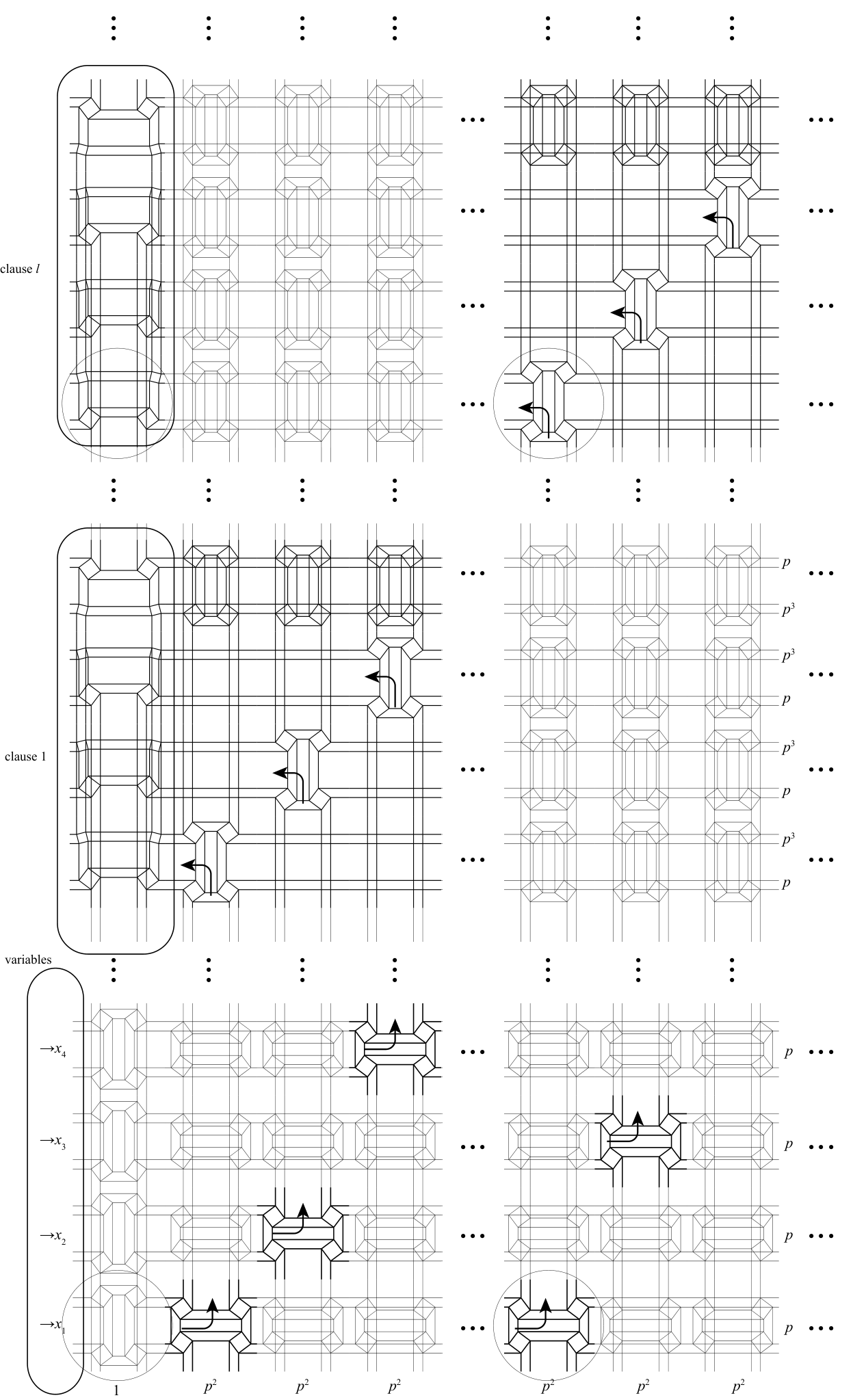

To prove this, we reduce from 1-in-3 SAT. Figure 6 shows the crease pattern for such a 1-in-3 SAT reduction, i.e., the crease pattern is rigidly foldable if and only if there is a set of binary variables that satisfy a given 1-in-3 SAT problem. The basic idea is that we describe binary variables by whether creases are folded (true) or not (false). This binary information will be carried via sets of four parallel creases, which we call wires. As we detail later, we carefully design gadgets, i.e., crease patterns connected to wires that are designed to be rigidly foldable for a given binary pattern of wires.
To overview the functional connection between gadgets, Figure 7 shows the schematic for designing such a crease pattern. The gadgets are designed to have two inputs of horizontal (from the left) and vertical (from below) wires, or multiple inputs from different horizontal wires from the right (in the case of the 1-in-3 clause gadgets), so that the wires carry their signals through the gadgets. Specifically, we design a splitter gadget (Figure 9) that copies a horizontal value to a vertical value and vice versa, a suppressor gadget (Figure 10) that enables a NAND operation between horizontal and vertical values, and a 1-in-3 clause gadget (Figure 11) that rigidly folds if and only if exactly one of three horizontal inputs are true. In addition, there are many intersections of horizontal and vertical wires. We carefully design our crease pattern so that these intersections merely cross over and do not logically interfere with one another. The gadgets are arranged in the crease pattern as follows (more detail is given in Section 4.2):
- 1.
The bottom horizontal wires represent the input variables . They are copied to vertical lines by using splitters and carried to each clause that uses this variable.
- 2.
Each set of four horizontal wires above the input variables section correspond to a clause. The copied variables in vertical lines are reflected horizontally using a grid of gadgets composed of splitters and suppressors. This forces that at most of variables to be true, and the folding of 1-in-3 clause gadget (thus making the clause be true) will ensure that exactly one of the horizontal wires must be true.
To prove that this works, we follow the following strategy. For each gadget, (1) we show that it successfully constrains the binary operations, i.e., it keeps wrong patterns from folding (the only if part), and (2) we give one MV assignment and rigid folding mode for each possible case of true and false (the if part). The first part will make sure that only if -SAT is solved, the pattern is rigidly foldable. The second part shows that there exists at least one possible assignment that makes the whole thing rigidly foldable.
4.1 The Gadgets
4.1.1 Wires
We extract a set of four parallel lines from the tessellation structure, and call them true if any of the four creases are folded, and false if none of the four creases are folding.
For true values we will use rigid folding modes of wires, which we call gutter and staircase, respectively (Figure 8). Note that the folding speeds measured in tangents of half the fold angles are different between two pairs of creases for a staircase wire. In our construction we will use a folding speed of , and the relative speed of the pairs of creases in a staircase will be .
4.1.2 Splitters

A splitter is the twist fold tessellation with a twist angle of , where the left and right horizontal wires are the input and the top and bottom vertical wires are the output (or the other way around) (Figure 9 left two). Note that we may think of both the left and right wires to be inputs (and both top and bottom to be outputs) because signals will always be unchanged as they travel through the splitter, either horizontally or vertically. A standard splitter will have all of its wires be gutters. A staircase splitter is a rotation of splitter, but its wires will have different modes so that the horizontal wire is a staircase and the vertical wire is a gutter. A widening splitter uses a pattern with two pairs of twists with angles (at the bottom) and (at the top) to change the widths of vertical wires. The folding mode of a widening splitter is designed to match with staircase horizontal wires and gutter vertical wires.
In what follows we denote the binary values of our gadgets with the notation where is the boolean value of the horizontal wires and is the value of the vertical wires.
Lemma 17.
A splitter, staircase splitter and widening splitter can fold only if they copy the values in the input to the output, and thus the possible patterns are (true, true) or (false, false).
Proof.
All horizontal creases are connected to vertical creases via degree- vertices with finite value of speed coefficients. If any of these creases fold, then every fold line in the gadget must fold, forcing the input and the output wires to have the same value. ∎
Lemma 18.
A splitter, staircase splitter and widening splitter can rigidly fold in the mode specified in Figure 9, where the numbers () assigned to the fold lines are the absolute relative folding speeds measured in tangent of half the fold angles.
Proof.
All splitters are composed of rigid origami twists as seen in Lemma 14. By consecutively mirroring the square twist in mode (a) of Figure 3 across horizontal and vertical axes, we obtain a splitter with the folding mode described in Figure 9. Because , the folding follows the specified speed.
The staircase splitter is obtained by rotating the normal splitter, but then changing some of the modes of the vertices (refer to Figure 2) so as to cascade the relative folding speed as shown in Figure 9. A widening splitter connects mode (a) of the square twist from Figure 3 with another square twist with a different twist angle. The consistent folding mode is ensured by having the bottom and top twists connected through folds with the same absolute speed and then having them mirrored with respect to the vertical line. Now, because we chose for the top twists, the top two creases folds times the speed of the bottom two creases. ∎
Remark 19.
Note that vertical wires are all gutters. Also, for the normal splitter, the speed of vertical wire is times the speed of horizontal wire. Moreover, the speed of the vertical wire in the staircase splitter is times that of widening splitter (when we synchronize the horizontal staircase wires of staircase and widening splitters).
4.1.3 Suppressor and Crossover Gadgets
Just overlaying two orthogonal wires (Figure 10 left) would make vertical and horizontal wires suppress each other so that they cannot be folded at the same time. We call this a suppressor, which only allows the patterns (false, false), (true, false), and (false, true).
Lemma 20.
A suppressor leaves all four horizontal creases unfolded or all four vertical creases unfolded.
Proof.
Any horizontal crease crosses perpendicularly to all vertical creases, forming degree- vertex with sector angles. Because the speed coefficients are at such a point, vertical creases cannot fold if horizontal crease have fold angle . ∎
This implies that we need to devise a crossover system to avoid logical interactions between horizontal and vertical wires.
A crossover gadget (Figure 10, right) is realized by overlaying the crease pattern of a splitter on top of a suppressor, where we line up the horizontal and vertical inputs. The overlaying of patterns allows us to chose either pattern to be active, so we get the union of the folding modes of splitters and suppressor, which complete four possible binary patterns.
Lemma 21.
Crossover gadgets can fold into four patterns (false, false), (true, false), (false, true) and (true, true). The folding modes of (true, false) and (false, true) patterns follow those of the corresponding wires, and the folding mode of (true, true) pattern follows that of a splitter.

4.1.4 Clause Gadget

A clause gadget is designed by overlaying three widening splitters in vertical direction, connected by one upside-down widening splitter on top (see Figure 11). We consider three bottom horizontal wires to be the literals, and the vertical wire gives the satisfiability. The fourth (top) horizontal wire, which is connected to the upside-down widening splitter, exists only for readjustment of widths to connect to the next clause on top.
Lemma 22.
A clause gadget folds only if exactly one of three inputs is true.
Proof.
Assume that the second input wire (from the bottom) is true. Because every horizontal crease in a clause gadget stops when it encounters a twist fold, all the twists must be folded in the second wire section. The vertical wires above the twists are wide, and the vertical wires bellow the twists are narrow. Therefore the twists connected to the first and third input wires will be suppressed, and the clause must form a (false, true, false) pattern. This is the same for the first and third horizontal wires, so we obtain (true, false, false) or (false, false, true) patterns. Because the bottommost vertical wire is narrow and the topmost vertical wire is wide, the vertical wire is foldable only if it uses at least one of the twists, but doing so will force us to chose one of three modes we have described. ∎
Lemma 23.
Clause gadget can fold in modes specified in Figure 11, which follows the folding mode of widening splitter and its upside down mirror image.
Proof.
The rigid folding motion follows that of widening splitter, and because the connected upside down splitter is compatible, they fold rigidly with the specified relative speed (in tangent half fold angle parameterization) in Figure 11. ∎
4.2 The proof (Layout)
Proof of Theorem 16.
For a given 1-in-3 SAT conjunctive normal form with clauses of variables , we construct a grid of horizontal wires and vertical wires , where we place a gadget at each intersection node of wires or at groups of nodes as specified bellow. By default, crossover gadgets are placed at unspecified nodes between horizontal and vertical wires.
We set the horizontal wires from to be the variables , and each set of four horizontal wires to be the th clause (). Specifically, for , we place a clause gadget at the intersection between and . The input variables of the clause are copied from , respectively; and the values of are copied from , respectively, by placing splitters at appropriate the intersections. We claim that the value of each of the vertical wires is constrained only by the 1-in-3 clause gadgets that they are attached to via splitters. This is because each of these vertical wires, if folding in a true signal, will (1) suppress the other vertical wires being fed into this clause and (2) cross other horizontal wires at a crossover gadget which will not change its value. By Lemmas 17, 20, 21 and 22, each clause can rigidly fold only if the clause returns true.
Now, because we concatenate all cause gadgets along , all clauses must be true if any clause is true. We claim that at least one clause must be true if any fold line is folded, therefore the whole laid out pattern can fold only if the given 1-in-3 SAT is satisfied. The claim follows because if all the clauses are false, then all variables are false and thus all horizontal wires are false. Because all vertical wires are the copies of variables, all vertical wires are also false, and thus the paper remains unfolded.
If 1-in-3 SAT is satisfied, we may assign true and false to each wire as appropriate. For wires with false, we can assume that they are removed from the crease pattern, which will result in a flat-foldable quadrivalent mesh composed of splitters, staircase splitters, widening splitters. For these creases, we assign the specified folding modes in Lemmas 18 and 23, so that they are compatible through the gutter and staircase wires at correct speeds. In particular, the synchronization between widening splitters and the staircase splitters is realized by the different speed between (with speed ) and (with speed ) as in Remark 19. To allow for a correct synchronization, we place rotated crossovers at the intersections between and so that the speed of the horizontal wire is times the speed of the vertical wire (Figure 12). More precisely, consider that the th clause’s th variable () is true, then each cycle formed by (1) the splitter at , (2) the staircase splitter at , (3) the widening splitter at as a part of clause gadget, and (4) the rotated splitter at as a part of crossover gadget rigidly folds with synchronized speeds at the creases. ∎

5 Conclusion
We have shown that judging rigid foldability of a crease pattern using all creases is weakly NP-hard (Theorem 15) and rigid foldability with optional creases is NP-hard (Theorem 16). The lower bound is not proven to be tight, as we do not know if this problem belongs to NP in general. As rigid origami is a special case of linkages, the rigid foldability problem belongs to Class [2]. We would like to know a tight lower bound in the future studies. For example, for flat-foldable degree--vertex origami, rigid foldability with given assignment is solvable in linear time, and thus rigid foldability belongs to NP (Theorem 13). Note that our work only proves weakly NP hardness of the model using all creases since the all-crease model does not allow for the overlay scheme for creating useful gadgets. It is still open if the hardness of two models differ.
Acknowledgements
This work was begun at the 2015 Bellairs Workshop on Computational Geometry, co-organized by Erik Demaine and Godfried Toussaint. We thank the other participants of the workshop for stimulating discussions.
References
- [1] Z. Abel, J. Cantarella, E. Demaine, D. Eppstein, T. Hull, J. Ku, R. Lang, and T. Tachi. Rigid origami vertices: conditions and forcing sets. Journal of Computational Geometry, 7(1):171–184, 2016.
- [2] Zachary Abel, Erik D. Demaine, Martin L. Demaine, Sarah Eisenstat, Jayson Lynch, and Tao B. Schardl. Who needs crossings? hardness of plane graph rigidity. In 32nd International Symposium on Computational Geometry, SoCG 2016, June 14-18, 2016, Boston, MA, USA, pages 3:1–3:15, 2016.
- [3] Hugo A. Akitaya, Kenneth C. Cheung, Erik D. Demaine, Takashi Horiyama, Thomas C. Hull, Jason S. Ku, Tomohiro Tachi, and Ryuhei Uehara. Box pleating is hard. In Discrete and Computational Geometry and Graphs: 18th Japan Conference, JCDCGG 2015, Kyoto, Japan, September 14-16, 2015, Revised Selected Papers, pages 167–179, Cham, 2016. Springer International Publishing.
- [4] alex.jordan. Rapid approximation of . Mathematics Stack Exchange, February 2012. https://math.stackexchange.com/q/107309.
- [5] s.-m. belcastro and T. Hull. Modelling the folding of paper into three dimensions using affine transformations. Linear Algebra and its Applications, 348:273–282, 2002.
- [6] Marshall Bern and Barry Hayes. The complexity of flat origami. In Proc. 7th ACM-SIAM Symposium on Discrete Algorithms (SODA ’96), pages 175–183, 1996.
- [7] R. Bricard. Mémoire sur la théorie de l’octaèdre articulé. J. Math. Pures Appl., 3:113–150, 1897.
- [8] Christoph Burnikel, Stefan Funke, Kurt Mehlhorn, Stefan Schirra, and Susanne Schmitt. A separation bound for real algebraic expressions. Algorithmica, 55(1):14–28, September 2009.
- [9] C. H. Chiang. Kinematics of Spherical Mechanisms, 2nd ed. Krieger Publishing Co., Malabar, FL, 2000.
- [10] Jian S. Dai. Configuration transformation and mathematical description of manipulation of origami cartons. In K. Miura, T. Kawasaki, T. Tachi, R. Uehara, R. J. Lang, and P. Wang-Iverson, editors, Origami6, pages 163–173. The American Mathematical Society, 2015.
- [11] E. D. Demaine and J. O’Rourke. Geometric Folding Algorithms: Linkages, Origami, Polyhedra. Cambridge University Press, Cambridge, 2007.
- [12] T. A. Evans, R. J. Lang, S. P. Magleby, and L. L. Howell. Rigidly foldable origami twists. In K. Miura, T. Kawasaki, T. Tachi, R. Uehara, R. J. Lang, and P. Wang-Iverson, editors, Origami6, pages 119–130. The American Mathematical Society, 2015.
- [13] S. Fujimoto and M. Nishikawa. Seizo suru origami asobi no shotai (Creative Invitation to Playing with Origami, in Japanese). Asahi Culture Center, Tokyo, 1982.
- [14] D. A. Huffman. Curvature and creases: A primer on paper. IEEE Transactions on Computers, 25(10):1010–1019, 1976.
- [15] T. Hull. Counting mountain-valley assignments for flat folds. Ars Combinatoria, 67:175–187, 2003.
- [16] T. Hull. Project Origami: Activities for Exploring Mathematics, 2nd ed. A K Peters/CRC Press, Wellesley, MA, 2012.
- [17] S. A. Robertson. Isometric folding of Riemannian manifolds. Proc. of the Royal Society of Edinburgh, 79(3-4):275–284, 1977.
- [18] M. Schenk, S. G. Kerr, A. M. Smyth, and S. D. Guest. Inflatable cylinders for deployable space structures. In F. Escrig and J. Sánchez, editors, Proc. of the First Conference Transformables 2013, In the Honor of Emilio Pérez Piñero, Seville, Spain, Madrid, Spain, 2013. Starbook Editorial.
- [19] J. L. Silverberg, A. A. Evans, L. McLeod, R. Hayward, T. Hull, C. D. Santangelo, and I. Cohen. Using origami design principles to fold reprogrammable mechanical metamaterials. Science, 345(6197):647–650, 2014.
- [20] T. Tachi. Rigid-foldable thick origami. In P. Wang-Iverson, R. J. Lang, and M. Yim, editors, Origami5: Fifth Int. Meeting of Origami Science, Mathematics, and Education, pages 253–263, Boca Raton, FL, 2011. CRC Press.
- [21] Tomohiro Tachi. Freeform rigid-foldable structure using bidirectionally flat-foldable planar quadrilateral mesh. In Cristiano Ceccato, Lars Hesselgren, Mark Pauly, Helmut Pottmann, and Johannes Wallner, editors, Advances in Architectural Geometry 2010, pages 87–102. Springer Vienna, 2010.
- [22] Tomohiro Tachi and Thomas C. Hull. Self-foldability of rigid origami. Journal of Mechanisms and Robotics, 9(2):021008–021017, 2016.