A Nonlinear Transform for the Diagonalization of the Bernoulli-Laplace Diffusion Model and Orthogonal Polynomials

The Bernoulli-Laplace (BL) model arise from diffusion theory and is related to the shuffling of cards [8]. Symmetries of the permutation group $S_{N}$ appear naturally in this model and other random walks on groups. Previous solutions of this model have appeared in Diaconis and Shashahani [7] and in the works of Karlin and MacGregor [10]. Group representations are used explicitly in the first; the derivation of a non-standard inner product or equivalently a measure for orthogonal polynomials which are related to the eigensolutions of the BL model appears in the second.

In this paper, we give a third way for deriving exact solutions of all the eigenvectors of the BL model, through a nonlinear transform that triangularizes and then diagonalizes the transition matrix $T_{BL}$. In brief, our method associates a specific linear partial differential operator (LPDO) $L_{BL}$ that acts on the vector space of homogeneous polynomials, $G,$ to the matrix $T_{BL}$. The $L_{BL}$ inherits the symmetries of the BL model; it encodes the tri-diagonal singly-stochastic (column sums are equal to 1 ) and anti-symmetric structure of $T_{BL}$. The components of the (right) eigenvectors (in view of the equal column sums of $T_{BL})$ of $T_{BL}$ is encoded in the coefficients of the homogeneous polynomial $G.$ A classical theory for the symmetries of such LPDOs have been formulated in terms of the Lie algebra of symmetry operators $K$ that commutes with $L_{BL}$ (cf. [13]).

It turns out and we exploit in our method, that the symmetries of $L_{BL}$ appear iu the form of suitable linear and nonlinear transformations $P$ on the independent variables $x,y,$ etc. or indeterminates of $G.$ The ease of use of this method resides in the transparent or explicit way to find these transformations $P.$ Our algorithm is completed by associating the transformed LPDO, $L_{BL}^{\prime},$back to what turns out to be a triangular matrix $T_{BL}^{\prime}$; in other words, the transformation $P$ for $L_{BL}$ encodes a similarity transformation that triangularizes $T_{BL},$ i.e., $PT_{BL}P^{-1}=T_{BL}^{\prime}$, which is then solved directly for its eigenvalues and right eigenvectors.

Here, we give a summary of the Urn models to which the BL model is related as an extension. The Ehrenfest model and the Polya Urn models are two of the early solvable models in the literature [9]. They appear as two of the exactly solved cases in Friedman’s formulation of Urn models where precisely one urn and balls of two colors are drawn and replaced with additions [9]. A dual formulation of Friedman’s Urn models was introduced in a series of recent papers [16, 14]: instead of balls of two colors and one urn, the dual formulation uses two urns and one-colored balls. The latter is more convenient for modelling of certain network science models [3], such as the Voter model where two balls are drawn and returned to the two urns with prescribed probabilities that depend on the order in which they are drawn. This is because many of the network science models are irreversible Markov chain models [4] which have absorbing states. Their transition matrices $T$, unlike $T_{BL}$ for the BL model, are not symmetric, in an essential sense, that is, there are no non-standard inner products for $R^{N}$ in which these matrices $T$ have a symmetric form.

Using a new method based on diagonalization of transition matrices [15], we solved exactly the eigenvectors of several well-known models, including the Ehrenfest model, the Voter model [18, 12, 11, 5, 17, 2], the Moran model for genetic drift, and the Naming game models [19], [20]. Most of these models are irreversible Markov models with absorbing states, and have essentially non-symmetric transition matrices in the sense just mentioned. The BL model however, is based on two urns and balls of two colors. Thus, it is not strictly in the class of Two Urns models to which we recently applied our method. In modifying this method so that it applies to the BL model, we will have shown that the new method is not only easy to use but also flexible in extension to new problems.

One of the main points here is the technical simplicity of uncovering the symmetries of the above LPDOs within our method, through the explicit appearance of the expressions $u=f(x,y)$ in the coefficients of $L.$ We give here the LPDO $L_{V}$ for the Voter model [16, 14] to indicate what we mean: first the propagation equation for the transition matrix $T_{V}$ is given by

	$\displaystyle a_{j}^{(m+1)}$	$\displaystyle=$	$\displaystyle p_{j-1}a_{j-1}^{(m)}+(1-2p_{j})a_{j}^{(m)}+p_{j+1}a_{j+1}^{(m)}$		(1)
	$\displaystyle p_{j}$	$\displaystyle=$	$\displaystyle\frac{j(N-j)}{N(N-1)};$		(2)

the eigen-problem for the associated LPDO $L_{V}$ $=(x-y)^{2}G_{xy}$ acting on the homogeneous polynomial $G(x,y)=\sum_{j}c_{j}x^{j}y^{N-j}$ (which encodes the components $c_{j}$ of the right-eigenvector of $T_{V})$ is given

$$(x-y)^{2}G_{xy}=N(N-1)(\lambda-1)G,$$

(3)

which clearly suggests the transformation $u=x-y,$ $v=y.$ Indeed this triangularized and diagonalized the Voter model and led to its complete solution.

Contrast this ease of use with the fact that triangularization and diagonalization of a given transition matrix of size $N$ has computational complexity $O(N^{3}).$ In other words, exact integration of the Two Urns models via diagonalization of transition matrices are nontrivial problems, that are difficult to solve but once known, the solutions are easy to verify. [16, 14] provides a simple method to find such explicit diagonalization and hence all eigenvectors for a class of transition matrices from the Two Urns models, even when their transition matrices are essentially non-symmetric. Note that the eigenproblem and diagonalization of symmetric matrices have a lower computational complexity.

We aim here to highlight this method’s ease of use, relative to the group representation method and the method of orthogonal polynomials. Moreover, the BL model differs significantly from the original Two Urns subclass of models for which our method was initially formulated. Thus, we also aim to show that, with the specific introduction of a nonlinear change of independent variables, this method can be applied to more complex models than the original class of models. Since the BL transition matrix $T_{BL}$ is from a reversible Markov chain with a stationary distribution [4], it is non-symmetric singly-stochastic only in a trivial sense. In other words, there exists (a difficult to find) non-standard inner product for $R^{N},$ in which $T_{BL}$ is symmetric and hence doubly-stochastic. Karlin and McGregor [10] using their powerful integral representation method of finding an explicit way to symmetrize $T$ by introducing a non-standard inner product (or orthogonal measure) into the problem, have related the right eigenvectors of the transition matrix $T_{BL}$ of the $BL$ model to the orthogonal polynomials called the dual Hahn polynomials. A third aim of this paper is therefore to re-derive from the diagonalization of $T_{BL},$ this non-standard inner product in which the dual Hahn polynomials are an orthogonal polynomial system. Note that this non-standard inner product, once found, yields a symmetric version of $T_{BL}$which is an example of a Jacobi operator that arise in the the classical moments problem [1], and is related to orthogonal polynomials via the Riemann-Hilbert method [6].

The paper is organized as follows: section 3 concerns the calculation of the right eigenvectors and eigenvalues of $T$ in closed form by method introduced in [16, 15, 14]; in view of the fact that these right eigenvectors are not orthogonal in the usual Euclidean inner-product, section 4 concerns the transformations needed to calculate the orthonormal system of left eigenvectors of $T_{BL},$and also the derivation of the non-standard inner product in which the right eigenvectors are now orthogonal; section 5 concerns the elementary proofs, based only on the eigenvectors and eigenvalues of $T,$ for the tight upper and lower bounds for times to stationarity in the BL model [7] ; section 6 concerns a numerically exact evaluation of the expression for the TV norm in these bounds using the eigenvectors and eigenvalues of $T_{BL}$ directly, hence slightly sharper estimates for the mixing times of the BL model.

Beyond the balanced special case of the BL problem treated in detail in this paper, the same generating function method can be used to prove similar tight bounds for mixing times in the other cases.

Let the transition matrix $T_{BL}$ be defined so that $(T_{BL\text{ }})_{ij}=Pr\{n_{w}(m+1)=i\;|\;n_{w}(m)=j\}$, so that the sum of each column is $1$. In the general BL model for balls of two colors and two urns, $N_{1},$ $N_{2},$ $N_{w},$ $N_{b}$ are fixed parameters satisfying the constraints

$$N_{w}+N_{b}=N=N_{1}+N_{2}$$

(4)

where $N$ equals total number of balls in the model. For $i=0,...,N_{w}\leq N_{1},$ (where by abuse of notation $i$ stands for both the row label of transposed matrix $T_{BL}^{t}$ and the number of white balls in urn 1, $n_{w}),$ the transition probabilities are explicitly given by

	$\displaystyle p_{i}$	$\displaystyle=$	$\displaystyle\Pr\left\{n_{w}(t+1)=i+1|\text{ }n_{w}(t)=i\right\}=\frac{\left(N_{1}-i\right)\left(N_{w}-i\right)}{N_{1}N_{2}}$		(5)
	$\displaystyle q_{i}$	$\displaystyle=$	$\displaystyle\Pr\left\{n_{w}(t+1)=i-1|\text{ }n_{w}(t)=i\right\}=\frac{i\left(N_{b}-\left(N_{1}-i\right)\right)}{N_{1}N_{2}}$		(6)
	$\displaystyle r_{i}$	$\displaystyle=$	$\displaystyle\Pr\left\{n_{w}(t+1)=i|\text{ }n_{w}(t)=i\right\}=1-q_{i}-p_{i}.$		(7)

.

In [16, 14], we developed an explicit method for exactly integrating or solving a 5-parameters subclass of a class of Two Urns models which is parametrized by six real parameters. Our method is based on a relationship between certain banded stochastic matrices $T$ (such as tridiagonal and pentadiagonal non-symmetric transition matrices of markov chain models) and the LPDOs acting on the vector space of homogeneous polynomials, $G(x,y)$ of finite order in two indeterminates. The symmetries of the LPDO, $L,$ associated with a given non-symmetric singly stochastic matrix from this solvable subclass of the Two Urns models, are identified and used explicitly to transform from the original indeterminates ( independent variables $x,y$ say) to suitable new variables (such as $u=f(x,y),v=g(x,y)$). In the new variables $u,v,$ the transformed LPDO, $L^{\prime},$ acts on the (again homogeneous of same order as $G(x,y))$ polynomial $H(u,v).$ We have shown in [16, 14] that the transformed eigen-problem

$$L^{\prime}[H(u,v)]=\lambda(N)H(u,v)$$

(8)

for a well-defined subclass of such Two Urns problems is equivalent (via the inverse of the original relationship between banded matrix and LPDO) to the eigen-problem for a triangular matrix, which can then be solved explicitly for both right and left eigenvectors. In other words, at the end of this brief summary, the symmetries of LPDO $L$ inherited from the original banded stochastic matrix $T,$generate an explicit similarity transformation, $P,$ such that

$$STS^{-1}=D$$

(9)

where $D$ is diagonal, and $S$ contains the eigenvectors of $T.$

This method can be formalized as an Algorithm as follows: Given the input of a singly stochastic transition matrix $T$ of size $N+1$,

(I) Choose a suitable homogeneous polynomial of finite degree $N$, $G$ that has the components $c_{i}$ of a right eigenvector of $T$ as coefficients of the monomials $x^{i}y^{j}z^{k}$; part of this choice is the number of indeterminates in $G$. For example, the Voter model of size N (number of balls) with a transition matrix $T_{V}(N)$ which is a $N+1$ by $N+1$ real matrix, requires a homogeneous polynomial $G_{V}$ of degree $N$ in the indeterminates $x,y$ because there are two urns.

(II) Associate the recursion inplicit in given Markov matrix $T$ to a LPDO, $L$ which acts on the homogeneous polynomial $G$; the basic elements of this association scheme are the standard linear differential operators for increasing, decreasing and not changing the numbers of balls in each urn (which correspond in the example below to the probabilities $p,q,r$ prescibed by the transition matrix), and a set of multiplication type linear operators that correspond to shifts.

(III) A transformation to new independent variables,(for instance, $u=f(x,y,z),$ $v=g(x,y,z),$ $w=h(x,y,z)$) is chosen to satisfy two conditions:

$(A)$ the transformed polynomial

$$H(u,v,w)=H(f(x,y,z),g(x,y,z),h(x,y,z))=G(x,y,z)$$

is a homogeneous polynomial of the same finite degree as $G;$

$(B)$ $u=f(x,y,z),$ $v=g(x,y,z),$ $w=h(x,y,z)$ is a transformation based on the symmetries of $L$ (cf. [13]), that is, the combinations $f(x,y,z),$ $g(x,y,z),$ $h(x,y,z)$ of the original variables $x,y,z$ appear naturally in the coefficients of the LPDO, $L.$

These conditions $(A)$ and $(B)$ are clearly not sufficient to ensure the transformed LPDO eigenproblem

$$L^{\prime}[H(u,v,w)]=\lambda(N)H(u,v,w)$$

(10)

is associated with a similar triangular matrix $T^{\prime}$ which explicitly yields all its eigenvectors $b_{i}$. That they are sufficient has to be proved either in each problem to which we apply the Algorithm, or for a class of models as in the case of the Two Urns models.

(IV) Using the transformation in step (III), derive the corresponding transformed LPDO, $L^{\prime}$ that acts on the transformed polynomial $H(u,v,w)$.

(V) Without explicitly calculating the transformed matrix $T^{\prime}$ which is associated with the transformed LPDO, $L^{\prime}$ in step (IV), check that the transformed eigen-problem for $L^{\prime}$ is indeed a recursion system for the transformed eigenvectors $b_{i}$ that can be solved explicitly, i.e., it is equivalent to a triangular linear system of equations. Solve for the eigenvalues and then the eigenvector components $b_{i}$, and if required transform back to the original components $c_{i}$. These are the main outputs of the Algorithm.

(VI) Use the eigenvectors in step (V) to diagonalize the original matrix if necessary. This is the end of the ALgorithm.

Now we apply the Algorithm to the BL model. Given the transition matrix of the BL model (cf. section 2), it will be obvious that three independent variables (instead of the two before) should be used to formulate the BL problem. In step (I) of the Algorithm, we adopt the anzatz that the $LPDO,$ $L_{BL},$ associated with the above $N$ by $N$ matrix $T_{BL}$, now acts on a homogeneous polynomial $G(x,y,z)$ in three indeterminates, $x,y,z.$ We encode the entries $c_{k}(i)$, $i=0,...,N_{w}$ of the $k-th$ eigenvector of the transition matrix for the BL model as follows:

$$G^{(k)}(x,y,z)=\sum_{i=0}^{N_{w}}c_{k}(i)x^{i}y^{N_{1}-i}z^{N_{w}-i}.$$

(11)

where $i=$ number of white balls in urn 1 (also denoted $n_{w})$. The choice of three independent variables to encode the components of an eigenvector of $T_{BL}$ in the homogeneous polynomial $G(x,y,x)$ is now made obvious by this explicit expression for $G.$

In step (II) of the Algorithm, we derive from the original eigen-problem for transition matrix $T_{BL},$ an LPDO, $L_{BL}$, that acts on $G^{(k)}$. Towards that aim, we note, in particular, the entries for $p_{i}$ and $q_{i}$ in $T_{BL}$ correspond respectively to the following linear differential operators with coefficients that are monomials in $x,y,$and $z,$

	$\displaystyle L_{p}=$		$\displaystyle\frac{yzG_{yz}^{(k)}}{N_{1}N_{2}}$		(12)
	$\displaystyle L_{q}=$		$\displaystyle\frac{N_{b}x}{N_{1}N_{2}}G_{x}^{(k)}-\frac{xy}{N_{1}N_{2}}G_{xy}^{(k)},$		(13)

where $G_{yz}^{(k)}=\frac{\partial^{2}}{\partial y\partial z}G^{(k)}$ for example. In addition, it is part of the association scheme that multiplication in the LPDO (cf. [13]) by the coefficient $\frac{x}{yz}$ (resp. $\frac{yz}{x})$ represents down (resp. up) shifts in the index $i$ within the discrete recursion equations of the original eigen-problem for matrix $T_{BL.}$ The $L_{BL}$ associated with the eigen-problem of the tridiagonal Markov matrix $T_{BL}$is given by:

	$\displaystyle L_{BL}[G^{(k)}]$	$\displaystyle=$	$\displaystyle N_{1}N_{2}\left(\lambda_{k}-1\right)G^{(k)}$		(14)
	$\displaystyle L_{BL}[G^{(k)}]$	$\displaystyle\equiv$	$\displaystyle\left(x-yz\right)G_{yz}^{(k)}+y\left(x-yz\right)G_{xy}^{(k)}-N_{b}\left(x-yz\right)G_{x}^{(k)}.$		(15)

In step(III) of the Algorithm, we note that the symmetries of $L_{BL}$ with respect to transformations of its independent variables, is expressed in the factor $\left(x-yz\right)$ in its coefficients. This suggests the transformation to the new independent variables

$$u=x-yz,y=y,z=z.$$

(16)

Since the transformed homogeneous polynomial is now given by

$$H^{(k)}(u,y,z)=G^{(k)}(x(u,yz),y,z)=\sum_{i}b_{i}^{k}u^{i}y^{N_{1}-i}z^{N_{w}-i}$$

(17)

in terms of the (new) components $b_{i}^{k}$ of the $k-th$ right eigenvector, this transformation clearly satisfies both necessary conditions (A) and (B) in step (III) of the Algorithm.

To prove that it is sufficient for our purpose of obtaining the eigenvalues and eigenvectors exactly and for diagonalization, we proceed by direct calculations.

In step (IV) using the following obvious identities for the transformation of partial derivatives

	$\displaystyle\partial_{x}$	$\displaystyle=$	$\displaystyle\partial_{u}$		(18)
	$\displaystyle\partial_{y}$	$\displaystyle=$	$\displaystyle\partial_{y}-z\partial_{u}$		(19)
	$\displaystyle\partial_{z}$	$\displaystyle=$	$\displaystyle\partial_{z}-y\partial_{u}$		(20)
	$\displaystyle\partial_{xy}$	$\displaystyle=$	$\displaystyle\partial_{yu}-z\partial_{u}^{2}$		(21)
	$\displaystyle\partial_{yz}$	$\displaystyle=$	$\displaystyle\partial_{yz}-y\partial_{yu}-z\partial_{uz}+yz\partial_{u}^{2}-\partial_{u}$		(22)

the transformed LPDO, $L_{BL}^{\prime}$ in $H^{(k)}$, $k=0,...,$ $N_{w}$ is

	$\displaystyle N_{1}N_{2}(\lambda_{k}-1)H^{(k)}$	$\displaystyle=$	$\displaystyle L_{BL}^{\prime}[H^{(k)}],$		(23)
	$\displaystyle L_{BL}^{\prime}[H^{(k)}]$	$\displaystyle=$	$\displaystyle-N_{b}u\partial_{u}H^{(k)}+yu\left(\partial_{yu}-z\partial_{u}^{2}\right)H^{(k)}$		(25)
			$\displaystyle+u\left(\partial_{yz}-y\partial_{yu}-z\partial_{uz}+yz\partial_{u}^{2}-\partial_{u}\right)H^{(k)}$
		$\displaystyle=$	$\displaystyle u\left(\partial_{yz}-z\partial_{uz}\right)H^{(k)}-(N_{b}+1)u\partial_{u}H^{(k)}$		(26)

In step (V), by reversing the derivation of the original $L_{BL}$ through the association scheme [13], this $L_{BL}^{\prime}$ in $H$ is shown to be equivalent to the following triangular system for the (right) eigen-problem of the transformed matrix $T_{BL}^{\prime}$:

			$\displaystyle N_{1}N_{2}(\lambda_{k}-1)b_{i}^{k}$		(27)
		$\displaystyle=$	$\displaystyle\left(N_{1}-i+1\right)\left(N_{w}-i+1\right)b_{i-1}^{k}-i\left(N_{w}-i\right)b_{i}^{k}-(N_{b}+1)ib_{i}^{k}.$		(28)

We have therefore verified the sufficiency of the transformation where $u=x-yz$ for triangularizing (and later diagonalizing) $T_{BL}.$ This triangular system implies the recursion

$$b_{i}^{k}=\frac{\left(N_{1}-i+1\right)\left(N_{w}-i+1\right)b_{i-1}^{k}}{N_{1}N_{2}(\lambda_{k}-1)+i\left(N_{w}-i\right)+(N_{b}+1)i}$$

(29)

which can be solved directly.

For nontrivial eigensolutions for $k=0,...,N_{w},$ the denominator in $b_{i}^{k}$ must vanish, yielding the following exact expressions for the eigenvalues,

	$\displaystyle\lambda_{k}$	$\displaystyle=$	$\displaystyle 1-\frac{k\left(1-k+N_{w}+N_{b}\right)}{N_{1}N_{2}}$		(30)
		$\displaystyle=$	$\displaystyle 1-\frac{k\left(1-k+N\right)}{N_{1}N_{2}}$		(31)
		$\displaystyle=$	$\displaystyle 1-\frac{k\left(N-k+1\right)}{N_{1}N_{2}}$		(32)

In the case $N_{1}=N_{w},$

	$\displaystyle\lambda_{0}$	$\displaystyle=$	$\displaystyle 1$		(33)
	$\displaystyle\lambda_{1}$	$\displaystyle=$	$\displaystyle 1-\frac{N}{N_{1}N_{2}}.$		(34)

The eigenvectors (in the transformed variables of $H)$ are given explicitly by:

	$\displaystyle b_{i}^{k}$	$\displaystyle=$	$\displaystyle\prod_{j=k+1}^{i}\frac{\left(N_{1}-j+1\right)\left(N_{w}-j+1\right)}{N_{1}N_{2}(\lambda_{k}-1)+j\left(N_{w}+N_{b}+1-j\right)}$		(35)
		$\displaystyle=$	$\displaystyle\prod_{j=k+1}^{i}\frac{\left(j-N_{1}-1\right)\left(j-N_{w}-1\right)}{-k\left(N+1-k\right)+j\left(N+1-j\right)}$		(36)
		$\displaystyle=$	$\displaystyle\prod_{j=k+1}^{i}-\frac{\left(j-N_{1}-1\right)\left(j-N_{w}-1\right)}{\left(j-k\right)\left(j+k-N-1\right)}$		(37)
		$\displaystyle=$	$\displaystyle(-1)^{i-k}\frac{(k-N_{1})_{i-k}(k-N_{w})_{i-k}}{(i-k)!(2k-N)_{i-k}}.$		(38)

Using these coefficients in the definition for $H$ gives

$$H^{(k)}=\sum_{i=k}^{N^{\prime}}(-1)^{i-k}\frac{(k-N_{1})_{i-k}(k-N_{w})_{i-k}}{(i-k)!(2k-N)_{i-k}}u^{i}y^{N_{1}-i}z^{N_{w}-i}$$

(39)

We summarize the consequences of the above steps of the Algorithm on the BL model in the following theorem:

For transition matrix $T_{BL},$ let $Z$ be given by (where we drop the subscript BL herein, i.e., $T=T_{BL}$)

$$Z_{ij}=\sqrt{\pi_{j}}T_{ij}\frac{1}{\sqrt{\pi_{i}}}.$$

(47)

Recall the detailed balance of $T$ and its stationary distribution, given by $T_{ij}\pi_{j}=T_{ji}\pi_{i}$ [4] follows from the reversibility and ergodicity of the BL model. Note that $Z$ is the symmetric version of the transition matrix:

	$\displaystyle Z_{ij}$	$\displaystyle=\frac{1}{\sqrt{\pi_{j}}}\pi_{j}T_{ij}\frac{1}{\sqrt{\pi_{i}}}$		(48)
		$\displaystyle=\frac{1}{\sqrt{\pi_{j}}}T_{ji}\sqrt{\pi_{i}}$		(49)
		$\displaystyle=Z_{ji}.$		(50)

Therefore, $Z$ has an orthonormal set of left eigenvectors, $w_{k}^{T}$. Let $W$ be a matrix whose columns are $w_{k}$. The spectral decomposition of $Z$ by left eigenvectors is given by

$$Z=W\Lambda W^{T}.$$

(51)

By the definition of $Z_{ij}$, the transformation from $T$ to $Z$ can be expressed as

$$D^{-1}TD=Z,$$

(52)

where $D$ is a diagonal matrix whose diagonal entries are $\sqrt{\pi_{i}}$. So, arbitrary powers of $T$ is given by

$$T^{m}=DW\Lambda^{m}(D^{-1}W)^{T}.$$

(53)

Defining a new transformation by $S,$

$$T^{m}=S\Lambda^{m}S^{-1}.$$

(54)

Since $W$ has a specific normalization, we can equate $S$ with $DW$ after applying the appropriate normalization for $S$. That is, for diagonal matrix $\Delta$, we take

$$S\Delta=DW.$$

(55)

We can choose any normalization for the right eigenvectors given in $S$, and $\Delta$ will properly renormalize them. Here, we solve for $\Delta$ and $W$ by appealing to the orthogonality of $W$:

$$W^{T}W=\Delta S^{T}D^{-2}S\Delta=I.$$

(56)

Therefore

$$S^{T}D^{-2}S=\Delta^{-2}.$$

(57)

Computing the matrix multiplication on the left side yields the diagonal entries of $\Delta$ denoted by $\Delta_{k}$ given by

$$\Delta_{k}^{-2}=\sum_{i=0}^{N}\frac{1}{\pi_{i}}c_{k}(i)^{2}$$

(58)

in terms of the right eigenvectors of $T_{BL}.$ Now that we have $\Delta$, we have the representations for both the left-eigenvectors $w_{k}(i)$ and right-eigenvectors $v_{k}(i)$ of $Z$ given by

	$\displaystyle w_{k}(i)$	$\displaystyle=\frac{\Delta_{k}}{\sqrt{\pi_{i}}}c_{k}(i)$		(59)
	$\displaystyle v_{k}(i)$	$\displaystyle=\frac{1}{\sqrt{\pi_{i}}}w_{k}(i)=\frac{\Delta_{k}}{\pi_{i}}c_{k}(i)$		(60)

in terms of the right-eigenvectors $c_{k}(i)$ of the original $T_{BL}$ that was obtained by our method in section 2.

From Eq. (57), we also have an explicit formula for $S^{-1}$ given by

$$S^{-1}=\Delta^{2}S^{T}D^{-2}.$$

(61)

So, by Eq. (54), we have

$$T^{m}=S\Lambda^{m}\Delta^{2}S^{T}D^{-2}.$$

(62)

Computing the matrix multiplication gives the following spectral decomposition

$$T_{ij}^{(m)}=\frac{1}{\pi_{j}}\sum_{k=0}^{N}\Delta_{k}^{2}\lambda_{k}^{m}c_{k}(i)c_{k}(j).$$

(63)

as the explicit representation of $Pr\{n(m)=i\;|\;n(0)=j\}$ in the BL model.

Since $T^{0}=I$, take $m=0$ in Eq. (63) to find the stationary distribution of the BL model

$$\pi_{j}\delta_{ij}=\sum_{k=0}^{N}\Delta_{k}^{2}c_{k}(i)c_{k}(j).$$

(64)

Note that this is the orthogonality relation for the right-eigenvectors of $T_{BL}$ with orthogonal measure $\Delta_{k}^{2}$ given in Eq. (63). We have derived the orthogonal measure $\Delta_{k}^{2}$ in which the dual Hahn are an orthogonal polynomial system [10].

We summarize these results on the derivation of a non-standard inner product or orthogonal measure in which the original transition matrix of the BL model becomes a symmetric real matrix and the (right) eigenvectors are the system of orthogonal dual Hahn polynomials:

We will discuss first the case $N_{1}=N_{2}=N/2,$ for our method gave the eigenvalues of the BL model to be $\lambda_{k}=1-\frac{4k\left(N-k+1\right)}{N^{2}},$ $\lambda_{1}=1-\frac{4}{N}.$ A heuristic estimate of the number of switches $q$ needed to mix the colors is thus,

$$(1-\frac{4}{N})^{q}\simeq e^{-\frac{4q}{N}}=\frac{1}{N},$$

(65)

and therefore $q=\frac{1}{4}N\log N$ gives an idea of how many switches or time steps are needed until the variation distance between $\rho_{q}$ and $\pi$ is of order $O(1/N).$ The lower bound is obtained along the lines of Diaconis et al, that is, by an application of the Chebyshev’s inequality. However, all estimates of the relevant mean values and variance needed to apply the Chebyshev’s inequality are constructed explicitly from the properties of the eigenvalues and eigenvectors of the BL model. We will state the theorems below but since the proofs are similar to those in [7], we have provided the details in an appendix.

Given that we can calculate $\rho_{m}(i,j)$ exactly by Eq. (63), and the stationary distribution is given by

$$\pi_{i}=\frac{{\binom{N_{w}}{i}}{\binom{{N-N_{w}}}{{N_{1}-i}}}}{{\binom{N}{N_{1}}}},$$

(66)

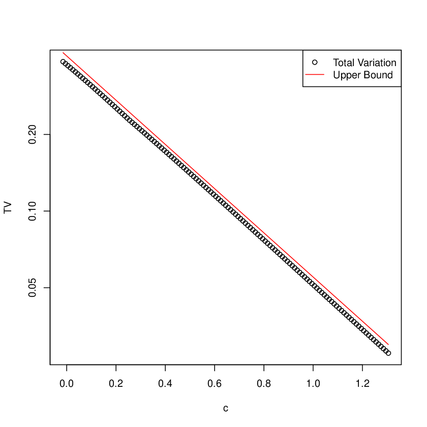
the total variational distance can be exactly computed for all time steps by

$$\|\rho-\pi\|_{V}=\frac{1}{2}\sum_{i=0}^{N/2}\left|\pi_{i}\sum_{k=1}^{N/2}\lambda_{k}^{m}v_{k}(i)v_{k}(0)\right|$$

(67)

This solution is shown in Figure 1, with the upper bound given in Figure 2.

References

- [1] N. Akhiezer, The Classical Moment Problem, Hafner, 1965.
- [2] A. Baronchelli, C. Castellano, and R. Pastor-Satorras, Voter models on weighted networks, Phys. Rev. E, 83 (2011), p. 066117.
- [3] A. Baronchelli, M. Felici, V. Loreto, E. Caglioti, and L. Steels, Sharp transition towards shared vocabularies in multi-agent systems, J. Stat. Mech.: Theory Exp., (2006), p. P06014, http://stacks.iop.org/1742-5468/2006/i=06/a=P06014.
- [4] P. Bremaud, Markov chain models, Springer-Verlag, 2005.
- [5] F. Caccioli, L. Dall’Asta, T. Galla, and T. Rogers, Voter models with conserved dynamics, Phys. Rev. E, 87 (2013), p. 052114.
- [6] P. Deift, Orthogonal Polynomials and Random Matrices, Courant Lecture Notes 3, 2000.
- [7] P. Diaconis and M. Shahshahani, Time to reach stationarity in the bernoulli–laplace diffusion model, SIAM Journal on Mathematical Analysis, 18 (1987), pp. 208–218.
- [8] L. Flatto, A. M. Odlyzko, and D. Wales, Random shuffles and group representations, The Annals of Probability, (1985), pp. 154–178.
- [9] B. Friedman, A simple urn model, CPAM, 2 (1949), pp. 59–70.
- [10] S. Karlin and J. McGregor, Random walks, Illinois J. Math., 3 (1959).
- [11] N. Masuda, Voter models with contrarian agents, Phys. Rev. E, 88 (2013), p. 052803.
- [12] N. Masuda, N. Gilbert, and S. Redner, Heterogeneous voter models, Phys. Rev. E, 82 (2010), p. 010103(R).
- [13] P. Olver, Equivalence, Invariants and Symmetries, North Holland, New York, 2005.
- [14] W. Pickering, Solution of Urn Models by Generating Functions with Applications to Social, Physical, Biological, and Network Sciences, PhD thesis, Dept. Math. Sci., Rensselaer Polytechnic Institute, Troy, NY, 2016.
- [15] W. Pickering and C. Lim, Solution to urn models of pairwise interaction with application to social, physical, and biological sciences, Phys. Rev. E, 96(1).
- [16] W. Pickering and C. Lim, Solution of the voter model by spectral analysis, Phys. Rev. E, 91 (2015), p. 012812.
- [17] T. Rogers and T. Gross, Consensus time and conformity in the adaptive voter model, Phys. Rev. E, 88 (2013), p. 030102(R).
- [18] V. Sood and S. Redner, Voter model on heterogeneous graphs, Phys. Rev. Lett., 94 (2005), p. 178701.
- [19] J. Xie, S. Sreenivasan, G. Korniss, W. Zhang, C. Lim, and B. Szymanski, Social consensus through the influence of committed minorities, Phys. Rev. E, 84 (2011), p. 011130.
- [20] W. Zhang, C. Lim, S. Sreenivasan, J. Xie, B. Szymanski, and G. Korniss, Social influencing and associated random walk models: Asymptotic consensus times on the complete graph, Chaos, 21 (2011), p. 025115.