An Indel-Resistant Error-Correcting Code for DNA-Based Information Storage
1 Introduction
Engineered DNA is an information channel. One can convert an arbitrary message into a string of DNA characters, or bases, , synthesize the string into a physical DNA sample; store or transport the sample through space and time; sequence it back to a string of characters; and then hope to recover exactly the original message. Because errors are introduced during all the stages of synthesis, storage, and sequencing, it is necessary to utilize an error-correcting code (ECC) at the stage of converting message bits to DNA characters (encoding), and then later, when DNA characters are converted back to message bits (decoding). The ECC needs to correct three kinds of errors: substitutions of one base by another, spurious insertions of bases, and deletions of bases from the message. Insertions and deletions are commonly termed “indels”.
The correction of substitutions is a standard problem in coding theory, where substitutions are termed “errors”. The overarching theoretical framework for coding theory starts with Shannon [1], and there exist hundreds, if not thousands, of well studied error-correcting codes (ECCs) [2, 3, 4, 5]. However, established methods for error correction in the case of silent deletions—termed deletion channels—are few; and there are virtually no established methods for channels with all three of deletions, insertions, and substitutions. (See [6] and [7] for reviews and references.) Indeed, no approaches suggested in the literature are well suited to DNA applications [8]. For example, almost all attention has been on binary channels, while the DNA channel is quaternary.
As the main contribution of this paper, we describe in Section 4 a method for encoding a stream of arbitrary message bits onto a stream of DNA characters with an ECC that simultaneously corrects all three kinds of errors. Our ECC, which we call HEDGES (for “Hash Encoded, Decoded by Greedy Exhaustive Search”), is tuned to recover character-by-character message synchronization, even at the cost of leaving a small number of uncorrected substitution errors . This tuning makes HEDGES useful as the “inner” code (closest to the channel and applied last in encoding) in a concatenated code design, leaving it to a conventional “outer” code (applied first in encoding, last in decoding) to correct any remaining substitution errors. Below, in combination with HEDGES, we will use the standard Reed-Solomon (R-S) code [9] denoted RS(255,223). R-S codes are completely intolerant of indels, i.e., they require perfectly synchronized input.
Because of our tuning of HEDGES for use in a concatenated design, it will be useful to first describe a possible full system design (Section 3), and only then describe HEDGES in detail (Section 4). The system design in Section 3 is illustrative but not unique. HEDGES itself, as a quaternary-alphabet indel-resistant ECC, is general and can readily be utilized in other overall designs.
2 Related Work
There is a growing body of experimental work on DNA information storage, employing various strategies for dealing with errors. We summarize chronologically some of the previous work as it relates to this paper.
Church et. al [10] synthesized oligomers of length 159, each of which contained both address information (ordering of oligomers in the message) and payload. There was no explicit ECC. The pool of oligomers was sequenced to a depth 3000x, allowing recovery of a consensus sequence with high probability. High-depth coverage can correct sequencing errors, but not synthesis errors. Indeed, the final results contained 10-bit errors.
Goldman et. al [11] synthesized oligos with 3/4 of each strand overlapping the previous strand, in effect a 4x repetition code. Each strand had parity check bits for error detection (but not correction). A ternary code (ternary message alphabet to quaternary DNA alphabet) was utilized to avoid homopolymers. Error correction was done by sequencing to high depth and filtering for, and aligning, perfectly sequenced fragments. The final results contained two gaps where none of the four overlapping sequences were recovered.
Grass et. al [12] implemented interleaved Reed-Solomon codes for DNA storage. Message bits were converted to characters in the 47-character alphabet GF(47), with interleaved correction in blocks of characters. An inner code mapped GF(47) characters to 47 DNA trimers chosen to guarantee no homopolymers of length in the final DNA message, but with no other redundancy. Indels were corrected by sequencing at sufficient depth to reject faulty strands.
Bornholt et. al [13] introduced strand-to-strand redundancy by creating strand (or other redundant combinations), where denotes exclusive-or, and utilizing majority dedoding. Parity check bits allowed the filtering out of faulty strands. There was no explicit correction of indels.
Erlich and Zielinski [14] utilized quite a different overall architecture, based on fountain codes. Fountain codes send linear combinations of portions of a message in “droplets”, such that one can recover the original message by the solution of linear equations. The included redundancy allows the loss of some droplets. R-S coding was used within each oligomer droplet for error detection but not correction. Faulty droplets, including any with indels, were rejected.
Yazdi et. al [15] leveraged the multiple sequence alignment capabilities of several sophisticated packages in conjunction with a custom homopolymer check code to correct the large error rates—especially homopolymer errors—associated with MinION nanopore sequencing. Sequencing depths were in the range of several hundred.
In the largest-scale experiment to date, Organick et. al [16] encoded and recovered, error-free, more than 200 MB of data. R-S coding was used across strands, with no explicit error correction within a strand. Substitutions and indels within a strand were corrected by multiple alignment and consensus calling. Coverage was 5x for high-quality Illumina sequencing, rising to 36x to 80x required for Nanopore technology.
To summarize, while previous work has adopted increasingly sophisticated system designs, there has been little progress in the fundamental problem of correcting indels within a single strands. The use of sequencing to large depth, followed by multiple alignment, is in effect a use of the oldest, simplest, and arguably least efficient ECC, namely a simple repetition code, sending the same message multiple times and taking the consensus. This manifests itself as sequencing stored DNA to high coverage, finding sets of reads which appear to derive from the same intended sequence, and either merging the reads into a consensus sequence and/or filtering out any reads which fail some quality check. Though this is a central part of previously implemented DNA error-correction schemes, it also tends to be left unaccounted for in claims for code efficiency. The central result in this paper is a technique for correcting substitutions and indels in a single strand, i.e., when sequenced to no more than depth one.
3 Example System Design

For cost and efficiency, both DNA synthesis and DNA sequencing employ massive parallelism. That is, many short sequences, each of length hundreds to thousands of bases, are written (synthesized) or read (sequenced) simultaneously. While the length of a single synthesis or read will increase as technology improves, it is unlikely that the great advantage of parallelism will ever be superceded. This being the case, the basic units of our system design are individual strands of length –.
To connect with our use of RS(255,223), we define a “DNA packet” as an ordered set of 255 DNA strands. When any one strand in the set is decoded with HEDGES, it produces a message fragment of length bytes (say), now having high probability of being perfectly synchronized. Each 255 correctly ordered message fragments form a “message packet”, as illustrated in Figure 1. There can be any number of message packets in a total communication.
The Reed-Solomon code is applied across the strands (interleaved). This enables it to protect against missing strands—“erasures” to coding theorists—as well as correcting any residual substitution errors that were not corrected by HEDGES. Different from previous investigations, we apply the R-S code diagonally across the strands (see Figure). This increases the resistance to any failure of synthesis or sequencing to produce full-length strands. It also ameliorates the effect of the observed tendency for error rates to be higher at the ends of strands.
It is an important point that the Reed-Solomon code can only be applied after the strands in a packet are identified as being from one particular packet (out of an assumed pool of many packets, perhaps millions) and are correctly ordered. This implies that a packet’s identification number and a strand’s serial number within the packet (both shown as shaded green in the Figure) cannot themselves be R-S protected. We will instead protect them by a different technique (“salt protection”) that is described in Section 4.4. Salt protection has the effect of turning uncorrectable errors in the identification/serial bytes into erasures in the message bytes—which are correctable by R-S.
Summarizing, here are the main points that affect the design of HEDGES as an inner code: (1) We don’t need to decode strands of arbitrary length, but only of some known uncorrupted length . (2) Recovering synchronization has the highest priority. (3) Known erasures are less harmful than unknown substitutions, because R-S can correct twice as many erasures as substitution errors. (4) Burst errors within a single byte are less harmful than distributed bit errors, because R-S corrects a byte at a time. (5) Within the R-S code’s capacity for byte errors and erasures, residual errors will be fully corrected by the outer code, yielding an error-free message.
4 HEDGES, an Indel-Correcting Code
4.1 Overall Strategy
Given a message stream of bits
| (1) |
(“the message” or “bits”), we want to emit a stream of DNA characters
(“the codestream” or “characters”). We first describe the case of a half-rate code, where we emit exactly one (2 bits of output) for each (1 bit of input). In section 4.5 we generalize to codes at other rates (message bits per codestream bit), , so that the streams and are not then in lockstep, and . One should think of as being on the order of to , the maximum length of a single DNA strand that can be cheaply synthesized today or in the foreseeable future.
We want to be able to decode without residual errors a received codestream that differs from by substitutions (errors), insertions, and deletions (collectively “indels”). Indels are silent: their positions in the codestream are not known to the receiver.
The basic plan is a variant of a centuries-old cryptographic technique, “text auto-key encoding” [17]. We generate a keystream of characters , where each depends pseudorandomly (but deterministically by a hash function) on some number of previous message bits (with ), and also directly on the bit position index . (We can initialize the previous bits by defining when .) We then emit a codestream character , the addition performed modulo 4. In the terminology of modern code theory, this scheme would be called a type of “tree code” or, more specifically, an “infinite constraint-length convolutional code”.
The redundancy necessary for error correction comes from the fact that takes on only two values, while and can have four values. This generates (only) one bit of redundancy per character, i.e., can be acausally valid by chance half the time. However, the dependence of on many previous message bits ties any given message bit to many future bits of redundancy. Similarly, the dependence of on ties every bit to its position index, so that (as we will see) insertions can be identified and removed, and deleted values can be restored.
What is not obvious is that a codestream thus generated can actually be practically decoded, especially in the presence of errors and indels at significant rates. We will show by numerical simulation that it can be, remarkably easily, essentially by guessing successive message bits and scoring against the likelihood of the codestream under the guessed hypothesis. Wrong guesses will be rejected by implying exponentially small downstream likelihoods. In coding theory, this general technique is known as “sequential decoding”.
4.2 Encoding Algorithm
Elaborating slightly on the above description, let denote an arbitrary -bit value (“salt”) that can depend on but is known to both sender and receiver,
Denote the low-order bits of the bit position index by
Let denote the previous concatenated bits
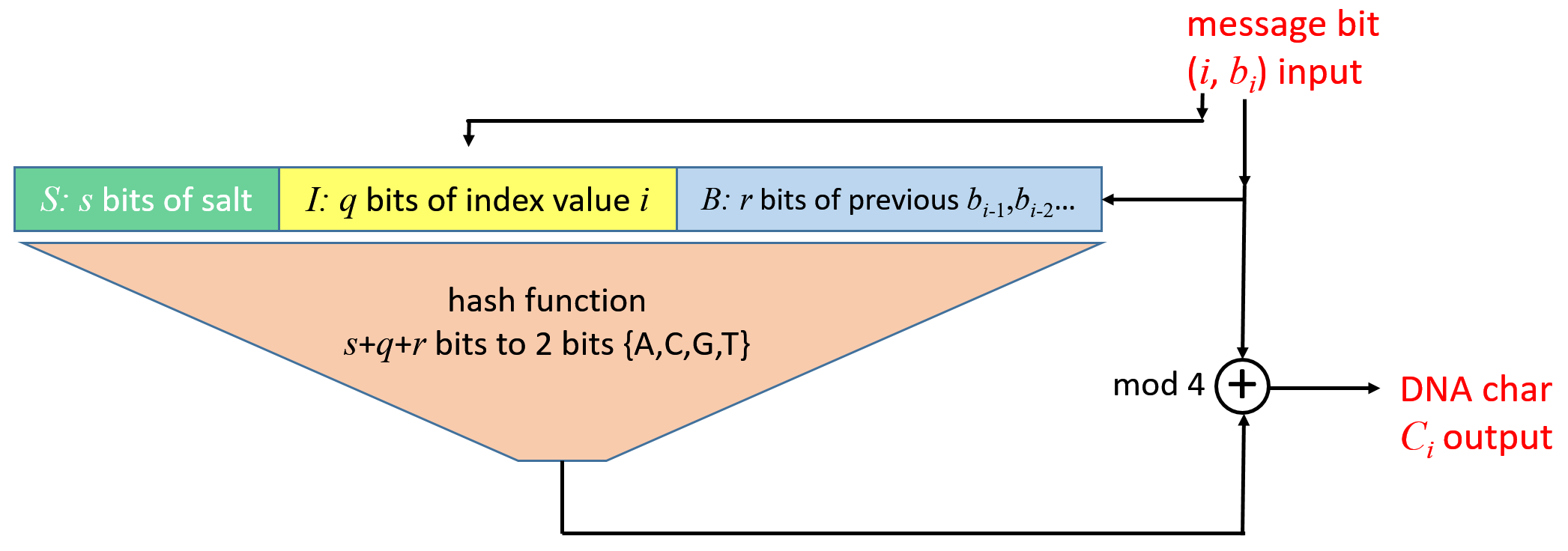
Finally, let be a deterministic hash function from bits to 2 bits
Then the formula for encoding is
| (2) |
Figure 2 shows the algorithm graphically.
Typical values that we use are , , , so that bits, a convenient value for input to the hash. For the hash function we use the low order 2 bits from the Numerical Recipes [18] function Ranhash.int64(), because it is very fast and will occur in the inner loop of the decode algorithm.
4.3 Decoding Algorithm
For simplicity, assume that error rates are “small”, so that “most” DNA bases are received as they were intended. (We will see in Section 5 that DNA character error rates up to %–% are tolerable.) Suppose we have correctly decoded and synchronized the message through bit and now want to know bit . Guessing the two possibilities, , we use equation (2) to predict two possibilities for the character . In the absence of an error, only one of these is guaranteed to agree with the observed character . We assign to a guess that generates disagreement with a penalty score equal (conceptually) to the negative log probability of observing a substitution error. In other words, a wrong guess might actually be right, but only if a substitution has occurred. If neither guess produces the correct , then both are assigned the substitution penalty.
We have not yet accounted for the possibility of insertions and deletions, however. In fact, there are more than the above two possible guesses. We must guess not just , but also a “skew” that tells us whether in comparing to we should skip characters () because of insertions, or posit missing characters () because of deletions (in which case there is no comparison to be done). As a practical simplification we consider only . (We comment on this simplification in Section 4.6.) Then there are six guesses for . Each can be scored by an appropriate log probability penalty for any implied substitution, insertion, or deletion.
Log probability penalties accumulate additively along any chain of guesses. In the causal case of a chain of all-correct guesses, we accumulate penalties only in the (relatively rare) case of actual errors. However, because of the way that the key (equation (2)) is constructed, single wrong guess for either , , or throws us into the acausal case where 3/4 of subsequent comparisons of computed (at some bit position index ) to observed (at some index ) will not agree—thus penalties will accumulate rapidly. The decoding problem, conceptually a maximum likelihood search, thus reduces to a shortest-path search in a tree with branching factor 6, but with the saving grace that the correct path will be much shorter than any deviation from it.

We can formalize the above discussion as follows. Let denote the joint hypothesis that the values are all correct and synchronize to the observed codestream character through equation (2). As a node in the search tree, the hypothesis spawns six child hypotheses, each of which can be scored with additional penalty (to be added to their common parent’s accumulated penalty) as follows:
| (3) |
Here can be thought of as respectively the log probability penalties for substitution, insertion, or deletion errors (but see Section 4.6). is the penalty or, if negative, reward, for an agreement between the computed and received codestream characters and . In the comparison notated above as , the index of is the first parameter in the hypothesis , while the index of is the last parameter in . Note that a child node’s is always computable from its parent’s and .
How can we practically search this huge tree? A conceptual starting point is the famous A* search algorithm [19], a best-first (that is, “greedy”) search utilizing a heap data structure. A* assigns a heuristic cost to every node that is the sum of its actual cost plus a quantity less than or equal to the smallest possible additional cost that it can incur in reaching the goal. (For a tree of constant depth, this is equivalent to adding a reward for every step taken closer to the leaf nodes, i.e., a negative constant above.) Figure 3 shows the logical flow of an A* search, and also the HEDGES decode algorithm. As already remarked, in coding theory, this kind of decoding strategy is called “sequential decoding”.
Provably, A* always finds the best path. For our application, unfortunately, it is exponentially slow, because actual errors along the true path cause too many spawned hypotheses to be revisited; and because its termination criterion is too restrictive, again leading to too many spawned hypotheses.
To ameliorate these problems we make two heuristic modifications of A*: First, we allow to be more negative than that sanctioned by A* and tune its value heuristically. While we thus lose the guarantee of finding exactly the shortest path, we heuristically encourage the search not to revisit earlier hypotheses after a sufficiently lengthy run of successes along one particular chain. Second, we adopt a “first past the post” termination criterion. That is, the first chain of hypotheses to decode the required bytes of message wins. It is not obvious (or, by us, provable) that these heuristics should result in a workable or efficient algorithm, but we will demonstrate by numerical experiment that it does.
4.4 Use of Salt to Protect Critical Message
Above, we noted the importance of protecting message bits that determine the ordering or “serial number” of strands for the outer, concatenated Reed-Solomon code. In equation (2) (and Figure 2) we allowed for some number of bits of known salt when message bit is encoded. Here is how this salt is enabling of extra protection: Suppose we want to protect an initial message bits. Then define recursively the salt by
| (4) |
Most errors in the first bits will be corrected as usual by the shortest-path heap search. But any residual error that gets through will “poison” the salt for the entire rest of the strand, rendering it undecodable. In effect we convert an error in the protected bits into an erasure of the whole strand. This may seem drastic, but it is just what we want: An strand with incorrect serial number (and hence incorrect ordering among other strands) would look like a strand of errors (with probablility 255/256 per byte) to the outer R-S; an erased strand is equivalent to only half as many errors.
4.5 Code Rates Other than One-Half
A simple modification of the encode and decode algorithms described in Sections 4.2 and 4.3 allows for code rates other than one-half. Take the input bitstream of expression (1) and partition it into a stream of values with variable numbers of bits in the range to , according to a repetitive pattern like the ones shown in Table 1.
| Code Rate | Pattern | (see text) |
|---|---|---|
| 0.750 | ||
| 0.600 | ||
| 0.500 | ||
| 0.333 | ||
| 0.250 | ||
| 0.166 |
Here are two examples showing how to interpret the entries in Table 1 (with adjacency denoting two-bit values in ):
Equation (2) for encoding now becomes
| (5) |
where is composed of concatenated previous variable bits. Pattern values of 0 provide one bit of additional redundancy check relative to the base case of code rate one-half, while pattern values of 2, encoding 2 bits per DNA character, provide one less bit. By construction the code rate is one-half the average of the integers in the pattern. The column in the table labeled will be explained in Section 4.6.
Decoding follows exactly the same pattern. Guessing a two-bit spawns 12 child hypotheses, while guessing a zero-bit spawns only 3.
4.6 Choice of, And Trade-Offs Among, Parameters
For encoding, the parameter choices are (i) the choice of code rate and variable bit pattern (as in Table 1), the default case being code rate ; (ii) the number of low-order bits of position index in the hash; (iii) the number of previous message bits in the hash; (iv) the number of salt bits; and (v) the number of initial message bits to be protected by salt.
It might at first seem that bigger is better for both and , but this is not the case. Restricting to a smaller value better allows the heap search to recover from previous errors, basically by finding an acasual (i.e., “wrong”) path that coincidentally puts it back on track. As for , restricting it to a smaller value could be useful in case one desires the capability of jumping into the middle of an undecoded message: The heap can then be initialized with all possible values of and (cf. Figure 2). For our system design, Section 3, this is not a necessary, or useful, capability, however. For the baseline validation experiments in Section 5, we take , , or .
For decoding, we need to know the encoding parameters, and must now also choose values for , and . While, conceptually, these are negative log probabilities of the occurrence of the different kinds of errors (which can be known only after the fact), we adopt a more empirical approach. First, we take to give the HEDGES decoding algorithm equal robustness against all three kinds of errors. Second, we note that the search for shortest path is invariant under applying the same linear (or affine) transformation to all four ’s. So, without loss of generality, we may take , leaving as the only free parameter. We determine optimal (or at least good) values for by numerical experiment. We find that the optimal depends only negligibly on the encoding parameters and , and only slightly on the length of the strand, but it does depend on the code rate. Good values for various code rates are given in the third column of Table 1.
Implicitly, the choice of reflects a tradeoff between computational workload and decode failure probability. that is too negative results in too greedy a search, which is fast but can get stuck in a blind alley that requires us to declare the rest of the strand as an erasure (hence its dependence on strand length). On the other hand, that is insufficiently negative results in a too large, potentially exponential, expansion of the size of the heap. Happily, there is an accessible range of workable values. Changes of % in matter little, and our values are implicitly tuned for best performance on strand lengths in the range to .
In Section 4.3 above we limited the guesses for to only so as to limit the expansion of the heap. This results in more than one consecutive insertion or deletion being improperly scored. For example, without the possibility of skew , the shortest available path through two deletions declares a spurious substitution . In practice, this makes little difference, because double deletions are significantly less common than single deletions, and because other, completely incorrect, paths score much worse.
It is an important point that choosing any set of decode parameters is not an irrevocable choice. Given a DNA message, one can make multiple tries, varying the decode parameters adaptively until acceptable performance is achieved. One can evaluate success by running time and by the count of errors needing correction by the outer R-S code. The parameter values that we suggest may be viewed as starting points.
5 Computer Validation Experiments
We have implemented HEDGES in C++ code, with also a Python interface for convenience. (We similarly implemented a compatible Python interface to the published “Schifra” implementation of Reed-Solomon.[20]) For tests on individual strands of length , we encode a random stream of message bits and degrade the resulting codestream by errors with a specified Poisson-random total rate, divided equally among the three error types, substitution, insertion, and deletion. Unless otherwise stated the HEDGES code rate is one-half.

We allow each decode a “hypothesis budget”, that is, a maximum size to which the heap is allowed to expand. If, along a strand, a decode exceeds its budget, we declare subsequent message bits in that strand to be erasures. Figure 4 shows examples of how decodes expend their budget along a long strand. There is a sharp bifurcation between decodable strands, which typically expend hypotheses per decoded bit, and undecodable strands, which go into blind alleys and readily expend hypotheses per decoded bit. The figure shows 10 selected examples of each type. In practice undecodable strands are much rarer than decodable ones.


Figure 5 shows decode failure rates actually achieved by a half-rate code, as a function of length of strand, input total error rate, and hypothesis budget. One sees that, for strand lengths in the useful range 100–1000, failure rates are readily achievable for total input error rates up to %. For an input error rate of 3%, strand lengths up to are feasible. Failure rates are easily absorbed as erasures in the error budget of an outer, interleaved Reed-Solomon code (see below, this section).
In the case of a successful decode, there may remain uncorrected substitution errors. Figure 6 shows the uncorrected (output) bit, and byte, error rates along strands of length 240 for the three input codestream character error rates 3%, 5%, and 10%. The uncorrected error rates vary along the strand for two reasons: First, for this experiment, we applied salt protection to the first 24 message bits (that is, 24 characters for the half-rate code). One sees that this worked as advertised: There were no uncorrected errors in the first 24 bits. Second, uncorrected error rates are seen to rise as the length of the strand is approached. Although undesirable, this is an inevitable feature of HEDGES. As the strand end is approached, there are fewer redundancy checks available downstream, making the greedy search algorithm less selective. Our system design (Section 3) allows for specifying some number of “runout” bits at the ends of the strands, encoding zeros and not part of the message packet. How much runout to allow depends on how much one wants to burden the R-S error budget. For this numerical experiment, we assumed 24 runout bits.
It is notable that the byte error rates in Figure 6 are only times the bit error rates, rather than times (depending on the bit error rate) if the errors were randomly distributed. This shows that HEDGES’s uncorrected errors are bursty, which is good for input to R-S and gains some overall efficiency.
Exclusive of the salt-protected and runout regions, the uncorrected bit error rates for this experiment are about , , for input error rates 3%, 5%, and 10%, respectively. The corresponding byte error rates are , , and .
What level of uncorrected errors may we allow to get through to the R-S outer code, with a high probability that they will there be corrected? is able to correct 16 byte-errors, or any combination of byte errors and erasures whose equivalent number is
The probability of failure to completely correct 255 bytes, for Poisson random byte errors/erasures is thus the cumulative probability
| (6) |
where is the byte error rate (B.e.r.) plus half the erasure rate. As mentioned above, we interleave and apply the R-S code diagonally (see Figure 1) because (i) strands may be missing, (ii) byte errors along a single strand may be bursty, and (iii) it is found experimentally that sequencing and synthesis error rates can be different (often larger) near to the end of strands. The interleaved diagonal pattern ensures that no single length R-S packet gets handicapped by an error rate much different than the average across the whole strand, and that its number of errors will be distributed with (close to) Poisson statistics. Table 2 evaluates equation (6) for relevant values of . One sees that a value are adequate to guarantee error-free decoding of messages of gigabyte length or longer.

| 0.005 | |
|---|---|
| 0.010 | |
| 0.020 | |
| 0.030 | |
| 0.040 |
Figure 7 now shows the results of a numerical experiment evaluating as a function of input DNA error rates for six different code rates. The evaluation was done with strand length (as a variant of the value in Figure 6), no salt protection, and 2 bytes of runout on each strand (errors in which are not counted). Using Table 2, one sees that a DNA error rate of about 1% is correctable at code rate 3/4 with probability effectively 1, increasing to a correctable error rate of about 15% at code rate 1/6.
6 Channel Capacity re Shannon Limit
We might wonder how close the results of Figure 7 come to the absolute bound of the Shannon limiting channel capacity [1]. Unfortunately, computing the Shannon limit for even the simplest case of a binary deletion channel, let alone channels with also insertions and substitutions, remains a difficult unsolved problem [6, 22]. Still, it is possible to get some idea by making an informed estimate as follows.

A remarkable theorem of Shannon [21] proves that the channel capacity of a forward error-corrected channel is identical to that of a “feedback channel,” where the sender gets to see (error-free) what was actually received, and then send correcting information post hoc. We can thus estimate channel capacity by reducing the maximum capacity (for DNA, 2 bits per character) by the entropy of the necessary correction messages. The reason that this is an estimate only (strictly, a lower bound), is that we may not be sending the optimally short correction messages, especially as the error rate becomes large.
In our case, suppose is the character error rate. As before, assume equal probabilities for the three kinds of errors. Then we can estimate the Shannon limit of the channel as
| (7) |
where is the entropy of a binary choice,
| (8) |
In equation (7), the first term in brackets is the cost of communicating whether a particular code character marks the position of an error. The second term is the cost of telling which kind of error (substitution, deletion, insertion). The third term is the cost of communicating the missing character in a deletion. The fourth is the similar cost for a substitution. While strictly only a lower bound, analogous results for binary deletion channels [22] suggest that equation (7) is actually a good approximation for small values of .
We now calculate the channel capacity actually achievable with HEDGES by the relation
| (9) |
Here the factor 2 is the number of bits per DNA character, while the factor in square brackets reflects the loss of channel capacity to an (assumed perfect) concatenated outer code that corrects all of HEDGES’ uncorrected bit errors.
Figure 8 shows the results of the comparison. One sees that HEDGES achieves a respectable fraction, , of the estimated Shannon limit for DNA character error rates up to 20%.
7 Discussion
Previous work on DNA information storage, despite the increasing sophistication of methods, has largely ignored the possibility of directly correcting insertion and deletion errors by an appropriate error-correcting code. Instead, most previous work has relied on multiple sequence alignment after sequencing DNA messages to significant depths. In effect, though not always acknowledged, this method is an inefficient multiple-repetition code.
This paper developed a coding technique, termed HEDGES, for the direct correction of insertions and deletions, along with substitutions, workable with (combined) DNA character error rates up to 20%, and at a respectable fraction of the Shannon information limit. The code, HEDGES, was optimized for use as the inner code in an overall design with an outer concatenated code that will generally be interleaved across DNA strands. Used with HEDGES, the outer code need not be indel-aware and can be a conventional ECC like Reed-Solomon.
Acknowledgments
We have benefitted from communication with Dave Forney, Dan Costello, and Vince Poor, and from our continuing collaboration in related matters with Ilya Finkelstein and Stephen Jones.
References
- [1] Shannon CE, Weaver W, The Mathematical Theory of Communication (University of Illinois Press, 1949)
- [2] MacWilliams FJ, Sloane NJA, The Theory of Error-Correcting Codes (North Holland, 1983)
- [3] Roth RM, Introduction to Coding Theory (Cambridge University Press, 2006)
- [4] Moon TK, Error Correction Coding: Mathematical Methods and Algorithms (Wiley, 2005)
- [5] Lin S, Costello DJ Error Control Coding, Second Edition (Pearson, 2004)
- [6] Mitzenmacher, M, “A survey of results for deletion channels and related synchronization channels”, Probability Surveys, vol. 6, pp. 1-33 (2009)
- [7] Li R, New developments in coding against insertions and deletions, Honors Thesis, Carnegie Mellon University, at https://www-cs.stanford.edu/ rayyli/static/paper/RayLi_HonorsThesis_20170828.pdf
- [8] Hawkins JA, Jones SK, Finkelstein IJ, Press WH, “Indel-correcting DNA barcodes for high-throughput sequencing”, PNAS, 115 (27), pp. E6217-E6226 (2018)
- [9] Wicker SB, Bhargava VK, An Introduction to Reed-Solomon Codes (Wiley-IEEE, 1994)
- [10] Church GM, Gao Y, Kosuri S, “Next-Generation Digital Information Storage in DNA”, Science, vol. 337, pp. 1628 (2012)
- [11] Goldman N, Bertone P, Chen S, Dessimoz C, LeProust EM, Sipos B, Birney E, “Towards Practical, High-Capacity, Low-Maintenance Information Storage in Synthesized DNA”, Nature, vol. 494, pp. 77–80 (2013)
- [12] Grass RN, Heckel R, Pudda M, Paunescu D, Stark WJ, “Robust Chemical Preservation of Digital Information on DNA in Silica with Error-Correcting Codes”, Angew. Chem. Int. Ed., vol. 54, pp. 2552–2555 (2015)
- [13] Bornholt J, Lopez R, Carmean DM, Ceze L, Seelig G, Strauss K, “A DNA-Based Archival Storage System”, ACM SIGARCH Computer Architecture News, vol. 44, pp. 637-649 (2016).
- [14] Erlich Y, Zielinski D, “DNA Fountain enables a robust and efficient storage architecture”, Science, vol. 255, pp. 950–954 (2017)
- [15] Yazdi SMHT, Gabrys R, Milenkovic O, “Portable and Error-Free DNA-Based Data Storage”, Nature Scientific Reports, 7:5011 (2017)
- [16] Organick L, Ang SD, Chen Y-J, et al., “Random access in large-scale DNA data storage”, Nature Biotechnology, vol. 36, no. 3, pp. 242–248 (2018)
- [17] Vigenère, Blaise de, Traicté des chiffres ou secrètes manières d’escrire, Abel l’Angelier, Paris 1586. ff. 46r-49v. See also Wikipedia, “Autokey cipher”.
- [18] Press WH, Teukolsky SA, Vetterling WT, Flannery BP, Numerical Recipes: The Art of Scientific Computing, Third Edition (Cambridge University Press, 2007), p. 352.
- [19] Hart PE, Nilsson NJ, Raphael B, ”A Formal Basis for the Heuristic Determination of Minimum Cost Paths”, IEEE Transactions on Systems Science and Cybernetics, SSC4, vol. 4 no. 2, pp. 100-107 (1968)
- [20] Partow A, Schifra Reed-Solomon Code Library, at http://www.schifra.com.
- [21] Shannon CE, “The Zero Error Capacity of a Noisy Channel”, IRE Transactions on Information Theory vol. 2, no. 3, pp. 8–19 (1956).
- [22] Rahmati M, Duman TM, “Upper Bounds on the Capacity of Deletion Channels Using Channel Fragmentation”, IEEE Transactions on Information Theory, vol. 61, no. 1 (2015)