Local Obfuscation Mechanisms for Hiding Probability Distributions Thanks: This work was partially supported by JSPS KAKENHI Grant JP17K12667, JP19H04113, and Inria LOGIS project.

We denote by $\mathbb{D}\mathcal{X}$ the set of all probability distributions over a set $\mathcal{X}$, and by $|\mathcal{X}|$ the number of elements in a finite set $\mathcal{X}$.

Given a finite set $\mathcal{X}$ and a distribution $\lambda\in\mathbb{D}\mathcal{X}$, the probability of drawing a value $x$ from $\lambda$ is denoted by $\lambda[x]$. For a finite subset $\mathcal{X}^{\prime}\subseteq\mathcal{X}$ we define $\lambda[\mathcal{X}^{\prime}]$ by: $\lambda[\mathcal{X}^{\prime}]=\sum_{x^{\prime}\in\mathcal{X}^{\prime}}\lambda[x^{\prime}]$. For a distribution $\lambda$ over a finite set $\mathcal{X}$, its support $\mathsf{supp}(\lambda)$ is defined by $\mathsf{supp}(\lambda)=\{x\in\mathcal{X}\colon\lambda[x]>0\}$. Given a $\lambda\in\mathbb{D}\mathcal{X}$ and a $f:\mathcal{X}\rightarrow\mathbb{R}$, the expected value of $f$ over $\lambda$ is: $\operatornamewithlimits{\mathbb{E}}_{x\sim\lambda}[f(x)]\stackrel{{\scriptstyle\mathrm{def}}}{{=}}\sum_{x\in\mathcal{X}}\lambda[x]f(x)$.

For a randomized algorithm $\mathit{A}:\mathcal{X}\rightarrow\mathbb{D}\mathcal{Y}$ and a set $R\subseteq\mathcal{Y}$ we denote by $\mathit{A}(x)[R]$ the probability that given input $x$, $\mathit{A}$ outputs one of the elements of $R$. Given a randomized algorithm $\mathit{A}:\mathcal{X}\rightarrow\mathbb{D}\mathcal{Y}$ and a distribution $\lambda$ over $\mathcal{X}$, we define ${\mathit{A}}^{\#}(\lambda)$ as the distribution of the output of $\mathit{A}$. Formally, for a finite set $\mathcal{X}$, the lifting of $\mathit{A}$ w.r.t. $\mathcal{X}$ is the function ${\mathit{A}}^{\#}:\mathbb{D}\mathcal{X}\rightarrow\mathbb{D}\mathcal{Y}$ such that ${\mathit{A}}^{\#}(\lambda)[R]\stackrel{{\scriptstyle\mathrm{def}}}{{=}}\sum_{x\in\mathcal{X}}\lambda[x]\mathit{A}(x)[R]$.

Differential privacy [1] captures the idea that given two “adjacent” inputs $x$ and $x^{\prime}$ (from a set $\mathcal{X}$ of data with an adjacency relation $\varPhi$), a randomized algorithm $\mathit{A}$ cannot distinguish $x$ from $x^{\prime}$ (with degree of $\varepsilon$ and up to exceptions $\delta$).

Differential privacy can be achieved by a privacy mechanism, namely a randomized algorithm that adds probabilistic noise to a given input that we want to protect. The amount of noise added by some popular mechanisms (e.g., the exponential mechanism) depends on a utility function $\mathit{u}:\mathcal{X}\times\mathcal{Y}\rightarrow\mathbb{R}$ that maps a pair of input and output to a utility score. More precisely, the noise is added according to the “sensitivity” of $\mathit{u}$, which we define as follows.

Note that $\mathit{d}$ is a pseudometric. Hereafter we assume that for all $x,y$, $\mathit{u}(x,y)=0$ is logically equivalent to $x=y$. Then the utility distance $\mathit{d}$ is a metric.

We review the notion of extended differential privacy [15], which relaxes DP by incorporating a metric $d$. Intuitively, this notion guarantees that when two inputs $x$ and $x^{\prime}$ are closer in terms of $d$, the output distributions are less distinguishable.

We recall the notion of probability coupling as follows.

We then recall the $\infty$-Wasserstein metric [16] between two distributions.

The $\infty$-Wasserstein metric $\mathit{W}_{\infty,\mathit{d}}(\lambda_{0},\lambda_{1})$ represents the minimum largest move between points in a transportation from $\lambda_{0}$ to $\lambda_{1}$. Specifically, in a transportation $\gamma$,  $\max_{(x_{0},x_{1})\in\mathsf{supp}(\gamma)}\allowbreak\mathit{d}(x_{0},x_{1})$ represents the largest move from a point in $\lambda_{0}$ to another in $\lambda_{1}$. For instance, in the coupling $\gamma$ in Example 1, the largest move is $1$ (from $\lambda_{0}[2]$ to $\lambda_{1}[1]$, and from $\lambda_{0}[2]$ to $\lambda_{1}[3]$). Such a largest move is minimized by a coupling that achieves the $\infty$-Wasserstein metric. We denote by $\mathit{\Gamma_{\!{\rm\infty,\mathit{d}}}}$ the set of all couplings that achieve the $\infty$-Wasserstein metric.

Finally, we recall the notion of the lifting of relations.

Note that by Definition 5, the coupling $\gamma$ is a probability distribution over $\varPhi$ whose marginal distributions are $\lambda_{0}$ and $\lambda_{1}$. If $\varPhi=\mathcal{X}\times\mathcal{X}$, then ${\varPhi}^{\#}=\mathbb{D}\mathcal{X}\times\mathbb{D}\mathcal{X}$.

As a running example, we consider an LBS (location based service) in which each user queries an LBS provider for a list of shops nearby. To hide a user’s exact location $x$ from the provider, the user applies a randomized algorithm $\mathit{A}:\mathcal{X}\rightarrow\mathbb{D}\mathcal{Y}$, called a local obfuscation mechanism, to her location $x$, and obtains an approximate information $y$ with the probability $\mathit{A}(x)[y]$.

To illustrate the privacy of attributes, let us consider an example in which users try to prevent an attacker from inferring whether they are ${\it male}$ or ${\it female}$ by obfuscating their own exact locations using a mechanism $\mathit{A}$. For each $t\in\{{\it male},{\it female}\}$, let $\lambda_{t}\in\mathbb{D}\mathcal{X}$ be the prior distribution of the location of the users who have the attribute $t$. Intuitively, $\lambda_{{\it male}}$ (resp. $\lambda_{{\it female}}$) represents an attacker’s belief on the location of the male (resp. female) users before the attacker observes an output of the mechanism $\mathit{A}$. Then the privacy of $t$ can be modeled as a property that the attacker has no idea on whether the actual location $x$ follows the distribution $\lambda_{{\it male}}$ or $\lambda_{{\it female}}$ after observing an output $y$ of $\mathit{A}$.

This can be formalized in terms of $\varepsilon$-local DP. For each $t\in\{{\it male},\allowbreak{\it female}\}$,  we denote by $p(y\,|\,\lambda_{t})$ the probability of observing an obfuscated location $y$ when an actual location $x$ is distributed over $\lambda_{t}$, i.e., $p(y\,|\,\lambda_{t})=\sum_{x\in\mathcal{X}}\lambda_{t}[x]\mathit{A}(x)[y]$. Then we can define the privacy of $t$ by:

We generalize the privacy of attributes (in Section 3.1) and define the notion of distribution privacy (DistP) as the differential privacy where the input is a probability distribution of data rather than a value of data. This notion models a level of obfuscation that hides which distribution a data value is drawn from. Intuitively, we say a randomized algorithm $\mathit{A}$ provides DistP if, by observing an output of $\mathit{A}$, we cannot detect from which distribution an input to $\mathit{A}$ is generated.

For example, the privacy of a user attribute $t\in\{{\it male}{},\allowbreak{\it female}{}\}$ described in Section 3.1 can be formalized as $(\varepsilon,0)$-DistP w.r.t. $\{\lambda_{{\it male}},\lambda_{{\it female}}\}$.

Mathematically, DistP is not a new notion but the DP for distributions. To contrast with DistP, we refer to the DP for data values as point privacy.

Next we introduce an extended form of distribution privacy to a metric. Intuitively, extended distribution privacy guarantees that when two input distributions are closer, then the output distributions must be less distinguishable.

The interpretation of DP has been explored in previous work [17, 15] using the notion of Bayes factor. Similarly, the meaning of DistP can also be explained in terms of Bayes factor, which compares the attacker’s prior and posterior beliefs.

Assume that an attacker has some belief on the input distribution before observing the output values of an obfuscater $\mathit{A}$. We denote by $p(\lambda)$ the prior probability that a distribution $\lambda$ is chosen as the input distribution. By observing an output $y$ of $\mathit{A}$, the attacker updates his belief on the input distribution. We denote by $p(\lambda|y)$ the posterior probability of $\lambda$ being chosen, given an output $y$.

For two distributions $\lambda_{0},\lambda_{1}$, the Bayes factor $K(\lambda_{0},\allowbreak\lambda_{1},y)$ is defined as the ratio of the two posteriors divided by that of the two priors: $K(\lambda_{0},\lambda_{1},y)=\frac{p(\lambda_{0}|y)}{p(\lambda_{1}|y)}\big/\frac{p(\lambda_{0})}{p(\lambda_{1})}$. If the Bayes factor is far from $1$ the attacker significantly updates his belief on the distribution by observing a perturbed output $y$ of $\mathit{A}$.

Assume that $\mathit{A}$ provides $(\varepsilon,0)$-DistP. By Bayes’ theorem, we obtain:

Intuitively, if the attacker believes that $\lambda_{0}$ is $k$ times more likely than $\lambda_{1}$ before the observation, then he believes that $\lambda_{0}$ is $k\cdot e^{\varepsilon}$ times more likely than $\lambda_{1}$ after the observation. This means that for a small value of $\varepsilon$, DistP guarantees that the attacker does not gain information on the distribution by observing $y$.

In the case of XDistP, the Bayes factor $K(\lambda_{0},\lambda_{1},y)$ is bounded above by $e^{\varepsilon d(\lambda_{0},\lambda_{1})}$. Hence the attacker gains more information for a larger distance $d(\lambda_{0},\lambda_{1})$.

In the previous sections, we assume that we know the distance between two actual input distributions, and can determine the amount of noise required for distribution obfuscation. However, an attacker may have different beliefs on the distributions that are closer to the actual ones, e.g., more accurate distributions obtained by more observations and specific situations (e.g., daytime/nighttime).

To see this, for each $\lambda\in\mathbb{D}\mathcal{X}$, let $\tilde{\lambda}$ be an attacker’s belief on $\lambda$. We say that an attacker has $(c,\mathit{d})$-close beliefs if each distribution $\lambda$ satisfies $\mathit{d}(\lambda,\tilde{\lambda})\leq c$. Then extended distribution privacy in the presence of an attacker is given by:

When the attacker’s beliefs are closer to ours, then $c$ is smaller, hence a stronger distribution privacy is guaranteed. See Appendix 0.B.2 for DistP. Note that assuming some attacker’s beliefs are inevitable also in many previous studies, e.g., when we want to protect the privacy of correlated data [18, 19, 20].

Finally, we present a brief remark on the difference between DistP and the differential privacy of histogram publication (e.g., [21]). Roughly, a histogram publication mechanism is a central mechanism that aims at hiding a single record $x\in\mathcal{X}$ and outputs an obfuscated histogram, e.g., a distribution $\mu\in\mathbb{D}\mathcal{Y}$, whereas a DistP mechanism is a local mechanism that aims at hiding an input distribution $\lambda\in\mathbb{D}\mathcal{X}$ and outputs a single perturbed value $y\in\mathcal{Y}$.

Note that neither of these implies the other. The $\varepsilon$-DP of a histogram publication mechanism means that for any two adjacent inputs $x,x^{\prime}\in\mathcal{X}$ and any histogram $\mu\in\mathbb{D}\mathcal{Y}$, $\frac{p(\mu|x)}{p(\mu|x^{\prime})}\leq e^{\varepsilon}.$ However, this does not derive $\varepsilon$-DistP, i.e., for any adjacent input distributions $\lambda,\lambda^{\prime}\in\mathbb{D}\mathcal{X}$ and any output $y\in\mathcal{Y}$, $\frac{p(y|\lambda)}{p(y|\lambda^{\prime})}\leq e^{\varepsilon}$.

We first show every DP mechanism provides DistP. (See Definition 7 for ${\varPhi}^{\#}$.)

This means that the mechanism $\mathit{A}$ makes any pair $(\lambda_{0},\lambda_{1})\in{\varPhi}^{\#}$ indistinguishable up to the threshold $\varepsilon$ and with exceptions $\delta\cdot|\varPhi|$. Intuitively, when $\lambda_{0}$ and $\lambda_{1}$ are adjacent w.r.t. the relation ${\varPhi}^{\#}$, we can construct $\lambda_{1}$ from $\lambda_{0}$ only by moving mass from $\lambda_{0}[x_{0}]$ to $\lambda_{1}[x_{1}]$ where $(x_{0},x_{1})\in\varPhi$ (i.e., $x_{0}$ is adjacent to $x_{1}$).

Compared to DP mechanisms, XDP mechanisms are known to provide better utility. Alvim et al. [23] show the planar Laplace mechanism [3] adds less noise than the randomized response, since XDP hides only closer locations. However, we show XDP mechanisms still need to add much noise proportionally to the $\infty$-Wasserstein distance between the distributions we want make indistinguishable.

We first define the tupling mechanism as a local mechanism that obfuscates a given input $x$ by using a point perturbation mechanism $\mathit{A}$ (not necessarily in terms of DP or XDP), and that also adds $k$ random dummies $r_{1},r_{2},\ldots,r_{k}$ to the output to obfuscate the input distribution (Algorithm 1).

The probability that given an input $x$, the mechanism $\mathit{Q}^{\sf tp}_{k,\nu,\mathit{A}}$ outputs $\bar{y}$ is given by $\mathit{Q}^{\sf tp}_{k,\nu,\mathit{A}}(x)[\bar{y}]$.

Next we show that the tupling mechanism provides DistP w.r.t. the following class of distributions. Given $\beta,\eta\in[0,1]$ and $\mathit{A}:\mathcal{X}\rightarrow\mathbb{D}\mathcal{Y}$, we define $\Lambda_{\beta,\eta,\mathit{A}}$ by:

For instance, a distribution $\lambda$ satisfying $\max_{x}\lambda[x]\leq\beta$ belongs to $\Lambda_{\beta,0,\mathit{A}}$. (See Proposition 12 in Appendix 0.B.8.)

This claim states that just adding random dummies achieves DistP without any assumption on $\mathit{A}$ (e.g., $\mathit{A}$ does not have to provide DP). For a smaller range size $|\mathcal{Y}|$ and a larger number $k$ of dummies, we obtain a stronger DistP.

Note that the distributions protected by $\mathit{Q}^{\sf tp}_{k,\nu,\mathit{A}}$ belong to the set $\Lambda_{\beta,\eta,\mathit{A}}$.

• •

  When $\beta=1$, $\Lambda_{\beta,\eta,\mathit{A}}$ is the set of all distributions (i.e., $\Lambda_{1,\eta,\mathit{A}}=\mathbb{D}\mathcal{X}$) while $\varepsilon_{\alpha}$ and $\delta_{\alpha}$ tend to be large.

• •

  For a smaller $\beta$, the set $\Lambda_{\beta,\eta,\mathit{A}}$ is smaller while $\varepsilon_{\alpha}$ and $\delta_{\alpha}$ are smaller; that is, the mechanism provides a stronger DistP for a smaller set of distributions.

• •

  If $\mathit{A}$ provides $\varepsilon_{\mathit{A}}$-DP,  $\Lambda_{\beta,\eta,\mathit{A}}$ goes to $\mathbb{D}\mathcal{X}$ for $\varepsilon_{\mathit{A}}\rightarrow 0$. More generally, $\Lambda_{\beta,\eta,\mathit{A}}$ is larger when the maximum output probability $\max_{y}{\mathit{A}}^{\#}(\lambda)[y]$ is smaller.

In practice, even when $\varepsilon_{\mathit{A}}$ is relatively large, a small number of dummies enables us to provide a strong DistP, as shown by experiments in Section 7.

We note that Theorem 3 may not imply DP of the tupling mechanism, depending on $\mathit{A}$. For example, suppose that $\mathit{A}$ is the identity function. For small $\varepsilon_{\alpha}$ and $\delta_{\alpha}$, we have $\beta\ll 1$, hence no point distribution $\lambda$ (where $\lambda[x]=1$ for some $x$) belongs to $\Lambda_{\beta,\eta,\mathit{A}}$, namely, the tupling mechanism does not provide $(\varepsilon_{\alpha},\delta_{\alpha})$-DP.

When a mechanism outputs a value $y$ closer to the original input $x$, she obtains a larger utility, or equivalently, a smaller service quality loss $\mathit{d}(x,y)$. For example, in an LBS (location based service), if a user located at $x$ submits an obfuscated location $y$, the LBS provider returns the shops near $y$, hence the service quality loss can be expressed as the Euclidean distance $\mathit{d}(x,y)\stackrel{{\scriptstyle\mathrm{def}}}{{=}}\|x-y\|$.

Since each output of the tupling mechanism consists of $k+1$ elements, the quality loss of submitting a tuple $\bar{y}=(y_{1},y_{2},\ldots,y_{k+1})$ amounts to $\mathit{d}(x,\bar{y})\mathbin{:=}\min_{i}\allowbreak\mathit{d}(x,y_{i})$. Then the expected quality loss of the mechanism is defined as follows.

For a larger number $k$ of random dummies, $\min_{i}\allowbreak\mathit{d}(x,y_{i})$ is smaller on average, hence $L\bigl(\mathit{Q}^{\sf tp}_{k,\nu,\mathit{A}}\bigr)$ is also smaller. Furthermore, thanks to the distribution obfuscation by random dummies, we can instead reduce the perturbation noise added to the actual input $x$ to obtain the same level of DistP. Therefore, the service quality is much higher than existing mechanisms, as shown in Section 7.

As a point obfuscation mechanism $\mathit{A}$ used in the tupling mechanism $\mathit{Q}^{\sf tp}_{k,\nu,\mathit{A}}{}$, we define the restricted Laplace (RL) mechanism below. Intuitively, $(\varepsilon_{\!\mathit{A}},r)$-RL mechanism adds $\varepsilon_{\!\mathit{A}}$-XDP Laplace noise only within a radius $r$ of the original location $x$. This ensures that the worst-case quality loss of the tupling mechanisms is bounded above by the radius $r$, whereas the standard Laplace mechanism reports a location $y$ that is arbitrarily distant from $x$ with a small probability.

Since the support of $\mathit{A}$ is limited to $\mathcal{Y}_{x,r}$, $\mathit{A}$ provides better service quality but does not provide DP. Nevertheless, as shown in Theorem 3,  $\mathit{Q}^{\sf tp}_{k,\nu,\mathit{A}}{}$ provides DistP, due to dummies in $\mathcal{Y}\setminus\mathcal{Y}_{x,r}$. This implies that DistP is a relaxation of DP that guarantees the privacy of attributes while achieving higher utility by weakening the DP protection of point data. In other words, DistP mechanisms are useful when users want both to keep high utility and to protect the attribute privacy more strongly than what a DP mechanism can guarantee (e.g., when users do not mind revealing their actual locations outside home, but want to hide from robbers the fact that they are outside home, as motivated in Section 1).

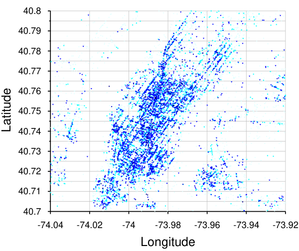
We perform experiments on location privacy in Manhattan by using the Foursquare dataset (Global-scale Check-in Dataset) [24]. We first divide Manhattan into $11\times 10$ regions with $1.0\mathrm{km}$ intervals. To provide more useful information to users in crowded regions, we further re-divide these regions to $276$ regions by recursively partitioning each crowded region into four until each resulting region has roughly similar population density.²² 2 This partition may be useful to achieve smaller values $(\varepsilon,\delta)$ of DistP, because $\beta$ tends to be smaller when the population density is closer to the uniform distribution. Let $\mathcal{Y}$ be the set of those $276$ regions, and $\mathcal{X}$ be the set of the $228$ regions inside the central $10\mathrm{km}\times 9\mathrm{km}$ area in $\mathcal{Y}$.

As an obfuscation mechanism $Q$, we use the tupling mechanism $\mathit{Q}^{\sf tp}_{k,\nu,\mathit{A}}{}$ that uses an $(\varepsilon_{\!\mathit{A}},r)$-RL mechanism $\mathit{A}$ and the uniform distribution $\nu$ over $\mathcal{Y}$ to generate dummy locations. Note that $\nu$ is close to the population density distribution over $\mathcal{Y}$, because each region in $\mathcal{Y}$ is constructed to have roughly similar population density. In the definitions of the RL mechanism and the quality loss, we use the Euclidean distance $\|\cdot\|$ between the central points of the regions.

In the experiments, we measure the privacy of user attributes, formalized as DistP. For example, let us consider the attribute ${\it male}/{\it female}$. For each $t\in\{{\it male},{\it female}\}$, let $\lambda_{t}\in\mathbb{D}\mathcal{X}$ be the prior distribution of the location of the users having the attribute $t$. Then, $\lambda_{{\it male}}$ (resp. $\lambda_{{\it female}}$) represents an attacker’s belief on the location of the male (resp. female) users. We define these as the empirical distributions that the attacker can calculate from the above Foursquare dataset.

We define the attack success rate (ASR) as the ratio that the attacker succeeds to infer a user has an attribute when she does actually. We use an inference algorithm based on the Bayes decision rule [25] to minimize the identification error probability when the estimated posterior probability is accurate [25].

In Fig. 5, we show the relationships between DistP and ASR in Manhattan for the attribute home, meaning the users located at their home. In theory, $\rm{ASR}=0.5$ represents the attacker learns nothing about the attribute, whereas the empirical ASR in our experiments fluctuates around $0.5$. This seems to be caused by the fact that the dataset and the number of locations are finite. From Fig. 5, we conclude that $\varepsilon=1$ is an appropriate parameter for $(\varepsilon,0.001)$-DistP to achieve $\rm{ASR}=0.5$ in our setting, and we confirm this for other attributes. However, we note that this is an empirical criterion possibly depending on our setting, and the choice of $\varepsilon$ for DistP can be as controversial as that for DP and should also be investigated using approaches for DP (e.g., [26]) in future work.

In Appendices 0.A.1, 0.A.2, and 0.A.3, we show that different levels of DistP are achieved for different attributes in different cities. In particular, we present appropriate parameters for the tupling mechanism for various attributes in a couple of cities.

We demonstrate that the tupling mechanism (TM) outperforms the popular mechanisms: the randomized response (RR), the planar Laplace (PL), and the planar Gaussian (PG). In Fig. 5 we compare these concerning the relationship between $\varepsilon$-DistP and expected quality loss. Since PG always has some $\delta$, it provides a weaker DistP than PL for the same quality loss. We also confirm that PL has smaller loss than RR, since it adds noise proportionally to the distance. Comparison using other attributes can be found in Appendix 0.A.1.

Finally, we briefly discuss the computational cost of the tupling mechanism $\mathit{Q}^{\sf tp}_{k,\nu,\mathit{A}}{}$, compared to $\rm{PL}{}$. In the implementation, for a larger domain $\mathcal{X}$,  $\rm{PL}{}$ deals with a larger size $|\mathcal{X}|\times|\mathcal{Y}|$ of the mechanism’s matrix, since it outputs each region with a non-zero probability. In contrast, since the RL mechanism $\mathit{A}$ used in $\mathit{Q}^{\sf tp}_{k,\nu,\mathit{A}}{}$ maps each location $x$ to a region within a radius $r$ of $x$, the size of $\mathit{A}$’s matrix is $|\mathcal{X}|\times|\mathcal{Y}_{x,r}|$, requiring much smaller memory space than $\rm{PL}{}$.

Furthermore, the users of $\rm{TM}{}$ can simply ignore the responses to dummy queries, whereas the users of $\rm{PL}{}$ need to select relevant POIs (point of interests) from a large radius of $x$, which could cost computationally for many POIs. Therefore, $\rm{TM}{}$ is more suited to be used in mobile environments than $\rm{PL}{}$.

References

• [1] C. Dwork, “Differential privacy,” in Proc. ICALP, 2006, pp. 1–12.
• [2] J. C. Duchi, M. I. Jordan, and M. J. Wainwright, “Local privacy and statistical minimax rates,” in Proc. FOCS, 2013, pp. 429–438.
• [3] M. E. Andrés, N. E. Bordenabe, K. Chatzikokolakis, and C. Palamidessi, “Geo-indistinguishability: differential privacy for location-based systems,” in Proc. CCS. ACM, 2013, pp. 901–914.
• [4] Úlfar Erlingsson, V. Pihur, and A. Korolova, “RAPPOR: Randomized aggregatable privacy-preserving ordinal response,” in Proc. CCS, 2014, pp. 1054–1067.
• [5] N. E. Bordenabe, K. Chatzikokolakis, and C. Palamidessi, “Optimal geo-indistinguishable mechanisms for location privacy,” in Proc. CCS, 2014, pp. 251–262.
• [6] L. Liao, D. Fox, and henry Kautz, “Extracting places and activities from GPS traces using hierarchical conditional random fields,” Int. J. Robotics Res., vol. 1, no. 26, pp. 119–134, 2007.
• [7] V. W. Zheng, Y. Zheng, and Q. Yang, “Joint learning user’s activities and profiles from GPS data,” in Proc. LBSN, 2009, pp. 17–20.
• [8] Y. Matsuo, N. Okazaki, K. Izumi, Y. Nakamura, T. Nishimura, and K. Hasida, “Inferring long-term user properties based on users’ location history,” in Proc. IJCAI, 2007, pp. 2159–2165.
• [9] D. Yang, B. Qu, and P. Cudré-Mauroux, “Privacy-preserving social media data publishing for personalized ranking-based recommendation,” IEEE Trans. Knowl. Data Eng., vol. 31, no. 3, pp. 507–520, 2019.
• [10] J. Otterbacher, “Inferring gender of movie reviewers: Exploiting writing style, content and metadata,” in Proc. CIKM, 2010, pp. 369–378.
• [11] U. Weinsberg, S. Bhagat, S. Ioannidis, and N. Taft, “BlurMe: Inferring and obfuscating user gender based on ratings,” in Proc. RecSys, 2012, pp. 195–202.
• [12] N. Z. Gong and B. Liu, “Attribute inference attacks in online social networks,” ACM Trans. Privacy and Security, vol. 21, no. 1, pp. 3:1–3:30, 2018.
• [13] A. Mislove, B. Viswanath, P. K. Gummadi, and P. Druschel, “You are who you know: inferring user profiles in online social networks,” in Proc. WSDM, 2010, pp. 251–260.
• [14] P. Kairouz, K. Bonawitz, and D. Ramage, “Discrete distribution estimation under local privacy,” in Proc. ICML, 2016, pp. 2436–2444.
• [15] K. Chatzikokolakis, M. E. Andrés, N. E. Bordenabe, and C. Palamidessi, “Broadening the scope of Differential Privacy using metrics,” in Proc. PETS, 2013, pp. 82–102.
• [16] L. Vaserstein, “Markovian processes on countable space product describing large systems of automata.” Probl. Peredachi Inf., vol. 5, no. 3, pp. 64–72, 1969.
• [17] C. Dwork, F. Mcsherry, K. Nissim, and A. Smith, “Calibrating noise to sensitivity in private data analysis,” in Proc. TCC, 2006, pp. 265–284.
• [18] D. Kifer and A. Machanavajjhala, “No free lunch in data privacy,” in Proc. SIGMOD, 2011, pp. 193–204.
• [19] ——, “A rigorous and customizable framework for privacy,” in Proc. PODS, 2012, pp. 77–88.
• [20] S. Song, Y. Wang, and K. Chaudhuri, “Pufferfish privacy mechanisms for correlated data,” in Proc. SIGMOD, 2017, pp. 1291–1306.
• [21] J. Xu, Z. Zhang, X. Xiao, Y. Yang, G. Yu, and M. Winslett, “Differentially private histogram publication,” VLDB J., vol. 22, no. 6, pp. 797–822, 2013.
• [22] Y. Kawamoto, K. Chatzikokolakis, and C. Palamidessi, “On the compositionality of quantitative information flow,” Log. Methods Comput. Sci., vol. 13, no. 3, 2017.
• [23] M. S. Alvim, K. Chatzikokolakis, C. Palamidessi, and A. Pazii, “Invited paper: Local differential privacy on metric spaces: Optimizing the trade-off with utility,” in Proc. CSF, 2018, pp. 262–267.
• [24] D. Yang, D. Zhang, and B. Qu, “Participatory cultural mapping based on collective behavior data in location based social networks,” ACM Transactions on Intelligent Systems and Technology, vol. 7, no. 3, pp. 30:1–30:23, 2015.
• [25] R. O. Duda, P. E. Hart, and D. G. Stork, Pattern Classification. Wiley-Interscience, 2000.
• [26] J. Hsu, M. Gaboardi, A. Haeberlen, S. Khanna, A. Narayan, B. C. Pierce, and A. Roth, “Differential privacy: An economic method for choosing epsilon,” in Proc. CSF, 2014, pp. 398–410.
• [27] G. Barthe and F. Olmedo, “Beyond differential privacy: Composition theorems and relational logic for f-divergences between probabilistic programs,” in Proc. ICALP, ser. LNCS, vol. 7966, 2013, pp. 49–60.
• [28] T. Murakami and Y. Kawamoto, “Utility-optimized local differential privacy mechanisms for distribution estimation,” in Proc. USENIX Security, 2019, to appear.
• [29] A. Blum, K. Ligett, and A. Roth, “A learning theory approach to noninteractive database privacy,” J. ACM, vol. 60, no. 2, pp. 12:1–12:25, 2013.
• [30] M. Jelasity and K. P. Birman, “Distributional differential privacy for large-scale smart metering,” in Proc. IH&MMSec, 2014, pp. 141–146.
• [31] Y. Kawamoto and T. Murakami, “Local obfuscation mechanisms for hiding probability distributions,” CoRR, vol. abs/1812.00939, 2018. [Online]. Available: http://arxiv.org/abs/1812.00939
• [32] J. Geumlek and K. Chaudhuri, “Profile-based privacy for locally private computations,” CoRR, vol. abs/1903.09084, 2019.
• [33] N. Fernandes, M. Dras, and A. McIver, “Generalised differential privacy for text document processing,” in Proc. POST, 2019, pp. 123–148.
• [34] Y. Sei and A. Ohsuga, “Differential private data collection and analysis based on randomized multiple dummies for untrusted mobile crowdsensing,” IEEE Trans. Inf. Forensics Secur., vol. 12, no. 4, pp. 926–939, 2017.
• [35] K. Chatzikokolakis, E. ElSalamouny, C. Palamidessi, and P. Anna, “Methods for location privacy: A comparative overview,” Foundations and Trends®in Privacy and Security, vol. 1, no. 4, pp. 199–257, 2017.
• [36] R. Shokri, G. Theodorakopoulos, C. Troncoso, J.-P. Hubaux, and J.-Y. L. Boudec, “Protecting location privacy: optimal strategy against localization attacks,” in Proc. CCS. ACM, 2012, pp. 617–627.
• [37] R. Shokri, G. Theodorakopoulos, J.-Y. L. Boudec, and J.-P. Hubaux, “Quantifying location privacy,” in Proc. S&P. IEEE, 2011, pp. 247–262.
• [38] M. Xue, P. Kalnis, and H. Pung, “Location diversity: Enhanced privacy protection in location based services,” in Proc. LoCA. Springer, 2009, pp. 70–87.
• [39] B. Hoh, M. Gruteser, H. Xiong, and A. Alrabady, “Preserving privacy in gps traces via uncertainty-aware path cloaking,” in Proc. CCS. ACM, 2007, pp. 161–171.
• [40] V. Bindschaedler and R. Shokri, “Synthesizing plausible privacy-preserving location traces,” in Proc. S&P, 2016, pp. 546–563.
• [41] R. Chow and P. Golle, “Faking contextual data for fun, profit, and privacy,” in Proc. PES. ACM, 2009, pp. 105–108.
• [42] H. Kido, Y. Yanagisawa, and T. Satoh, “Protection of location privacy using dummies for location-based services,” in Proc. ICDE Workshops, 2005, p. 1248.
• [43] A. Machanavajjhala, D. Kifer, J. M. Abowd, J. Gehrke, and L. Vilhuber, “Privacy: Theory meets practice on the map,” in Proc. ICDE. IEEE, 2008, pp. 277–286.
• [44] S.-S. Ho and S. Ruan, “Differential privacy for location pattern mining,” in Proc. SPRINGL. ACM, 2011, pp. 17–24.
• [45] Z. Cheng, J. Caverlee, K. Lee, and D. Z. Sui, “Exploring millions of footprints in location sharing services,” in Proc. ICWSM, 2011.
• [46] Please Rob Me - Raising Awareness about Over-sharing, http://pleaserobme.com/.
• [47] Y. Kawamoto and T. Murakami, “Local distribution obfuscation via probability coupling,” in Proc. Allerton, 2019, to appear.
• [48] C. Dwork, G. N. Rothblum, and S. P. Vadhan, “Boosting and differential privacy,” in Proc. FOCS, 2010, pp. 51–60.
Appendix 0.A Experimental Results
0.A.1 Experimental Comparison among Attributes in Manhattan
In this section we present the experimental results on more attributes of users in the location data in Manhattan. We investigate the following four attributes:
• •
social/less-social (Fig. 12) represent whether a user’s social status (defined in [45] as the number of followers divided by the number of followings) is greater than 55 or not. In [9], the social status is regarded as a private attribute that can be leaked by the user’s behaviour and should be protected. We set 55 to be a threshold, because mobility patterns of people are substantially different when their social status is greater than 55 [45].
workplace/non-workplace (Fig. 12) represent whether a user is at office or not. This attribute can be sensitive when it implies users are unemployed.
home/out (Fig. 12) represent whether a user is at home or not. This attribute should be protected, for instance, from robbers [46].
north/south (Fig. 12) represent whether a user’s home is located in the northern or southern Manhattan. This attribute needs to be protected, for instance, from stalkers. However, the residential area is highly correlated with visited places, hence can be inferred by the current location relatively easily.
Note that these figures also show the results of KL-DistP, which is not defined in this paper but is introduced in [47].
Compared to the attribute of male/female (Fig. 2), the attributes home/out (Fig. 12) and north/south (Fig. 12) require more noise for distribution obfuscation. This is because the distances between the two distributions of users of these attributes are larger than that of λ𝑚𝑎𝑙𝑒\lambda_{{\it male}} and λ𝑓𝑒𝑚𝑎𝑙𝑒\lambda_{{\it female}}. The histograms for male/female and for north/south are shown in Fig. 8 and Fig. 8 respectively.
We also show the comparison of different obfuscation mechanisms for various attributes in Fig. 6.
0.A.2 Experimental Comparison among Time Periods in Manhattan
In this section we present the experimental results on different periods of time: 00h-05h, 06h-11h, 12h-17h, and 18h-23h in Manhattan in Figs. 16 to 16. It can be seen that ε\varepsilon depends on a period of time. For example, hiding the attribute male/female and social/less-social requires more noise in 06h-11h. This might be related to the fact that more social people tend to attend social events in the morning. On the other hand, the attribute home/out requires similar amount of noise in any period of time. This implies that residential areas are distant from other areas in each city, and this fact does not change over time.
0.A.3 Experimental Comparison among Various Cities
In this section we compare the experimental results on five cities: Manhattan, eastern Tokyo, western Tokyo, London, and Paris. In Table 8 we show examples of parameters that achieve the same levels of DistP in different cities. More detailed comparison among those cities is shown in Fig. 20 (male/female), Fig. 20 (social/less-social), Fig. 20 (workplace/non-workplace), and Fig. 20 (home/out).
When we use the same parameters in the tupling mechanism, the levels ε\varepsilon of DistP differ among those cities. In western Tokyo, for instance, the attributes social/less-social and workplace/non-workplace are more difficult to hide. This implies that areas for social events and workplace might be more separated from the other areas in western Tokyo. Since each attribute in each city may require different levels of noise for distribution obfuscation, the reference parameters (e.g., those shown in Table 8) would be useful to select appropriate parameters for the tupling mechanism to protect the privacy of attributes in different cities.
0.A.4 Theoretical/Empirical Values of ε\varepsilon-DistP
In Table 8, we show the theoretical values of ε\varepsilon calculated by Theorem 3 for δ=0.001,0.01,0.1\delta=0.001,\allowbreak 0.01,\allowbreak 0.1. Compared to the experimental results, those theoretical values can only give loose upper bounds on ε\varepsilon. This is because the concentration inequality used to derive Theorem 3 give loose bounds.
(a) Relationship between (ε,0.001)(\varepsilon,\allowbreak 0.001)-DistP and expected loss for male/female.
(b) Relationship between (ε,0.001)(\varepsilon,\allowbreak 0.001)-DistP and expected loss for social/less-social.
(c) Relationship between (ε,0.001)(\varepsilon,\allowbreak 0.001)-DistP and loss for workplace/non-workplace.
(d) Relationship between (ε,0.001)(\varepsilon,\allowbreak 0.001)-DistP and expected loss for home/out.
Figure 6: Comparison of the randomized response (RR), the planar Laplace mechanism (PL), the planar Gaussian mechanism (PG), and the tupling mechanism (TM) Qk,ν,A𝗍𝗉\mathit{Q}^{\sf tp}_{k,\nu,\mathit{A}}{} with k=10k=10 dummies and a radius r=0.020r=0.020. The experiments are performed for the location data in Manhattan.