A torus model for optical flow

Video recordings collapse a moving three-dimensional world onto a two-dimensional screen. How do the projected two-dimensional images vary with time? This apparent two-dimensional motion is called optical flow. More precisely, the optical flow at a frame in a video is a vector field, where the vector at each pixel points to where that pixel appears to move for the subsequent frame [11].

Algorithms estimating optical flow must exploit or make assumptions about the prior statistics of optical flow. Indeed, it is impossible to recover the optical flow vector field using only a video recording. For example, if one is given a video of a spinning barber’s pole, one does not know (a priori) whether the pole is moving up, or instead spinning horizontally. The estimation of optical flow from a video sequence is a useful step in many computer vision tasks [8, 25], including for example robotic motion. Therefore there is a substantial interest in the statistics of optical flow.

One example database of optical flow is from the video short Sintel, which is a computer generated 3D film. The movements and textures in Sintel are complex and the scenes are relatively long. Furthermore, since the film is open source, the optical flow data is available for analysis (see Figure 1), as described in detail by [15]. As no instrument measures ground-truth optical flow, databases of optical flow must be carefully generated, and Sintel is one of the richest such datasets.

We study the nonlinear statistics of a space of high-contrast $3\times 3$ optical flow patches from the Sintel dataset using the topological machinery of [19] and [3]. We identify the topologies of dense subsets of this space using Vietoris–Rips complexes and persistent homology. The densest patches lie near a circle, the horizontal flow circle [1]. In a more refined analysis, we select out the optical flow patches whose predominant direction of flow is in a small bin of angle values. The patches in each such bin are well-modeled by a circle; each such circle is explained by the nonlinear statistics of range image patches. Together these circles at different angles stitch together to form a torus model for optical flow. We explain the torus model via the mathematical data of a fiber bundle, and experimentally verify the torus using zigzag persistence.

One could use the torus model for the nonlinear statistics of optical flow for optical flow compression. Indeed, a $3\times 3$ optical flow patch could be stored not as a list of 9 vectors in $\mathbb{R}^{2}$, but instead as:

• •

  an average flow vector in $\mathbb{R}^{2}$,

• •

  two real numbers parametrizing a patch on a 2-dimensional torus, and

• •

  a $3\times 3$ collection of error vectors, whose entries will tend to be small in magnitude.

This is the first step towards a Huffman-type code [30], as used for example in JPEG [39], and considered for optical images in [19] using a Klein bottle model. [35] projects image patches to this Klein bottle and use Fourier-theoretic ideas to create a rotation-invariant descriptor for texture; perhaps similar ideas with projections to the flow torus could be used to identify different classes of optical flow (for example, flow from an indoor scene versus flow from an outdoor scene).

In Section 2 we overview prior work, in Section 3 we introduce our topological techniques, and in Section 4 we describe the spaces of high-contrast optical flow patches. We present our main results in Section 5. Our code is available at https://bitbucket.org/Cross_Product/optical_flow/. A preliminary version of this paper appeared in [2]. We have added an orientation check to distinguish between the torus and the Klein bottle, and furthermore, we describe the sense in which the base space of our fiber bundle model arises from the (nonlinear) statistics of range image patches.

In the field of computer vision, a computer takes in visual data, analyzes the data via various statistics, and then outputs information or a decision based on the data. Optical flow is commonly computed in computer vision tasks such facial recognition [7], autonomous driving [26], and tracking problems [28].

Even though no instrument measures optical flow, there are variety of databases that have reconstructed ground truth optical flow via secondary means. The Middlebury dataset in [6] ranges from real stereo imagery of rigid scenes to realistic synthetic imagery; the database contains public ground truth optical flow training data along with sequestered ground truth data for the purpose of testing algorithms. The data from [33] consists of twenty different synthetic scenes with the camera and movement information provided. The KITTI Benchmark Suite [26] uses a car mounted with two cameras to film short clips of pedestrians and cars; attached scanning equipment allows one to reconstruct the underlying truth optical flow for data testing and error evaluation. The database by [37] does not include accompanying video sequences. Indeed, Roth and Black generate optical flow for a wide variety of natural scenes by pairing camera motions with range images (a range image contains a distance at each pixel); the resulting optical flow can be calculated from the geometry of the static scene and of the camera motion. Only static scenes (with moving cameras) are included in this database: no objects in the field of view move independently. By contrast, the ground-truth Sintel optical flow database by [15], which we study in this paper, is computed directly by projecting the the 3-dimensional geometry underlying the film.

Foundational papers that have analyzed the statistics of optical images from the perspective of computational topology include [31], which proposes a circular model for $3\times 3$ optical image patches, and [19], which uses persistent homology to extend this circular model to both a three-circle model and a Klein bottle model for different dense core subsets.

Using only a finite sampling from some unknown underlying space, it is possible to estimate the underlying space’s topology using persistent homology, as done by [19] for optical image patches. For more information on homology see [5, 27], for introductions to persistent homology see [16, 23, 24, 41], and for applications of persistent homology to sensor networks, machine learning, biology, medical imaging, see [4, 9, 12, 13, 20, 32, 22, 38, 40].

First we thicken our finite sampling $X$ into a larger space giving an approximate cellularization of the unknown underlying space. We use a Vietoris–Rips simplical complex of $X$ at scale $r\geq 0$, denoted $\mathrm{VR}(X;r)$. The vertex set is some metric space (or data set) $(X,d)$, and $\mathrm{VR}(X;r)$ has a finite subset $\sigma\subseteq X$ as a face whenever $\mathrm{diam}(\sigma)\leq r$ (i.e., whenever $d(x,x^{\prime})\leq r$ for all vertices $x,x^{\prime}\in\sigma$). By definition, $\mathrm{VR}(X;r)\subseteq\mathrm{VR}(X;r^{\prime})$ whenever $r\leq r^{\prime}$, so this forms a nested sequence of spaces as the scale $r$ increases.

For example, let $X$ be 21 points which (initially unknown to us) are sampled with noise from a circle. Figure 2 contains four nested Vietoris–Rips complexes built from $X$, with $r$ increasing. The black dots denote $X$. At first $r$ is small enough that a loop has not yet formed. As $r$ increases, we recover instead a figure-eight. For larger $r$, $\mathrm{VR}(X;r)$ recovers a circle. Finally, $r$ is large enough that the loop has filled to a disk.

Next we apply homology, an algebraic invariant. The $k$-th Betti number of a topological space, denoted $\beta_{k}$, roughly speaking counts the number of “$k$-dimensional holes” in a space. More precisely, $\beta_{k}$ is the rank of the $k$-th homology group. As a first example, the number of 0-dimensional holes in any space is the number of connected components. For an $n$-dimensional sphere with $n\geq 1$, we have $\beta_{0}=1$ (one connected component) and $\beta_{n}=1$ (one $n$-dimensional hole).

The choice of scale $r$ is important when attempting to estimate the topology of an underlying space by a Vietoris–Rips complex $\mathrm{VR}(X;r)$ of a finite sampling $X$. Indeed, without knowing the underlying space, we do not know how to choose the scale $r$. We therefore use persistent homology [24, 23, 41], which allows us to compute the Betti numbers over a range of scale parameters $r$. Persistent homology relies on the the fact that the map from a topological space $Y$ to its $k$-th homology group $H_{k}(Y)$ is a functor: for $r\leq r^{\prime}$, the inclusion $\mathrm{VR}(X;r)\hookrightarrow\mathrm{VR}(X;r^{\prime}))$ of spaces induces a map $H_{k}\bigl(\mathrm{VR}(X;r)\bigr)\to H_{k}\bigl(\mathrm{VR}(X;r^{\prime})\bigr)$ between homology groups.

Figure 3 displays persistent homology barcodes, with the horizontal axis encoding the varying $r$-values. At a given scale $r$, the Betti number $\beta_{k}$ is the number of intervals in the dimension $k$ plot that intersect the vertical line through scale $r$. The dimension $0$ plot shows $21$ disjoint vertices joining into one connected component as $r$ increases. In the dimension $1$, the two intervals plot correspond to the two loops that appear: each interval begins when a loop forms and ends when that loop fills to a disk. For a long range of $r$-values, the topological profile $\beta_{0}=1$ and $\beta_{1}=1$, is obtained. Hence, this barcode reflects the fact that our points $X$ were noisily sampled from a circle. Indeed, the idea of persistent homology is that long intervals in the persistence barcodes typically correspond to real topological features of the underlying space.

In zigzag persistence [18, 17], a generalization of persistent homology, the direction of maps along a sequence of topological spaces is now arbitrary. For example, given a large dataset $Y$, one may attempt to estimate the topology of $Y$ by instead estimating the topology of a number of smaller subsets $Y_{i}\subseteq Y$. Indeed, consider the following diagram of inclusion maps between subsets of the data.

Applying the Vietoris–Rips construction at scale parameter $r$ and $k$-dimensional homology, we obtain an induced sequence of linear maps

which is an example of a zigzag diagram. Such a sequence of linear maps provides the ability to track features contributing to homology among the samples $Y_{i}$. Generators for $H_{k}(\mathrm{VR}(Y_{i};r))$ and $H_{k}(\mathrm{VR}(Y_{i+1};r))$ which map to the same generator of $H_{k}\bigl(\mathrm{VR}(Y_{i}\cup\,Y_{i+1};r)\bigr)$ indicate a feature common to both $Y_{i}$ and $Y_{i+1}$. By tracking features common to all samples $Y_{i}$, we can estimate the topology of $Y$ without explicitly computing the persistent homology of the entire dataset.

Sintel [36] is an open-source computer animated film containing a variety of realism-enhancing effects, including widely-varied motion, illumination, and blur. The MPI-Sintel optical flow dataset [15] contains $1041$ optical flow fields from 23 indoor or outdoor scenes in this film. Each flow field is $1024\times 436$ pixels, and scenes are up to 49 frames long.

In similar preprocessing steps to those done by [3, 19, 31], we create two types of spaces of high-contrast optical flow patches, $X(k,p)$ and $X_{\theta}(k,p)$. The version $X_{\theta}(k,p)$ includes only those optical flow patches whose predominant angle is near $\theta\in[0,\pi)$.

Step 1: From the MPI-Sintel database, we choose a random set of $4\cdot 10^{5}$ optical flow patches of size $3\times 3$. Each patch is a matrix of ordered pairs, where we denote by $u_{i}$ and $v_{i}$ the horizontal and vertical components of the flow vector at pixel $i$, arranged as follows.

We rearrange each patch $x$ to be a length-18 vector,
$x=(u_{1},\ldots,u_{9},v_{1},\ldots,v_{9})^{T}\in\mathbb{R}^{18}$. Let $u$ and $v$ to be the vectors of horizontal and vertical flow, namely $u=(u_{1},u_{2},\ldots,u_{9})^{T}$ and $v=(v_{1},v_{2},\ldots,v_{9})^{T}$.

Step 2: We compute the contrast norm $\|x\|_{D}$ for each patch $x$ by summing the squared differences between all adjacent pixels and then taking the square root:

Here $i\sim j$ denotes that pixels $i$ and $j$ are adjacent in the $3\times 3$ patch, and $D$ is a symmetric positive-definite $9\times 9$ matrix that stores the adjacency information of the pixels in a $3\times 3$ patch [31].

Step 3: We study only high-contrast flow patches, which we expect to follow a different distribution than low-contrast patches. Indeed, we select those patches that have a contrast norm among the top 20% of the entire sample. We replace each selected patch $x$ with its contrast-normalized patch $x/\|x\|_{D}$, mapping each patch onto the surface of an ellipsoid. Dividing by contrast norm zero is not a concern, as such patches are not high-contrast.

Step 4: We further normalize the patches to have zero average flow. We replace each contrast-normalized vector $x$ with $(u_{1}-\bar{u},\ldots,u_{9}-\bar{u},v_{1}-\bar{v},\ldots,v_{9}-\bar{v})^{T}$, where $\bar{u}=\frac{1}{9}\sum_{i=1}^{9}u_{i}$ is the average horizontal flow, and $\bar{v}=\frac{1}{9}\sum_{i=1}^{9}v_{i}$ is the average vertical flow. The significance of studying mean-centered optical flow patches is that one can represent any optical flow patch as its mean vector plus a mean-centered patch.

Step 5: In the case of $X_{\theta}(k,p)$ (as opposed to $X(k,p)$), we compute the predominant direction of each mean-centered flow patch, as follows. For each $3\times 3$ patch, construct a $9\times 2$ matrix $X$ whose $i$-th row is $(u_{i},v_{i})\in\mathbb{R}^{2}$. Apply principal component analysis (PCA) to $X$ to retrieve the principal component with the greatest component variance (i.e., the direction that best approximates the deviation from the mean). We define the predominant direction of this patch to be the angle of this direction (in $[0,\pi)$ or $\mathbb{RP}^{1}$) . Select only those patches whose predominant direction is in the range of angles from $\theta-\frac{\pi}{12}$ to $\theta+\frac{\pi}{12}$.

Step 6: If we have more than 50,000 patches, then for the sake of computational feasibility we subsample down to 50,000 random patches.

Step 7: At this stage we have at most 50,000 high-contrast normalized optical flow patches. We restrict to dense core subsets thereof, instead of trying to approximate the topology of such a diverse space. We use the density estimator $\rho_{k}$, where $\rho_{k}(x)$ is the distance from $x$ to its $k$-th nearest neighbor; $\rho_{k}$ is inversely proportional to density. We obtain a more local (or global) estimate of density by decreasing (or increasing) the choice of $k$. Based on the density estimator $\rho_{k}$, we select out the top $p\%$ densest points. We denote this set of patches by $X(k,p)$ (or $X_{\theta}(k,p)$ in the case where Step 5 is performed).

Some remarks on the preprocessing steps are in order. Studying only high-contrast patches (Step 3) prevents the dataset from being a “cone” (with apex a constant gray patch), and hence contractible. The dataset is still extremely high-dimensional, however. Dividing by the contrast norm in Step 3 maps the data from $\mathbb{R}^{18}$ to a 17-dimensional sphere thereof, and Step 4 maps the data to a 15-dimensional sphere. Though the normalizations are important for our analysis, the normalized data is still 15-dimensional, and hence it is not at all clear that we will succeed in Section 5 in finding 1- and 2-dimensional models for dense core subsets of this 15-dimensional data. Our models will only be for dense core subsets of the data, which are produced via density thresholding in Step 5. Some optical flow patches, such as those created by zooming in or zooming out on a flat wall, are certainly present in the Sintel dataset, but not with high-enough frequency to remain after the density thresholding in Step 5 nor to appear in our 1- and 2-dimensional models in Section 5.

Though Sintel is one of the richest optical flow datasets, we emphasize that it is created synthetically, and to some degree its statistics will vary from the optical flow in real-life videos. We would be interested in the patterns that arise in larger (say $5\times 5$ or $7\times 7$) patches, though in this paper we restrict attention to $3\times 3$ patches.

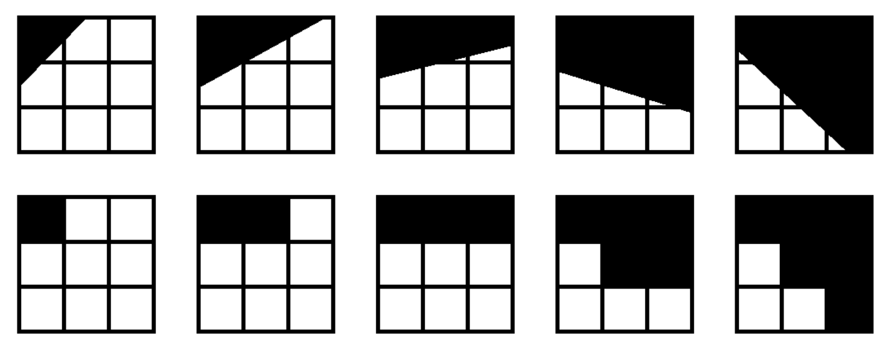
Before describing our results on optical flow patches, we first describe the nonlinear statistics of range image patches (which contain a distance at each pixel), which will play an important role in the theory behind our results. [31] observes that high-contrast $3\times 3$ range patches from [29] cluster near binary patches. [3] uses persistent homology to find that the densest range clusters are arranged in the shape of a circle. After enlarging to $5\times 5$ or $7\times 7$ patches, the entire primary circle in Figure 4(a) is dense. The patches forming the range primary circle are binary approximations to linear step edges; see Figure 4(b).

We explore the nonlinear statistics of high-contrast $3\times 3$ optical flow patches from the computer-generated video short Sintel using topological machinery, primarily persistent homology and zigzag persistence. Since no instrument can measure ground-truth optical flow, an understanding of the nonlinear statistics of flow is needed in order to serve as a prior for optical flow estimation algorithms. With a global estimate of density, the densest patches lie near a circle, the horizontal flow circle. Upon selecting the optical flow patches whose predominant direction of flow lies in a small bin of angle values, we find that the patches in each such bin are well-modeled by a circle. By combining these bins together we obtain a torus model for optical flow, which furthermore is naturally equipped with the structure of a fiber bundle, over a circular base space of common range image patches.

We thank Gunnar Carlsson, Bradley Nelson, Jose Perea, and Guillermo Sapiro for helpful conversations.

References

- [1] Henry Adams, Atanas Atanasov, and Gunnar Carlsson. Nudged elastic band in topological data analysis. Topological Methods in Nonlinear Analysis, 45(1):247–272, 2015.
- [2] Henry Adams, Johnathan Bush, Brittany Carr, Lara Kassab, and Joshua Mirth. On the nonlinear statistics of optical flow. In International Workshop on Computational Topology in Image Context, pages 151–165. Springer, 2019.
- [3] Henry Adams and Gunnar Carlsson. On the nonlinear statistics of range image patches. SIAM Journal on Imaging Sciences, 2(1):110–117, 2009.
- [4] Henry Adams, Sofya Chepushtanova, Tegan Emerson, Eric Hanson, Michael Kirby, Francis Motta, Rachel Neville, Chris Peterson, Patrick Shipman, and Lori Ziegelmeier. Persistence images: A vector representation of persistent homology. Journal of Machine Learning Research, 18(8):1–35, 2017.
- [5] Mark Anthony Armstrong. Basic Topology. Springer Science & Business Media, 2013.
- [6] Simon Baker, Daniel Scharstein, JP Lewis, Stefan Roth, Michael J Black, and Richard Szeliski. A database and evaluation methodology for optical flow. International Journal of Computer Vision, 92(1):1–31, 2011.
- [7] Wei Bao, Hong Li, Nan Li, and Wei Jiang. A liveness detection method for face recognition based on optical flow field. In Image Analysis and Signal Processing, 2009. IASP 2009. International Conference on, pages 233–236. IEEE, 2009.
- [8] John L Barron, David J Fleet, and Steven S Beauchemin. Performance of optical flow techniques. International Journal of Computer Vision, 12(1):43–77, 1994.
- [9] Yuliy Baryshnikov and Robert Ghrist. Target enumeration via euler characteristic integrals. SIAM Journal on Applied Mathematics, 70(3):825–844, 2009.
- [10] Ulrich Bauer. Ripser: A lean C++ code for the computation of Vietoris–Rips persistence barcodes. Software at https://github.com/Ripser/ripser, 2017.
- [11] Steven S. Beauchemin and John L. Barron. The computation of optical flow. ACM computing surveys (CSUR), 27(3):433–466, 1995.
- [12] Paul Bendich, James S Marron, Ezra Miller, Alex Pieloch, and Sean Skwerer. Persistent homology analysis of brain artery trees. The annals of applied statistics, 10(1):198, 2016.
- [13] Peter Bubenik. Statistical topological data analysis using persistence landscapes. The Journal of Machine Learning Research, 16(1):77–102, 2015.
- [14] Dan Burghelea and Tamal K Dey. Topological persistence for circle-valued maps. Discrete & Computational Geometry, 50(1):69–98, 2013.
- [15] Daniel J Butler, Jonas Wulff, Garrett B Stanley, and Michael J Black. A naturalistic open source movie for optical flow evaluation. In European Conference on Computer Vision, pages 611–625. Springer, 2012.
- [16] Gunnar Carlsson. Topology and data. Bulletin of the American Mathematical Society, 46(2):255–308, 2009.
- [17] Gunnar Carlsson and Vin de Silva. Zigzag persistence. Foundations of Computational Mathematics, 10(4):367–405, 2010.
- [18] Gunnar Carlsson, Vin De Silva, and Dmitriy Morozov. Zigzag persistent homology and real-valued functions. In Proceedings of the twenty-fifth annual symposium on Computational geometry, pages 247–256. ACM, 2009.
- [19] Gunnar Carlsson, Tigran Ishkhanov, Vin De Silva, and Afra Zomorodian. On the local behavior of spaces of natural images. International Journal of Computer Vision, 76(1):1–12, 2008.
- [20] Moo K. Chung, Peter Bubenik, and Peter T. Kim. Persistence diagrams of cortical surface data. In Information Processing in Medical Imaging, pages 386–397. Springer, 2009.
- [21] Vin De Silva and Gunnar Carlsson. Topological estimation using witness complexes. SPBG, 4:157–166, 2004.
- [22] Vin de Silva and Robert Ghrist. Coordinate-free coverage in sensor networks with controlled boundaries via homology. The International Journal of Robotics Research, 25(12):1205–1222, 2006.
- [23] Herbert Edelsbrunner and John L Harer. Computational Topology: An Introduction. American Mathematical Society, Providence, 2010.
- [24] Herbert Edelsbrunner, David Letscher, and Afra Zomorodian. Topological persistence and simplification. In Foundations of Computer Science, 2000. Proceedings. 41st Annual Symposium on, pages 454–463. IEEE, 2000.
- [25] David Fleet and Yair Weiss. Optical flow estimation. In Handbook of Mathematical Models in Computer Vision, pages 237–257. Springer, 2006.
- [26] Andreas Geiger, Philip Lenz, Christoph Stiller, and Raquel Urtasun. Vision meets robotics: The KITTI dataset. International Journal of Robotics Research (IJRR), 2013.
- [27] Allen Hatcher. Algebraic Topology. Cambridge University Press, Cambridge, 2002.
- [28] Berthold KP Horn and Brian G Schunck. Determining optical flow. Artificial intelligence, 17(1-3):185–203, 1981.
- [29] Jinggang Huang, Ann B Lee, and David Bryant Mumford. Statistics of range images. In Proceedings of the IEEE Conference on Computer Vision and Pattern Recognition, pages 324–332, 2000.
- [30] David A Huffman. A method for the construction of minimum-redundancy codes. Proceedings of the IRE, 40(9):1098–1101, 1952.
- [31] Ann B Lee, Kim S Pedersen, and David Mumford. The nonlinear statistics of high-contrast patches in natural images. International Journal of Computer Vision, 54(1-3):83–103, 2003.
- [32] PY Lum, G Singh, A Lehman, T Ishkanov, Mikael Vejdemo-Johansson, M Alagappan, J Carlsson, and G Carlsson. Extracting insights from the shape of complex data using topology. Scientific reports, 3:1236, 2013.
- [33] Oisin Mac Aodha, Ahmad Humayun, Marc Pollefeys, and Gabriel J. Brostow. Learning a confidence measure for optical flow. IEEE Transactions on Pattern Analysis and Machine Intelligence, 35(5):1107–1120, 2013.
- [34] Dmitriy Morozov. Dionysus. http://www.mrzv.org/software/dionysus2/.
- [35] Jose A Perea and Gunnar Carlsson. A Klein-bottle-based dictionary for texture representation. International journal of computer vision, 107(1):75–97, 2014.
- [36] T (Producer) Roosendaal. Sintel. Blender Foundation, Durian Open Movie Project, http://www.sintel.org/, 2010.
- [37] Stefan Roth and Michael J Black. On the spatial statistics of optical flow. International Journal of Computer Vision, 74(1):33–50, 2007.
- [38] Chad M Topaz, Lori Ziegelmeier, and Tom Halverson. Topological data analysis of biological aggregation models. PloS one, 10(5):e0126383, 2015.
- [39] Gregory K Wallace. The JPEG still picture compression standard. IEEE transactions on consumer electronics, 38(1):xviii–xxxiv, 1992.
- [40] Kelin Xia and Guo-Wei Wei. Persistent homology analysis of protein structure, flexibility, and folding. International journal for numerical methods in biomedical engineering, 30(8):814–844, 2014.
- [41] Afra Zomorodian and Gunnar Carlsson. Computing persistent homology. Discrete & Computational Geometry, 33(2):249–274, 2005.