Topological surgery in cosmic phenomena

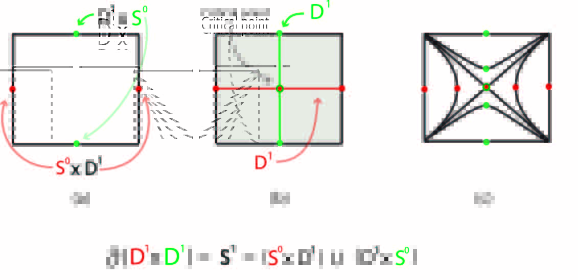
Let us first notice that if we glue together the two $m$-manifolds with boundary involved in the process of $m$-dimensional $n$-surgery, along their common boundary using the standard mapping $h$, we obtain the $m$-sphere which, in turn, is the boundary of the $(m+1)$-dimensional disc: $(S^{n}\times D^{m-n})\cup_{h}(D^{n+1}\times S^{m-n-1})=(\partial D^{n+1}\times D^{m-n})\cup_{h}(D^{n+1}\times\partial D^{m-n})=\partial(D^{n+1}\times D^{m-n})\cong\partial(D^{m+1})=S^{m}$. For example, in dimension 1, $(S^{0}\times D^{1})\cup_{h}(D^{1}\times S^{0})=S^{1}$, see Fig. 2 (a).

The $(m+1)$-dimensional disc $D^{m+1}\cong D^{n+1}\times D^{m-n}$ is one dimension higher than the initial manifold $M^{m}$. This extra dimension leaves room for the process of surgery to take place continuously. The disc $D^{m+1}$ considered in its homeomorphic form $D^{n+1}\times D^{m-n}$ is an $(m+1)$-dimensional $(n+1)$-handle. The unique intersection point $D^{n+1}\cap D^{m-n}$ within $D^{n+1}\times D^{m-n}$ is called the critical point. For example, Fig. 2 (b) illustrates the $2$-dimensional $1$-handle $D^{1}\times D^{1}$ in which $1$-dimensional $0$-surgery takes place and the corresponding critical point.

The process of surgery is the continuous passage, within the handle $D^{n+1}\times D^{m-n}$, from boundary component $(S^{n}\times D^{m-n})\subset\partial(D^{n+1}\times D^{m-n})$ to its complement $(D^{n+1}\times S^{m-n-1})\subset\partial(D^{n+1}\times D^{m-n})$. More precisely, the boundary component $(S^{n}\times D^{m-n})$ collapse to the critical point $D^{n+1}\cap D^{m-n}$ from which the complement boundary component $(D^{n+1}\times S^{m-n-1})$ emerges.

For the case of $1$-dimensional $0$-surgery, this local process within the handle $D^{1}\times D^{1}$ is shown in Fig. 2 (c) where the two segments $S^{0}\times D^{1}$ approach each other, touch at the critical point $D^{1}\cap D^{1}$, where they break, reconnect and become segments $D^{1}\times S^{0}$.

Note that each temporal ‘slice’ of this process is an $m$-dimensional manifold but the evolution of the process requires $m+1$ dimensions in order to be visualized. These local intermediate ‘slices’ will be further analyzed in Section 3.

In order to visualize the global process of surgery which transforms $M$ into $M^{\prime}$, one also requires $m+1$ dimensions. In fact, surgery on the $m$-manifold $M$ determines a cobordism $(W;M,M^{\prime})$ called the surgery trace which is made of the temporal ‘slices’ of the global process. More precisely:

The cobordism $(W;M,M^{\prime})$ of Fig. 3 illustrates these definitions for the case of $1$-dimensional $0$-surgery. The local process is part of the global process, hence one can see the handle $D^{1}\times D^{1}$ of Fig. 2 (b) in Fig. 3. Further, while not explicitly stated so far, the reader might have already seen from Fig. 1 that a $1$-dimensional $0$-surgery on $M=S^{1}$ gives us $M^{\prime}=S^{0}\times S^{1}$. This is also shown in Fig. 3 where we see how the initial manifold $M=S^{1}\times{\{0\}}$ is cobordant with the resulting manifold $M^{\prime}=S^{0}\times S^{1}\times{\{1}\}$, which is shown in Fig. 3 in light green. Hence Fig. 3 shows $(W;M,M^{\prime})=(S^{1}\times I\cup D^{1}\times D^{1};S^{1},S^{0}\times S^{1})$.

However, in order to be able to visualize the temporal ‘slices’ of the global process as perpendicular crossections of the cobordism of Fig. 3, a homeomorphic representation of $W$ is needed. This is shown in Fig. 4, where the local process within handle $D^{1}\times D^{1}$ can be seen as part of the the global process of $1$-dimensional $0$-surgery on $S^{1}$ which, in turn, can be seen as ‘slices’ of $W$.

We will start by recalling two basic definitions:

Morse theory studies differentiable manifolds $M$ by considering the critical points of Morse functions $f:M\to\mathbb{R}$, see [9] for details. Among others, Morse theory is used to prove that an $m$-dimensional manifold $M$ can be obtained from $\emptyset$ by successively attaching handles of increasing index $i$:

The basic connection between Morse theory, cobordisms and topological surgery comes from the following two propositions [8]:

The proof of Proposition 1 (i) and (ii) can be found in [9] and [8] respectively, while for Proposition 2 the reader is referred to [9]. For example, in the case of $1$-dimensional $0$-surgery, since $m=1$ and $n=0$, the single critical point of index $i=1$ mentioned in Proposition 1 (ii) is $D^{1}\cap D^{1}$ which is in the interior of the handle $D^{1}\times D^{1}$, recall Fig. 2 (b). The corresponding cobordism $W$ referred to in Proposition 2 and shown in Figs. 3 and  4, is obtained by attaching the handle $D^{1}\times D^{1}$ to $W_{0}=M\times I=S^{1}\times I$ while $\partial W=S^{1}\sqcup S^{0}\times S^{1}$ is obtained by a $1$-dimensional $0$-surgery on $\partial W_{0}=S^{1}\sqcup S^{1}$.

We will now present a theorem and a lemma from [8] which will be used to study the temporal evolution of topological surgery in the following sections.

For example, the case $m=i=1$ of the lemma is shown in Fig. 5 where:

Lemma 1 connects Morse functions with both the cobordism of the global process and the handle of the local process. Moreover, the local process of $m$-dimensional $(i-1)$-surgery within the $(m+1)$-dimensional handle, recall Fig. 2 (c), can be parametrized by $\epsilon$. Indeed, comparing Fig. 5 with Fig. 2 (c), the values $\epsilon<0$ correspond to the two segments $S^{0}\times D^{1}$ approaching each other, $\epsilon=0$ corresponds to the straighten segments which intersect at the critical point $D^{1}\cap D^{1}$, while the values $\epsilon>0$ correspond to the reconnected segments $D^{1}\times S^{0}$.

As mentioned in the end of Section 3.2, the Morse function for the case $m=i=1$ of Lemma 1 is: $f(x,y)=-x^{2}+y^{2}$. Its plotting is shown in Fig. 6 (1). Now, parameter $\epsilon$ can be considered as time so we shall denote it by $t$. So, we can describe the process of surgery by varying parameter $t$ of the level curves $-x^{2}+y^{2}=t$, illustrated in Fig. 6 (2), thus providing a continuous analogue of the process illustrated in Fig. 5. For $-1<t<0$, these hyperbolas are shaded in red. As $t$ gets close to $0$, the two branches of the hyperbolas get close to one another and their color whitens. At $t=0$ the degenerated hyperbola $-x^{2}+y^{2}=0$ consist in two straight white segments along which the reconnection takes place. Finally, as $t$ starts taking positive values in the range $0<t<1$, the two new branches of the hyperbolas start turning to green.

The gradient vector field $\nabla f=(-2x,2y)$, which is perpendicular to the level curves $-x^{2}+y^{2}=t$ and points in the direction of the greatest rate of increase of $f$, is shown in Fig. 7. The flow of $S^{0}$ which is composed of the two red points $(-1,0)\sqcup(1,0)$ in Fig. 7, follows the red vectors along the $x$-axis towards the critical point $(0,0)$. After collapsing to the critical point, two new green points emerge, following the green vectors along the $y$-axis towards the $S^{0}$ composed of the green points $(0,1)\sqcup(0,-1)$. In other words, the process of $1$-dimensional $0$-surgery can be viewed as the collapsing of the core $S^{0}$ of segments $S^{0}\times D^{1}$ to the critical point from which the core $S^{0}$ of segments $D^{1}\times S^{0}$ uncollapses. The two directions followed by the cores are the two perpendicular segments $D^{1}$ that make up the $2$-dimensional $1$-handle $D^{1}\times D^{1}$. These segments were shown in red and green in Fig. 5 and the same color coding has been used to show the vectors acting along them in Fig. 7.

Moreover, the gradient is closely related to the notion of force. For example, an object starting from a high place (thus having high potential energy) and rolling down to a lower place (of lower potential energy) under the influence of gravity will follow the exact opposite direction of the gradient vectors. Looking at Fig. 6 (1) and letting two small objects fall from the two highest points $(0,1,1)$ and $(0,-1,1)$, these objects will meet at $(0,0,0)$ and fall down to the two lowest points $(1,0,0)$ and $(-1,0,0)$. Their path projected in $2$-dimensions corresponds to the time-reversed process of Fig. 7: two green points $S^{0}$ collapsing to the critical point from which the two red points $S^{0}$ emerge. We can think of the Morse function as describing the height (hence related to the potential energy) and of the objects as rolling down the hills described by the Morse function. The gravitational force and the motion of the objects are both in the direction of the negative gradient of the Morse function, perpendicular to its level curves.

More generally, if the forces acting on a particle are conservative, they are derivable from a scalar potential energy function $V$ as $\vec{F}=-(\nabla V)$. Hence, for phenomena exhibiting such surgery, one can take the local form of the corresponding Morse function multiplied by $-1$: $(-1)*f$ as a potential energy function giving rise to the local forces related to surgery.

The above analysis provides a way to describe natural phenomena exhibiting $1$-dimensional $0$-surgery. Such phenomena occur in both micro and macro scales. It can be seen for example during magnetic reconnection (the phenomenon whereby cosmic magnetic field lines from different magnetic domains are spliced to one another, changing their pattern of conductivity with respect to the sources), during meiosis (when new combinations of genes are produced) and in site-specific DNA recombination (whereby nature alters the genetic code of an organism). These phenomena and their relation to topological surgery have been detailed in [1] where we pin down the forces that are present in each process.

Note that this analysis also gives us an algebraic description of the process. More precisely, we can now use equation $-x^{2}+y^{2}=t,-1<t<1$, to describe the continuous way the $1$-dimensional splicing and reconnection occurs. Moreover, it generalizes the notion of forces to the negative gradient of the local form of the corresponding Morse function. As a result, if we view the gradient vectors of Fig. 7 as forces, these act not only on the cores $S^{0}$ but on the whole segments $S^{0}\times D^{1}$ and $D^{1}\times S^{0}$. Moreover, while the collapse of the core $S^{0}$ of the initial segments $S^{0}\times D^{1}$ is the effect of attracting forces, we now pin down that the uncollapsing of the core $S^{0}$ of the final segments $D^{1}\times S^{0}$ is the result of repelling forces. Note that we will keep this color coding throughout the paper. Namely vectors exhibiting attraction and repulsion will be shown in red and green, respectively.

From Definition 1, we know that there are two types of $2$-dimensional surgery. Namely, starting with a $2$-manifold $M$, one can have $m=2$ and $n=0$ or $m=2$ and $n=1$. The first possibility is the $2$-dimensional $0$-surgery which removes two discs $S^{0}\times D^{2}$ from $M$ and replaces them by a cylinder $D^{1}\times S^{1}$. This cylinder gets attached along the common boundary $S^{0}\times S^{1}$ comprising two copies of $S^{1}$. For example, if $M=S^{2}$ the above operation changes its homeomorphism type from the 2-sphere to that of the torus, see Fig. 8 (a). The other possibility is the $2$-dimensional $1$-surgery where a cylinder (or equivalently an annulus) $S^{1}\times D^{1}$ is removed from $M$ and is replaced by two discs $D^{2}\times S^{0}$ attached along the common boundary $S^{1}\times S^{0}$. For example, if $M=S^{2}$ the result is two copies of $S^{2}$, see Fig. 8 (b).

Note now that from Definition 1, a dual $2$-dimensional $0$-surgery is a $2$-dimensional $1$-surgery and vice versa. Hence, Fig. 8 (a) shows that a $2$-dimensional $0$-surgery on a sphere is the reverse process of a $2$-dimensional $1$-surgery on a torus, while Fig. 8 (b) shows that $2$-dimensional $1$-surgery on a sphere is the reverse process of a $2$-dimensional $0$-surgery on two spheres. In the figure, the symbol $\longleftrightarrow$ indicates surgeries from left to right and their corresponding dual surgeries from right to left.

Consider now the Morse function of Lemma 1 for the case $m=2$ and $i=1$, namely:

Applying the line of thought presented in Section 4 one dimension higher, the local process of $2$-dimensional $0$-surgery happens inside handle $D^{1}\times D^{2}$ and can be described by varying parameter $t$ of the level surfaces $-x^{2}+y^{2}+z^{2}=t$. For $-1<t<0$, these are two-sheet hyperboloids. In Fig. 9, one of these two-sheets hyperboloids is shown intersecting with the $x$-axis at the two antipodal red points. As $t$ gets close to $0$, the two-sheets of the hyperboloids get close to one another. At $t=0$ the two sheets merge and become the conical surface $-x^{2}+y^{2}+z^{2}=0$ centered at $(0,0,0)$, see the red/green point of Fig. 9, from which, as $t$ takes positive values in the range $0<t<1$, the new one-sheet hyperboloids emerge. One of these one-sheet hyperboloids is shown in Fig. 9 where its intersection with the $(y,z)$-plane is the circle shown in green. Similarly, for $2$-dimensional $1$-surgery, one could consider the Morse function of Lemma 1 for the case $m=2$ and $i=2$. However, one can simply reverse the time of the Morse function of $2$-dimensional $0$-surgery, $g(x,y,z)=-x^{2}+y^{2}+z^{2}$, to obtain the level surfaces $-x^{2}+y^{2}+z^{2}=(-t)$, which describe the local process of $2$-dimensional $1$-surgery. In Fig. 9, this process starts from a one-sheet hyperboloid which is continuously transformed to the ending two-sheets hyperboloid.

The gradient vector field $\nabla g=(-2x,2y,2z)$ which is perpendicular to the level surfaces $-x^{2}+y^{2}+z^{2}=t$ describing $2$-dimensional $0$-surgery is shown in Fig. 9. The flow of $S^{0}$, which is composed of the two red points $(-1,0,0)\sqcup(1,0,0)$ in Fig. 9, follows the red vectors along the $x$-axis towards the critical point $(0,0,0)$. After collapsing, the new green circle $S^{1}$ emerges along the $(y,z)$-plane as a result of the green vectors. In other words, the process of $2$-dimensional $0$-surgery can be seen as the collapsing of the core $S^{0}$ of discs $S^{0}\times D^{2}$ to the critical point from which the core $S^{1}$ of cylinder $D^{1}\times S^{1}$ uncollapses. The two directions followed by the cores are along the (red) segment $D^{1}$ on the $(x)$-axis and the (green) disc $D^{2}$ on the $(y,z)$-plane that make up the $3$-dimensional $1$-handle $D^{1}\times D^{2}$ in $\mathbb{R}^{3}$. If we view the gradient vectors of Fig. 9 as forces, the attracting forces acting on the core $S^{0}$ are fleshed out to the whole $S^{0}\times D^{2}$ until the critical point is reached after which, the repelling forces uncollapsing the core $S^{1}$ are fleshed out to the cylinder $D^{1}\times S^{1}$.

Taking the one dimension higher analogue of $1$-dimensional $0$-surgery presented in Section 4.2, if the forces acting on a particle are conservative, then the local form of the Morse function $g$ can be used as a potential energy function giving rise to the local forces related to $2$-dimensional $0$-surgery: $\vec{F}=-(\nabla V)=\nabla g$. The gradient vector field perpendicular to the level surfaces describing $2$-dimensional $1$-surgery can be described analogously.

The above analysis provides a way to describe natural phenomena exhibiting $2$-dimensional surgery, that is, phenomena where $2$-dimensional merging and recoupling occurs. Roughly speaking, $2$-dimensional $0$-surgery can be seen in phenomena where a cylinder is created, while $2$-dimensional $1$-surgery can be seen in phenomena where a cylinder is collapsed.

Examples of $2$-dimensional $0$-surgery comprise the formation of tornadoes, drop coalescence (the phenomenon where two dispersed drops merge into one), gene transfer in bacteria (where the donor cell produces a connecting tube called a ‘pilus’ which attaches to the recipient cell) and the formation of Falaco solitons, see Fig. 10 (1). Each Falaco soliton consists of a pair of locally unstable but globally stabilized contra-rotating identations in the water-air surface of a swimming pool, see [10] for details. The cylinder that is being created can take various forms. For example, it is a tubular vortex of air in the case of tornadoes, a pilus joining the genes during bacterial gene transfer and transverse torsional waves in the case of Falaco solitons, see Fig. 10 (2).

On the other hand, $2$-dimensional $1$-surgery can be seen during soap bubble splitting (where a soap bubble splits into two smaller bubbles), when the tension applied on metal specimens by tensile forces results in the phenomena of necking and then fracture and in the biological process of mitosis (where a cell splits into two new cells). These phenomena are characterized by a ‘necking’ occurring in a cylinder $D^{1}\times S^{1}$, which degenerates into a point and finally tears apart creating two discs $S^{0}\times D^{2}$. The cylinder that is about to collapse can be embedded, for example, in the region of the bubble’s surface where splitting occurs, on the region of metal specimens where necking and fracture occurs, or on the equator of the cell which is about to undergo a mitotic process. These phenomena and their relation to topological surgery have been detailed in [1] where we pin down the forces that are present is these processes.

With this analysis, the local form of the Morse function $g$ can be used to describe algebraically the processes of $2$-dimensional surgeries. Moreover, our analysis provides a novel description of these processes if the gradient vectors $\nabla g$ of Fig. 9 are viewed as forces.

In this section, based on the phenomenon of Falaco solitons creation, we will examine the local process of topological surgery for non-trivial embeddings (recall Definition 1).

Let us start by pointing out that, for phenomena exhibiting $2$-dimensional $0$-surgery, the various forms of the attached cylinder are homeomorphic representations of the cylinder $D^{1}\times S^{1}$ shown in Fig. 9. For example, during the formation of Falaco solitons, the cylinder (and the whole $3$-dimensional $1$-handle $D^{1}\times D^{2}$ inside which the local process takes place) is bended and twisted, see Fig. 10 (2). Note that the singular thread shown in Fig. 10 (1) is the segment $D^{1}$ joining the core $S^{0}$, which in this case comprises the two central points of the Falaco solitons.

Up to now, when referring to the embedding $h$ of Definition 1, we have assumed that the standard (or trivial) embedding, which we will denote by $h_{s}$, was used. For example, the process of $2$-dimensional $0$-surgery shown in Fig. 9 does not involve twisting. The same process is shown in Fig. 11 (1) where the key instances have been discretized for the purpose of clarity. However, many phenomena, including the formation of Falaco solitons, correspond to a non-trivial embedding, say $h_{t}$, which involves twisting. The two indentations of Fig. 10 (1) can be seen as the first instance of the local process of $2$-dimensional $0$-surgery, which can be described by an embedding $h_{t}(S^{0}\times D^{2})$ twisting the two discs. An example of such an embedding can be seen in the leftmost instance of Fig. 11 (2). The cylindrical vortex $D^{1}\times S^{1}$ made from the propagation of the torsional waves around the singular thread seen in Fig. 10 (2) can be considered as the final instance of the process, corresponding to the rightmost instance of Fig. 11 (2).

The difference between the two embeddings $h=h_{s}$ and $h=h_{t}$ is shown in Fig. 11 (1) and (2) respectively. More precisely, if we consider counterclockwise rotations as positive, embedding $h_{t}$ rotates the two initial discs by $-3\pi/4$ and $3\pi/4$ respectively, see the passage from the leftmost instance of Fig. 11 (1) to the leftmost instance of Fig. 11 (2). If we define the homeomorphisms $\omega_{1},\omega_{2}:D^{2}\to D^{2}$ to be rotations by $-3\pi/4$ and $3\pi/4$ respectively, then $h_{t}$ is defined as the composition $h_{t}:S^{0}\times D^{2}\xrightarrow{\omega_{1}\amalg\omega_{2}}S^{0}\times D^{2}\xrightarrow{h}M$. This rotation induces the twisting $g_{t}$ of angle $-3\pi/2$ of the final cylinder, see the rightmost instances of Fig. 11 (1) and (2).

When the topological thread is cut, for example when the Falaco solitons hit an obstacle perpendicular to their displacement, the cylindrical vortex tears apart and slowly degenerates to the two discs until they both stop spinning and vanish. Note that since the dissipation of Falaco solitons is slower than their creation, the intermediate instances of this process can be visualized in real time in experiments such as [11]. This reverse process is the passage from Fig. 10 (2) to Fig. 10 (1) and corresponds to the $2$-dimensional $1$-surgery shown from right to left in Fig. 11 (2).

In this case, the initial cylinder is twisted. In our example, homemorphism $g_{t}$ rotates the top and bottom of the cylinder by $-3\pi/4$ and $3\pi/4$ respectively, see the passage from the rightmost instance of Fig. 11 (1) to the rightmost instance of Fig. 11 (2). This rotation induces the twisting of the two final discs, as in the leftmost instance of Fig. 11 (2).

Let us finally conclude that the homeomorphisms $h_{t}$ and $g_{t}$ as illustrated in Fig. 11 provide a better description of the creation (or dissipation) of Falaco solitons and, more generally, of phenomena involving twisting with ‘drilling’ (or twisting with ‘necking’).

From Definition 1, we know that there are three types of surgery in dimension $3$. Namely, starting with a 3-manifold $M$, for $m=3$ and $n=0$, we have the $3$-dimensional $0$-surgery, whereby two 3-balls $S^{0}\times D^{3}$ are removed from $M$ and are replaced in the closure of the remaining manifold by a thickened sphere $D^{1}\times S^{2}$:

$\chi(M)=\overline{M\setminus h(S^{0}\times D^{3})}\cup_{h}(D^{1}\times S^{2})$

Next, for $m=3$ and $n=2$, we have the $3$-dimensional $2$-surgery, which is the reverse (dual) process of $3$-dimensional $0$-surgery.

Finally, for $m=3$ and $n=1$, we have the $3$-dimensional $1$-surgery, whereby a solid torus $S^{1}\times D^{2}$ is removed from $M$ and is replaced by another solid torus $D^{2}\times S^{1}$ (with the factors now reversed) via a homeomorphism $h$ of the common boundary:

$\chi(M)=\overline{M\setminus h(S^{1}\times D^{2})}\cup_{h}(D^{2}\times S^{1})$

This type of surgery is clearly self-dual.

Consider the Morse function of Lemma 1 for the case $m=3$ and $i=1$:

Applying the line of thought presented in Sections 4 and 5, the local process of $3$-dimensional $0$-surgery happens inside the $4$-dimensional handle $D^{1}\times D^{3}$ and can be described by varying parameter $t$ of the level hypersurfaces $-x^{2}+y^{2}+z^{2}+w^{2}=t$. These hypersufaces and the perpendicular gradient vector field $\nabla f=(-2x,2y,2z,2w)$ require four dimensions in order to be visualized. However, we can describe and visualize the behaviors of the cores and the gradient along their direction of movement. We will refer to this visualization as the ‘core view’ of $3$-dimensional $0$-surgery. The process starts with the core $S^{0}$ of $S^{0}\times D^{3}$, see the two red points in the leftmost instance of Fig. 12 (1). These two points are attracted towards $(0,0,0,0)$ under the influence of the gradient $\nabla f=(-2x,2y,2z,2w)$ which is negative along the horizontal axis $x$. Along $x$, the local form of the corresponding Morse function is $-x^{2}=t$ for $-1<t<0$. The two points touch at the critical point $(0,0,0,0)$ which is the intersection $D^{1}\cap D^{3}$ (within the $4$-dimensional handle $D^{1}\times D^{3}$), see the middle instance of Fig. 12 (1). Then, the core $S^{2}$ of $D^{1}\times S^{2}$ uncollapses along the axes $y,z,w$ under the influence of the gradient $\nabla f=(-2x,2y,2z,2w)$ which is positive along axes $y,z,w$, see the rightmost instance of Fig. 12 (1). The local form of the corresponding Morse function along $y,z,w$ is $w^{2}+z^{2}+y^{2}=t$ for $0<t<1$. Note that the core $S^{0}$ (respectively the core $S^{2}$) bounds the disc $D^{1}$ (respectively the $3$-ball $D^{3}$) of the $4$-dimensional handle $D^{1}\times D^{3}$ in which the process takes place. If we view the gradient of Fig. 12 (1) as a force, one can imagine the $4$-dimensional process by following the line of thought presented in Section 5.3. Namely, the attracting forces acting on the cores $S^{0}$ are fleshed out to the two $3$-balls $S^{0}\times D^{3}$ until the critical point is reached, after which the repelling forces uncollapsing the core $S^{2}$ are fleshed out to the thickened sphere $D^{1}\times S^{2}$.

Similarly, for $3$-dimensional $1$-surgery, we consider the Morse function of Lemma 1 for the case $m=3$ and $i=2$:

In this case, the local process of $3$-dimensional $1$-surgery happens inside the handle $D^{2}\times D^{2}$ and can be described by varying parameter $t$ of the level hypersurfaces $-x^{2}-y^{2}+z^{2}+w^{2}=t$. In Fig. 12 (2), the ‘core view’ of $3$-dimensional $1$-surgery is presented. The process starts with the core $S^{1}$ (shown in red) of the solid torus $S^{1}\times D^{2}$. The points of this circle are attracted towards $(0,0,0,0)$ under the influence of the gradient $\nabla g=(-2x,-2y,2z,2w)$ which is negative along axes $x,y$, see the leftmost instance of Fig. 12 (2). Along these axes, the local form of the corresponding Morse function is $-x^{2}-y^{2}=t$ for $-1<t<0$. The circle collapses at the critical point $(0,0,0,0)=D^{2}\cap D^{2}$, see the middle instance of Fig. 12 (2). Then, the core $S^{1}$ (shown in green in the rightmost instance of Fig. 12 (2)) of the solid torus with the factors reversed, $D^{2}\times S^{1}$, uncollapses along axes $z,w$ under the influence of the gradient $\nabla g=(-2x,-2y,2z,2w)$ which is positive along axes $z,w$. The local from of the corresponding Morse function along $z,w$ is $z^{2}+w^{2}=t$ for $0<t<1$. Note that each core $S^{1}$ bounds a disc $D^{2}$ of the $4$-dimensional handle $D^{2}\times D^{2}$ in which the process takes place. If we view the gradient of Fig. 12 (2) as a force, the $4$-dimensional process can be imagined as follows: the attracting forces acting on the core $S^{1}$ are fleshed out to the solid torus $S^{1}\times D^{2}$ until the critical point is reached, after which the repelling forces uncollapsing the other core $S^{1}$ are fleshed out to the other solid torus $D^{2}\times S^{1}$.

In [2], it is was remarked that $2$-dimensional surgery can be obtained from $1$-dimensional surgery by rotation. Here, we will prove this fact using Morse functions. Let us start by remarking that the level surfaces of $2$-dimensional surgery can be obtained by rotating the level curves of $1$-dimensional $0$-surgery. Indeed, for any given time $t\in(0,1)$, rotating the hyperbolas $-x^{2}+y^{2}=t$ around the $x$-axis creates the surfaces $-x^{2}+y^{2}+z^{2}=t$ which describe $2$-dimensional $0$-surgery, see passage of Fig. 7 to Fig. 9. Note that, instead of rotating each such temporal slice, one can rotate the whole handle which is comprised of them. For example, rotating the handle $D^{1}\times D^{1}$ made of the parametrized hyperbolas of $1$-dimensional $0$-surgery gives us the handle $D^{1}\times D^{2}$ made of the parametrized surfaces of $2$-dimensional $0$-surgery. The rotation happens around the $x$-axis in the $(y,z)$-plane thus turning $D^{1}\times D^{1}$ to $D^{1}\times D^{2}$ by creating the new repelling direction in the $z$-axis, see the passage from Fig. 13 (1) to (2). As also shown in Fig. 13 (1) to (2), the collapsing segments $S^{0}\times D^{1}$ are expanded to $S^{0}\times D^{2}$ while the rotation of core $S^{0}$ of the uncollapsing segments $D^{1}\times S^{0}$ turns into core $S^{1}$ of the uncollapsing cylinder $D^{1}\times S^{1}$. Note that the reverse process of Fig. 13 (2) results in a necking of the cylinder $D^{1}\times S^{1}$, collapsing to the center and recoupling, thus, it describes, $2$-dimensional $1$-surgery via rotation.

Moving one dimension up, the instances of both types of $3$-dimensional surgery can be seen as rotations of the instances of $2$-dimensional $0$-surgery taking place in $D^{1}\times D^{2}$. More precisely, for $3$-dimensional $0$-surgery, a rotation of $D^{1}\times D^{2}$ around the $x$-axis in the $(y,z,w)$-hyperplane turns it to $D^{1}\times D^{3}$ by creating the new repelling direction in the $w$-axis, see Fig. 13 (3). The resulting handle $D^{1}\times D^{3}$ is made of the layering of the hypersurfaces $-x^{2}+y^{2}+z^{2}+w^{2}=t$, $-1<t<1$. In this case, the collapsing discs $S^{0}\times D^{2}$ are thickened to collapsing $3$-balls $S^{0}\times D^{3}$ while the core $S^{1}$ of the uncollapsing cylinder $D^{1}\times S^{1}$ turns into the core $S^{2}$ of the uncollapsing thickened sphere $D^{1}\times S^{2}$, see the passage from Fig. 13 (2) to (3). Note that as handle $D^{1}\times D^{3}$ is $4$-dimensional, only the core view is shown in Fig. 13 (3).

Similarly, for $3$-dimensional $1$-surgery, a rotation around the $y$-axis in the $(x,z,w)$-hyperplane turns $D^{1}\times D^{2}$ to $D^{2}\times D^{2}$ by creating the new attracting direction in the $w$-axis, see Fig. 13 (4). In this case, the resulting handle $D^{2}\times D^{2}$ is made of the hypersurfaces $-x^{2}+y^{2}+z^{2}-w^{2}=t$, $-1<t<1$. Here, the rotation of the core $S^{0}$ of the collapsing discs $S^{0}\times D^{2}$ creates the core $S^{1}$ of the collapsing solid torus $S^{1}\times D^{2}$, while the uncollapsing of the cylinder $D^{1}\times S^{1}$ creates via rotation the uncollapsing solid torus $D^{2}\times S^{1}$, see the passage from Fig. 13 (2) to (4) where only the core view is shown. Note that, in the local form of the Morse function presented here, directions $y$ and $w$ are interchanged compared to the Morse function $g$ presented in the previous section. This is just a matter of convention and is due to the fact that, in Lemma 1, Morse functions sum up the negative coordinates first, hence considering that directions $x$ and $y$ are attracting, whereas here the two attracting directions are $x$ and $w$ because we rotated the predefined coordinates of the local form of the Morse function of $2$-dimensional $0$-surgery.

In the previous section we showed how one can obtain the instances of surgery and the local forms of the corresponding Morse functions for dimensions $1,2$ and $3$. In this section we generalize this idea for an arbitrary surgery dimension $m$.

The local process of an $m$-dimensional $n$-surgery is abstracted in Fig. 14. Its instances are made of hypersurfaces given by:

By varying parameter $t$, one continuously collapses the core $S^{n}$ of the thickened sphere $S^{n}\times D^{m-n}$ to the critical point $D^{n+1}\cap D^{m-n}$ from which the core $S^{m-n-1}$ of the thickened sphere $D^{n+1}\times S^{m-n-1}$ uncollapses. The handle $D^{n+1}\times D^{m-n}$ made of these instances can be obtained by $(m-1)$ successive rotations in increasingly higher dimensions of the initial handle $D^{1}\times D^{1}$ made of the instances of $1$-dimensional $0$-surgery.

One can provide an outline of the $4$-dimensional process of $3$-dimensional surgery by analogy to what happens in one dimension lower. We start by illustrating in Fig. 15 (1) the $3$-dimensional process of $2$-dimensional $0$-surgery. In the figure we deliberately choose a homeomorphic representation, as the one exhibited by Falaco solitons in Fig. 10, where the two discs $S^{0}\times D^{2}$ start embedded in the plane $\mathbb{R}^{2}$, see instance (a) of Fig. 15 (1), but the rest of the process happens in $\mathbb{R}^{3}$, see instances (b)-(e) of Fig. 15 (1).

In analogy, if a $3$-dimensional $0$-surgery starts with two $3$-balls $S^{0}\times D^{3}$ embedded in $\mathbb{R}^{3}$, see instance (a) of Fig. 15 (2), then the rest of the process takes place in $\mathbb{R}^{4}$, see instances (b)-(e) of Fig. 15 (2). Instances (b) and (c) of Fig. 15 (2) illustrate the fact that the two $3$-balls $S^{0}\times D^{3}$ ‘bend’ and touch in the fourth dimension while instances (d) and (e) of the same figure illustrate the emerging of the thickened sphere $D^{1}\times S^{2}$. Note that instances (b)-(e) are deliberately shown with increased transparency to depict the fact that the higher dimensional merging and recoupling is not visible in $\mathbb{R}^{3}$.

Similarly, if a $3$-dimensional $1$-surgery starts with a solid torus $S^{1}\times D^{2}$ embedded in $\mathbb{R}^{3}$, see instance (a) of Fig. 15 (3), then the rest of the process in $\mathbb{R}^{4}$ is outlined in instances (b)-(e) of the same figure. More precisely, instances (b) and (c) sketch the higher dimensional collapse of the solid torus $S^{1}\times D^{2}$ while instances (d) and (e) of Fig. 15 (3) sketch the emerging of the solid torus $D^{2}\times S^{1}$ (with the factors reversed).

References

- 1. Lambropoulou S., Samardzija N., Diamantis I., Antoniou S.: Topological Surgery and Dynamics, Mathematisches Forschungsinstitut Oberwolfach Report No. 26/2014, Workshop: Algebraic Structures in Low-Dimensional Topology. DOI: 10.4171/OWR/2014/26 (2014).
- 2. Antoniou S., Lambropoulou S.: Extending Topological Surgery to Natural Processes and Dynamical Systems. PLOS ONE 12(9). DOI: 10.1371/journal.pone.0183993 (2017).
- 3. Lambropoulou S., Antoniou S.: Topological Surgery, Dynamics and Applications to Natural Processes. Journal of Knot Theory and its Ramifications 26(9). DOI: 10.1142/S0218216517430027 (2016).
- 4. Antoniou S., Lambropoulou S.: Topological Surgery in Nature. Book ‘Algebraic Modeling of Topological and Computational Structures and Applications’, Springer Proceedings in Mathematics and Statistics Vol. 219, DOI: 10.1007/978-3-319-68103-0 (2017).
- 5. Antoniou S.: Mathematical Modeling Through Topological Surgery and Applications. Springer Theses Book Series. Springer International Publishing. DOI: 10.1007/978-3-319-97067-7 (2018).
- 6. Wallace A.H.: Modifications and cobounding manifolds. Canad. J. Math. 12, 503-528 (1960).
- 7. Milnor J.: A procedure for killing the homotopy groups of differentiable manifolds. Symposia in Pure Math., Amer. Math. Soc. 3, 39-55 (1961).
- 8. Ranicki A.: Algebraic and Geometric Surgery. Oxford Mathematical Monographs, Clarendon Press (2002).
- 9. Milnor J.: Morse Theory. Princeton University Press (1963).
- 10. Kiehn R.M.: Non-equilibrium systems and irreversible processes - Adventures in applied topology vol. 1 - Non equilibrium thermodynamics, pp. 147, 150 University of Houston Copyright CSDC Inc (2013).
- 11. Cowern D.: Fun with Vortex Rings in the Pool. Available from:https://www.youtube.com/watch?v=72LWr7BU8Ao.
- 12. Rolfsen D.: Knots and links. Publish or Perish Inc. AMS Chelsea Publishing (2003).
- 13. Munkres J.R.: Topology, Second Edition. Prentice Hall, Incorporated (2000).
- 14. Lickorish W.B.R.: A representation of orientable combinatorial 3-manifolds, Ann. of Math. (2) 76, pp. 531-540 (1962).
- 15. Prasolov V.V., Sossinsky, A.B.: Knots, links, braids and 3-manifolds. AMS Translations of Mathematical Monographs 154 (1997).
- 16. Kirby R.C.: A calculus for framed links in . Invent. Math., 45, pp. 35-56 (1978).
- 17. Kauffman L.H., Lambropoulou S., Buck D.: DNA Topology. (book in preparation). Chapter on ‘Three Dimensional Topology for DNA’.
- 18. Stathis A., Kauffman L.H., Lambropoulou S.: Black holes and topological surgery. Preprint (2018). Available from: https://arxiv.org/pdf/1808.00254.
- 19. Maldacena J., Susskind L.: Cool horizons for entangled black holes. Fortsch.Phys. 61, 781-811. DOI: 10.1002/prop.201300020 (2013). Available from: https://arxiv.org/abs/1306.0533.
- 20. Susskind L.: Copenhagen vs Everett, Teleportation, and ER=EPR. Fortschr. Phys. 64, No. 6–7, 551–564. DOI: 10.1002/prop.201600036 (2016).
- 21. Einstein A., Rosen N.: The particle problem in the general theory of relativity, Phys. Rev. 48, 73-77 (1935).
- 22. Misner C.W., Wheeler J.A.: Classical physics as geometry. Ann. Phys. 2: 525 (1957).
- 23. Collas P., Klein D.: Embeddings and time evolution of the Schwarzschild wormhole, American Journal of Physics 80, 203. DOI: 10.1119/1.3672848 (2012).
- 24. James O., Tunzelmann E., Franklin P., Thorne K.S.: Visualizing Interstellar’s Wormhole. American Journal of Physics 83, 486. DOI:/10.1119/1.4916949 (2015).
- 25. Kiehn R.M.: Falaco Solitons, Cosmic Strings in a Swimming Pool. Preprint (2001). Available from: http://arxiv.org/pdf/gr-qc/0101098v1.
- 26. Thorne K.S.: Black Holes & Time Warps: Einstein’s Outrageous Legacy, W.W. Norton & Company (1994).
- 27. Wheeler J.A.: On the Nature of Quantum Geometrodynamics, Annals Phys. 2, 604-614. DOI: 10.1016/0003-4916(57)90050-7 (1957).
- 28. Baez J.C., Vicary J.: Wormholes and Entanglement. Classical and Quantum Gravity 31. DOI: 10.1088/0264-9381/31/21/214007 (2014). Available from: https://arxiv.org/abs/1401.3416.
- 29. Kauffman L.H., Mehrotra E.: Topological Aspects of Quantum Entanglement (2016). Available from: https://arxiv.org/abs/1611.08047.
- 30. Witten E.: Quantum Field Theory and the Jones Polynomial. Comm. in Math. Phys. Vol. 121, 351-399 (1989).
- 31. Kibble T.W.B.: Topology of cosmic domains and strings. J. Phys. A: Math. Gen., Vol. 9, No. 8: 1387. DOI:10.1088/0305-4470/9/8/029 (1976).
- 32. Hawking S.W.: Black Holes from cosmic strings, Physics Letters B 231 No. 237 DOI: 10.1016/0370-2693(89)90206-2 (1989).
- 33. Caldwell R.R., Casper P.: Formation of Black Holes from Collapsed Cosmic String Loops, Phys.Rev. D53. DOI: 10.1103/PhysRevD.53.3002 (1996).
- 34. MacGibbon J.H., Brandenberger R.H., Wichoski U.F.: Limits on Black Hole Formation from Cosmic String Loops, Phys.Rev. D57 -1998 2158-2165. DOI: 10.1103/PhysRevD.57.2158 (1998).
- 35. Weeks J.R.: The Shape of Space. CRC Press (2001).
- 36. Luminet J.-P., Weeks J.R, Riazuelo A., Lehoucq R.,Uzan J.-P.: Dodecahedral space topology as an explanation for weak wide-angle temperature correlations in the cosmic microwave background. Nature 425, 593–595 (2003).
- 37. Levin J.: Topology and the Cosmic Microwave Background. Physics Reports 365, 251–333 (2002).
- 38. Luminet J.-P.: The Status of Cosmic Topology after Planck Data. Preprint (2016). Available from: https://arxiv.org/abs/1601.03884.
- 39. Adams C.: The Knot Book, An Elementary Introduction to the Mathematical Theory of Knots. American Mathematical Society (2004).
- 40. Rolfsen D.: Knots and links. Publish or Perish Inc. AMS Chelsea Publishing (2003).
- 41. Stillwell J.: Classical Topology and Combinatorial Group Theory. Graduate Texts in Mathematics, Springer-Verlag New York (1993).
- 42. Wilhelm M., Karrass A., Solitar D.: Combinatorial Group Theory, New York: Dover Publications (2004).
- 43. Milnor J.: On the 3-dimensional Brieskorn manifolds M(p,q,r). Knot Groups and 3-Manifolds - Papers dedicated to the memory of R.H.Fox. Annals of Mathematics Studies 84. Princeton University Press, Princeton, NJ (1975).
- 44. Threlfall H., Seifert W. : A textbook of topology. Academic Press (1980).
- 45. Kirby R.C., Scharlemann M.G.: Eight faces of the Poincaré homology 3-sphere. Uspekhi Matematicheskikh Nauk, [N. S.]. DOI: 10.1016/B978-0-12-158860-1.50015-0 (1979).