On the amplitudes for the CP-conserving $\boldsymbol{K^{\pm}(K_{S})\to\pi^{\pm}(\pi^{0})\ell^{+}\ell^{-}}$ rare decay modes

Giancarlo D’Ambrosio Email: gdambros@na.infn.it Affiliation: INFN-Sezione di Napoli, Via Cintia, I-80126 Napoli, Italia David Greynat Email: david.greynat@gmail.com Affiliation: No affiliation and Marc Knecht Email: knecht@cpt.univ-mrs.fr Affiliation: Centre de Physique Théorique, CNRS/Aix-Marseille Univ./Univ. du Sud Toulon-Var (UMR 7332)
CNRS-Luminy Case 907, F-13288 Marseille Cedex 9, France

August 11, 2026

Abstract

The amplitudes for the rare decay modes $K^{\pm}\to\pi^{\pm}\ell^{+}\ell^{-}$ and $K_{S}\to\pi^{0}\ell^{+}\ell^{-}$ are studied with the aim of obtaining predictions for them, such as to enable the possibility to search for violations of lepton-flavour universality in the kaon sector. The issue is first addressed from the perspective of the low-energy expansion, and a two-loop representation of the corresponding form factors is constructed, leaving as unknown quantities their values and slopes at vanishing momentum transfer. In a second step a phenomenological determination of the latter is proposed. It consists of the contribution of the resonant two-pion state in the $P$ wave, and of the leading short-distance contribution determined by the operator-product expansion. The interpolation between the two energy regimes is described by an infinite tower of zero-width resonances matching the QCD short-distance behaviour. Finally, perspectives for future improvements in the theoretical understanding of these amplitudes are discussed.

1 Introduction

Rare kaon decays have been playing a crucial role in flavour physics, and more generally in particle physics. Since they proceed through strangeness-changing neutral currents, they are quite suppressed in the standard model (SM), and thus offer a window through which we might possibly catch a glimpse of new physics (NP). This research subject has been thoroughly reviewed in ref. Cirigliano:2011ny, where a detailed list of references can be found. It is again becoming quite timely nowadays, thanks to experiments like NA62 at the CERN SPS, planning to collect, already in 2018, the data required in order to measure the decay rate of $K^{+}\to\pi^{+}\nu\overline{\nu}$ with a precision of 10 % of its SM prediction Ceccucci:2018bnw; Ceccucci:2018lpb, and KOTO at J-PARC, aiming at measuring the decay rate of $K_{L}\to\pi^{0}\nu\overline{\nu}$ , at around the SM sensitivity in a first stage Komatsubara:2012pn; Shiomi:2014sfa; KOTO.

The study of these rare decay modes of the kaon is of particular interest in view of the present situation in particle physics. Indeed, while no direct evidence for physics beyond the SM was found during the first run of the LHC, there are some interesting indirect hints for NP in the flavour sector, mainly from neutral-current decays of the $B$ meson into di-lepton channels. Here, the very recent result on the $R(K^{*})$ ratio measured by LHCb Aaij:2017vbb has confirmed the deviations from $\mu/e$ universality in neutral currents of the $b\to s\ell^{+}\ell^{-}$ type, $\ell=e,\mu$ , already observed previously in $B\to K\ell^{+}\ell^{-}$ decays Aaij:2014ora,

R(K)=\frac{\text{Br}[B\to K\mu^{+}\mu^{-}]}{\text{Br}[B\to Ke^{+}e^{-}]}=0.745^{+0.090}_{-0.074}\pm 0.036.

(1.1)

This result disagrees with the theoretically clean SM prediction $R_{\rm SM}(K)=1.0003\pm 0.0001$ Bobeth:2007dw; Bordone:2016gaq by $2.6\sigma$ . Further confirmation of this anomaly also comes from $B\to K^{*}\mu^{+}\mu^{-}$ , where an angular observable called $P_{5}^{\prime}$ Descotes-Genon:2013vna, deviates from its SM value with a significance of $2$ – $3\sigma$ , depending on the way hadronic uncertainties are evaluated Descotes-Genon:2013wba; Descotes-Genon:2014uoa; Altmannshofer:2014rta; Jager:2014rwa. Typical NP explanations for the measured $B\to K^{*}\mu^{+}\mu^{-}$ observables require, for instance, $Z^{\prime}$ vector bosons Sierra:2014nqa; Heeck:2014qea; Gauld:2013qba; Buras:2013qja; Gauld:2013qja; Buras:2013dea; Altmannshofer:2014cfa; Glashow:2014iga; Crivellin:2015mga; Dorsner:2015mja; Omura:2015nja; Varzielas:2015joa; Crivellin:2015lwa; Niehoff:2015bfa; Sierra:2015fma; Crivellin:2015era; Celis:2015ara; Carmona:2015ena or leptoquarks Sakaki:2013bfa; Gripaios:2014tna; Becirevic:2015asa; Varzielas:2015iva; Alonso:2015sja; Calibbi:2015kma; Bauer:2015knc; Barbieri:2015yvd; Fajfer:2015ycq; Greljo:2015mma, in order to generate non-SM contributions to current-current effective interactions like $(\bar{s}\gamma_{\alpha}P_{L}b)(\bar{\mu}\gamma^{\alpha}\mu)$ .

The rare processes $K^{\pm}\to\pi^{\pm}\ell^{+}\ell^{-}$ and $K_{S}\to\pi^{0}\ell^{+}\ell^{-}$ are analogous to those mentioned in eq. (1.1), and appear thus as particularly suitable in order to uncover possible violations of lepton-flavour universality (LFUV) in the kaon sector Crivellin:2016vjc. The experimental programs of NA62 NA62_physics (for charged kaon decays) and of LHCb Bediaga:2018lhg; Junior:2018odx (for $K_{S}$ decays) offer quite interesting prospects in this regard. Trying, in parallel, to improve our theoretical understanding of these processes therefore constitutes a quite timely undertaking. It is thus not surprising that efforts in this directions have also become part of the agenda of the lattice-QCD community Isidori:2005tv; Christ:2015aha; Christ:2016mmq.

From the experimental point of view, the situation has evolved in a rather spectacular manner during the last two decades [the present situation is briefly summarized in table 1], especially as far as the two $K^{\pm}\to\pi^{\pm}\ell^{+}\ell^{-}$ channels, where the branching fractions are largest, are concerned. These branching fractions have been measured in refs. Alliegro:1992pp; Adler:1997zk; Ma:1999uj; Park:2001cv and the decays have subsequently been studied more precisely with high statistics in refs. Appel:1999yq; Batley:2009aa; Batley:2011zz, these more recent experiments providing also detailed information on the decay distribution. The latest PDG averages for the branching fractions are Olive:2016xmw

	$\displaystyle\text{Br}[K^{+}\to\pi^{+}e^{+}e^{-}]$	$\displaystyle=(3.00\pm 0.09)\times 10^{-7},$
	$\displaystyle\text{Br}[K^{+}\to\pi^{+}\mu^{+}\mu^{-}]$	$\displaystyle=(9.4\pm 0.6)\times 10^{-8},$		(1.2)

where the error on the muonic mode includes a scale factor $S=2.6$ due to the conflict with the result reported upon in ref. Adler:1997zk. These values lead to $R_{K^{\pm}}[{\rm PDG}]=0.313(71)$ , where

R_{K^{\pm}}\equiv\frac{{\rm Br}[K^{\pm}\to\pi^{\pm}\mu^{+}\mu^{-}]}{{\rm Br}[K^{\pm}\to\pi^{\pm}e^{+}e^{-}]}.

(1.3)

Taking only the high-precision data collected by the NA48/2 Collaboration Batley:2009aa; Batley:2011zz into account, one obtains instead the almost two times more accurate result $R_{K^{\pm}}[{\rm NA48/2}]=0.309(43)$ . In the neutral-kaon sector, the observed decay rates are Batley:2003mu; Batley:2004wg

	$\displaystyle\text{Br}[K_{S}\to\pi^{0}e^{+}e^{-}]_{m_{ee}>0.165\,\text{GeV}}$	$\displaystyle=[3.0^{+1.5}_{-1.2}({\rm stat})\pm 0.2({\rm syst})]\times 10^{-9},$
	$\displaystyle\text{Br}[K_{S}\to\pi^{0}\mu^{+}\mu^{-}]$	$\displaystyle=[2.9^{+1.5}_{-1.2}({\rm stat})\pm 0.2({\rm syst})]\times 10^{-9}.$		(1.4)

These measurements have not yet reached the level of precision already available in the case of the charged kaon.

exp.	ref.	mode	number of events
BNL^∗	Alliegro:1992pp	$K^{+}\to\pi^{+}e^{+}e^{-}$	$\sim 500$
BNL-E865^∗	Appel:1999yq	$K^{+}\to\pi^{+}e^{+}e^{-}$	$10\,300$
NA48/2^∗	Batley:2009aa	$K^{\pm}\to\pi^{\pm}e^{+}e^{-}$	$7\,263$
BNL-E787	Adler:1997zk	$K^{+}\to\pi^{+}\mu^{+}\mu^{-}$	$\sim 200$
BNL-E865	Ma:1999uj	$K^{+}\to\pi^{+}\mu^{+}\mu^{-}$	$\sim 400$
FNAL-E871	Park:2001cv	$K^{\pm}\to\pi^{\pm}\mu^{+}\mu^{-}$	$\sim 100$
NA48/2^∗	Batley:2011zz	$K^{\pm}\to\pi^{\pm}\mu^{+}\mu^{-}$	$3120$
NA48/1	Batley:2003mu	$K_{S}\to\pi^{0}e^{+}e^{-}$	7
NA48/1	Batley:2004wg	$K_{S}\to\pi^{0}\mu^{+}\mu^{-}$	6

Table 1: Experimental situation concerning the decay modes

K^{\pm}\to\pi^{\pm}\ell^{+}\ell^{-}

and

K_{S}\to\pi^{0}\ell^{+}\ell^{-}

. The experiments marked with an asterisk also provide information on the decay distribution.

At the theoretical level, the situation for the CP-conserving decays $K^{\pm}(K_{S})\rightarrow\pi^{\pm}(\pi^{0})\ell^{+}\ell^{-}$ is less favourable than for the $K\to\pi\nu{\bar{\nu}}$ modes. Indeed, whereas the latter are dominated by short distances, the former are governed by the long-distance process $K\to\pi\gamma^{*}\to\pi\ell^{+}\ell^{-}$ EPdR87; EPdR88; DAmbrosio:1998gur, involving a weak form factor, $W_{+}(z)$ in the case of $K^{\pm}\to\pi^{\pm}\gamma^{*}$ , and $W_{S}(z)$ in the case of $K_{S}\to\pi^{0}\gamma^{*}$ . These form factors are given by the matrix elements of the electromagnetic current between a kaon state and a pion state, in the presence of the weak interactions, considered at first order in the Fermi constant. The corresponding momentum transfer squared, the di-lepton invariant mass squared $s=zM_{K}^{2}$ , is small enough, it ranges from $4m_{\ell}^{2}$ to $(M_{K}-M_{\pi})^{2}$ , where $m_{\ell}$ is the mass of the charged lepton, so that these processes can be treated within the framework of chiral perturbation theory (ChPT) Wein79; GassLeut; GassLeut84; Gasser:1984gg. Conservation of the electromagnetic current implies a vanishing contribution at lowest order, ${\mathcal{O}}(E^{2})$ in the chiral expansion. A non-vanishing form factor is generated at next-to-leading order, both by pion and kaon loops, as well as by order ${\mathcal{O}}(E^{4})$ counterterms. The main feature of this one-loop representation of the form factor is the appearance of a unitarity cut on the positive real- $s$ axis, due to the two-pion intermediate state [there is also a cut due to the opening of the $K{\bar{K}}$ channel, but the later is located far enough from the kinematic region of interest, so that its contribution can be, for all practical purposes, approximated by a polynomial]. The corresponding absorptive part (discontinuity) is given by the product of the pion electromagnetic form factor $F_{V}^{\pi}(s)$ with the $P$ -wave projection $f_{1}^{K\pi\to\pi^{+}\pi^{-}}(s)$ of the weak $K\pi\to\pi^{+}\pi^{-}$ amplitude [ $(K,\pi)$ stands for either $(K^{\pm},\pi^{\mp})$ or $(K_{S},\pi^{0})$ ], both taken at tree level. These basic properties of the one-loop form factor already suggest some simple ways to improve upon this result and to collect some ${\mathcal{O}}(E^{6})$ effects. Specifically, in ref. DAmbrosio:1998gur, the $O(E^{2})$ $K\pi\to\pi^{+}\pi^{-}$ vertex was replaced by the phenomenologically well-known Dalitz-plot expansion of the $K\rightarrow\pi\pi^{+}\pi^{-}$ amplitude, and a slope was added to the pion form factor. Furthermore, slopes $b_{+,S}$ in the di-lepton invariant mass squared $s$ , required by the data, but also by order ${\mathcal{O}}(E^{6})$ counterterm contributions, were included in the weak form factors $W_{+,S}(z)$ , in addition to the constant terms $a_{+,S}\propto W_{+,S}(0)$ , already generated by the ${\mathcal{O}}(E^{4})$ counterterms. There are, however, several reasons to go beyond the approximations considered by the authors of ref. DAmbrosio:1998gur:

•

The parameters $a_{+,S}$ and $b_{+,S}$ appear merely as phenomenological constants, which have to be fixed from the available data. We will provide an update of the situation using the most recent data on the decay distributions. At this stage, one may already observe that the value (1.3) obtained for $R_{K^{\pm}}$ is rather different from the one quoted in ref. DAmbrosio:1998gur, $R_{K^{\pm}}=0.167(36)$ , and based on the older data from refs. Adler:1997zk and Alliegro:1992pp. This quite substantial increase in the value of $R_{K^{\pm}}$ confirms the prediction $R_{K^{\pm}}\mathrel{\raise 2.58334pt\hbox{$>$}\kern-7.7778pt\lower 2.79857pt\hbox{$\sim$}}0.23$ made by the authors of ref. DAmbrosio:1998gur. We will also test for potential effects of the data on the value of the curvature (quadratic slope) of the $K^{\pm}\rightarrow\pi^{\pm}\pi^{+}\pi^{-}$ Dalitz plots.
•

Final-state rescattering effects are only partially taken into account by the parameterization of the form factors $W_{+,S}(z)$ proposed in ref. DAmbrosio:1998gur. In particular, the one-loop $P$ -wave projections of the weak $K\pi\to\pi^{+}\pi^{-}$ amplitudes also involve pion rescattering in the crossed channels. Since the two pions are in the $P$ wave, these are not expected to be as large as, for instance, in the case of the $K\to\pi\pi$ amplitudes Cirigliano:2011ny, where the pions are in the $S$ wave. Nevertheless, they could have an impact on the shape of the form factor, and hence on the determinations of $b_{+}$ and $b_{S}$ .
•

The phenomenological values of $a_{+}$ and $b_{+}$ are comparable in size, whereas, from naive chiral counting, one would expect $b_{+}$ to be substantially smaller than $a_{+}$ . A theoretical explanation of $|b_{+}/a_{+}|\sim 1$ is still lacking.
•

Let us close this list with the most important point. The potential detection of any manifestation of LFUV hinges on the possibility to obtain independent information on $a_{+}$ and $b_{+}$ , such as to be able to make a prediction for the ratio $R_{K^{\pm}}$ . This definitely requires to go beyond the low-energy expansion itself.

In order to address these issues, we improve the existing theoretical description of the form factors $W_{+}(z)$ and $W_{S}(z)$ in several ways:

•

We provide complete order ${\mathcal{O}}(E^{6})$ representations of these form factors. They are obtained as the result of a two-step recursive procedure. The first step reproduces the one-loop representations of ref. EPdR87. The second step includes, besides the effects already accounted for by the representation of ref. DAmbrosio:1998gur, all one-loop pion-pion rescattering effects, both in the pion form factor and in the $K\to 3\pi$ vertex.
•

We extend the previous representation of $W_{+}(z)$ beyond the low-energy domain upon using a simple parameterization of the pion form factor that describes the data over a large energy range including the region of the $\rho(770)$ resonance. Since no data are available as far as the $K^{+}\pi^{-}\to\pi^{+}\pi^{-}$ scattering amplitude is concerned [existing data only concern the decay region, in the form of Dalitz-plot expansions], we proceed by applying a unitarization procedure to the ${\mathcal{O}}(E^{4})$ $P$ -wave projection of this amplitude. These two items allow us to construct the absorptive part of the form factor $W_{+}(z)$ arising from two-pion intermediate states. The form factor $W_{+}(z)$ itself is then recovered through an unsubtracted dispersion relation. Upon comparing the behaviour of this “exact” form factor at small values of $z$ with its low-energy expansion, we obtain sum rules for the parameters $a_{+}$ and $b_{+}$ , which we can then compare to their direct determinations from data.
•

We model contributions due to other intermediate states, which occur at higher thresholds, by an infinite sum of single-resonance states, with couplings tuned such as to correctly reproduce the known high-energy behaviour of the form factor in quantum chromo-dynamics (QCD).

For completeness, we should mention that there are other theoretical studies Friot:2004yr; Leskow16; Dubnickova08 of the form factors $W(z)$ that go beyond the low-energy expansion. In ref. Friot:2004yr, a two-parameter representation for $W_{+}(z)$ is proposed, combining the lowest-order chiral expression with resonance exchanges. In ref. Leskow16 the form factors are described within the large- $N_{c}$ treatment of weak hadronic matrix elements, see ref. Buras:1988kp and references quoted therein, matching the quadratic cut-off dependence of the low-energy contribution with the logarithmic one from the short-distance part. Finally, the authors of Dubnickova08 give a representation of the form factors in terms of meson form factors, but the issue of the matching with the short-distance part is not addressed. For a recent account on the theoretical situation of the $K\to\pi\ell^{+}\ell^{-}$ amplitudes, see ref. Portoles:Kaon16.

The content of this paper is consequently organized as follows. In section 2, we first discuss general features of the weak form factors $W_{+,S}(z)$ in QCD, and then address more specifically their short-distance behaviour. Long-distance properties of the form factors are described in section 3, where we recall the results of the existing one-loop calculations EPdR87; AnantIm12, as well as the beyond-one-loop representation of ref. DAmbrosio:1998gur. Phenomenological aspects linked to the determination of $a_{+}$ and $b_{+}$ from the recent high-precision data are the subject of section 4. Starting from a discussion of the analyticity properties of the form factors, we next construct (section 5) a two-loop representation that accounts for all $\pi\pi$ rescattering effects at this order. We compare this representation of the form factors with the one used in ref. DAmbrosio:1998gur, and discuss the impact on the determination of the parameters $a_{+,S}$ and $b_{+,S}$ . Section 6 constitutes the main part of the paper as far as the issues raised above are concerned. There, we construct a dispersive model for the form factor $W_{+}(z)$ . The corresponding absorptive part includes the contribution, now not restricted to low energies, of the $\pi\pi$ intermediate states, and an infinite sum over zero-width resonances, with couplings chosen such as to provide matching with the short-distance behaviour established previously in section 2. Assuming unsubtracted dispersion relations, we evaluate the parameters $a_{+}$ and $b_{+}$ through the corresponding sum rules. A final section summarizes our results and provides our conclusions, as well as critical comments and some perspectives for the future. Numerical values for various input parameters are collected in appendix A. Technical details related to the content of Sec. 5 are displayed in appendix B.

2 Theory overview

In this section, we provide background material concerning the theoretical aspects of the amplitudes describing the weak $K\pi\to\ell^{+}\ell^{-}$ transitions in the standard model, which will also allow us to set up the notation to be used in this study. We first start with the description within the effective four-fermion effective theory below the electroweak scale, and turn next to the short-distance behaviour of the form factors in three-flavour QCD.

2.1 The structure of the form factors in three-flavour QCD

In the standard model, weak non-leptonic ${\Delta S=1}$ transitions of hadrons are described, at a low-energy scale, i.e. below the charm threshold, and at first order in the Fermi constant $G_{F}$ , by an effective lagrangian ${\cal L}_{\Delta S=1}(x)$ given by Gaillard:1974nj; Altarelli:1974exa; Witten:1976kx; Shifman:1975tn; Wise:1979at; Gilman:1979bc

{\cal L}_{\Delta S=1}(x)=-\frac{G_{F}}{\sqrt{2}}V_{us}^{*}V_{ud}\sum_{I=1}^{6}C_{I}(\nu)Q_{I}(x;\nu).

(2.1)

This expression involves the current-current four-quark operators $Q_{1}$ and $Q_{2}$ , as well as the QCD penguin operators $Q_{3}$ ,… $Q_{6}$ . At lowest order in both the fine-structure constant $\alpha$ and the Fermi constant $G_{F}$ , and from a low-energy (long distance) point of view, the two CP-conserving transitions $K^{\pm}(k)\to\pi^{\pm}(p)\ell^{+}(p_{\ell^{+}}\!)\ell^{-}(p_{\ell^{-}}\!)$ and $K_{S}\to\pi^{0}(p)\ell^{+}(p_{\ell^{+}}\!)\ell^{-}(p_{\ell^{-}}\!)$ proceed through the one-photon exchange process $K\to\pi\gamma^{*}$ , so that their amplitudes will involve the weak form factors $W_{+,S}(z)$ , $z=s/M_{K}^{2}$ , $s\equiv(k-p)^{2}=(p_{\ell^{+}}+p_{\ell^{-}})^{2}$ , defined as [we use the notation $W(z)$ to stand for either $W_{+}(z)$ or $W_{S}(z)$ , whenever the discussion applies to both channels]

\frac{W(z;\nu)}{16\pi^{2}}\times\left[z(k+p)_{\rho}-\left(1-\frac{M_{\pi}^{2}}{M_{K}^{2}}\right)(k-p)_{\rho}\right]=i\!\int\!d^{4}x\,\langle\pi(p)|T\{j_{\rho}(0){\cal L}_{\Delta S=1}(x)\}|K(k)\rangle.

(2.2)

In terms of these form factors the amplitudes read

{\cal A}(K\to\pi\ell^{+}\ell^{-})=-e^{2}\times{\bar{\rm u}}(p_{\ell^{-}}\!)\gamma_{\rho}{\rm v}(p_{\ell^{+}}\!)\times(k+p)^{\rho}\times\frac{W(z;\nu)}{16\pi^{2}M_{K}^{2}}.

(2.3)

Here, $j_{\rho}(x)$ stands for the electromagnetic current corresponding to the three lightest quark flavours [ $e_{q}$ denotes their charges in unit of the positron charge],

j_{\rho}(x)=\sum_{q=u,d,s}e_{q}({\bar{q}}\gamma_{\rho}q)(x).

(2.4)

Electroweak quark-penguin operators, as well as the mixing of $Q_{1}$ ,… $Q_{6}$ with them, give contributions of order ${\mathcal{O}}(\alpha^{2}G_{F})$ to the amplitudes, and will not be considered here.

The four-quark operators and their Wilson coefficients $C_{I}(\nu)$ depend on the QCD renormalization scale $\nu$ , and their evolution with respect to this scale is given by the renormalization-group equations

\nu\frac{dQ_{I}(x;\nu)}{d\nu}=-\sum_{J=1}^{6}{\gamma}_{I,J}(\alpha_{s})Q_{J}(x;\nu),\qquad\nu\frac{dC_{I}(\nu)}{d\nu}=+\sum_{J=1}^{6}{\gamma}_{J,I}(\alpha_{s})C_{J}(\nu).

(2.5)

The pure QCD anomalous-dimension matrix ${\hat{\gamma}}(\alpha_{s})$ for three flavours, whose matrix elements ${\gamma}_{I,J}(\alpha_{s})$ occur in these equations, is known at leading-order (LO) and next-to-leading (NLO) accuracy,

{\hat{\gamma}}(\alpha_{s})={\hat{\gamma}}^{(0)}\frac{\alpha_{s}}{4\pi}+{\hat{\gamma}}^{(1)}\left(\frac{\alpha_{s}}{4\pi}\right)^{2}+\cdots,

(2.6)

and the corresponding coefficients ${\gamma}^{(0)}_{I,J}$ and ${\gamma}^{(1)}_{I,J}$ can be found in refs. Gaillard:1974nj; Altarelli:1974exa; Shifman:1975tn; Gilman:1979bc and Altarelli:1980fi; Buras:1989xd; Buras:1991jm; Buras:1992tc; Ciuchini:1993vr, respectively. At this stage, let us make two remarks.

First, we should stress that the form factors $W_{+;S}(z;\nu)$ defined by eq. (2.2) depend actually on the QCD renormalization scale $\nu$ . Indeed, although the two composite operators involved in this definition are separately finite,

\nu\frac{d}{d\nu}j_{\rho}(x)=0,\qquad\nu\frac{d}{d\nu}\sum_{I=1}^{6}C_{I}(\nu)Q_{I}(x;\nu)=0,

(2.7)

the electromagnetic current because it is conserved, the lagrangian ${\cal L}_{\Delta S=1}$ for strangeness changing non-leptonic transitions by explicit renormalization of the four-quark operators and renormalization group evolution of the Wilson coefficients, as given in eq. (2.5), their time-ordered product is singular at short distances, and needs to be renormalized Dib:1988md; Dib:1988js. Indeed, in the short-distance analysis of the $K\to\pi\ell^{+}\ell^{-}$ transitions, two mixed quark-lepton four-fermion operators, having the factorized form of a quark current times a leptonic current,

Q_{7V}=({\bar{s}}^{i}d_{i})_{V-A}({\bar{\ell}}\ell)_{V},\qquad Q_{7A}=({\bar{s}}^{i}d_{i})_{V-A}({\bar{\ell}}\ell)_{A},

(2.8)

are also encountered, and provide an additional contribution to the effective lagrangian Witten:1976kx; Gilman:1979ud; Dib:1988md; Dib:1988js:

{\cal L}_{\Delta S=1}^{\rm lept}(x)=-\frac{G_{\rm F}}{\sqrt{2}}V_{us}^{*}V_{ud}\left[C_{7V}(\nu)Q_{7V}(x)+C_{7A}Q_{7A}(x)\right].

(2.9)

The presence of the axial-current operator $Q_{7A}$ reflects the contribution of the $Z^{0}$ and of $W$ -box diagrams, which also contribute to $Q_{7V}$ . More importantly, however, the operator $Q_{7V}$ as well receives the contribution from the electromagnetic-penguin type of diagram, with heavy quarks in the loop, as discussed in Dib:1988md; Dib:1988js. This contribution will induce, already at order ${\mathcal{O}}(\alpha_{s}^{0})$ , i.e. even before QCD corrections are applied, a dependence on the renormalization scale $\nu$ in the Wilson coefficient $C_{7V}$ , which can be expressed as

\nu\frac{dC_{7V}(\nu)}{d\nu}=\frac{\alpha}{\alpha_{s}(\nu)}\sum_{J=1}^{6}\gamma_{J,7}(\alpha_{s})C_{J}(\nu)=\frac{\alpha}{4\pi}\sum_{J=1}^{6}\left[\gamma_{J,7}^{(0)}+{\cal O}(\alpha_{s})\right]C_{J}(\nu).

(2.10)

As revealed by their structures, the two operators $Q_{7V}$ and $Q_{7A}$ are finite, and do not depend on the renormalization scale $\nu$ , as long as only QCD corrections are considered, which will be the case here. At lowest order, the coefficients $\gamma_{J,7}$ are given by Gilman:1979ud; Dib:1988md; Dib:1988js; Flynn:1988ve

\gamma^{(0)}_{1,7}=-\frac{16}{9}N_{c}\quad\gamma^{(0)}_{2,7}=-\frac{16}{9}\quad\gamma^{(0)}_{3,7}=+\frac{16}{9}\quad\gamma^{(0)}_{4,7}=+\frac{16}{9}N_{c}\quad\gamma^{(0)}_{5,7}=\gamma^{(0)}_{6,7}=0

(2.11)

for three active flavours $u$ , $d$ , $s$ . Their values at next-to-leading order are also available from the literature Buras:1994qa. The Wilson coefficient $C_{7A}$ does not depend on $\nu$ . Moreover, it is proportional to the very small quantity $\tau\equiv-V_{td}V_{ts}^{*}/V_{ud}V_{us}^{*}$ , $|\tau|\sim 1.6\cdot 10^{-3}$ , and the contribution of $Q_{7A}$ can be neglected as long as one does not discuss issues related to the violation of CP or processes that are short-distance dominated. Keeping only the contribution from $Q_{7V}$ , the amplitudes in eq. (2.3) actually read

$\displaystyle{\cal A}(K^{\pm}\to\pi^{\pm}\ell^{+}\ell^{-})$	$\displaystyle=$	$\displaystyle-e^{2}{\bar{\rm u}}(p_{\ell^{-}}\!)\gamma_{\mu}{\rm v}(p_{\ell^{+}}\!)$
		$\displaystyle\times(k+p)^{\mu}\left[\frac{W_{+}(z;\nu)}{16\pi^{2}M_{K}^{2}}+\frac{G_{\rm F}}{\sqrt{2}}V_{us}^{*}V_{ud}\times\frac{C_{7V}(\nu)}{4\pi\alpha}f_{+}^{K^{\pm}\pi^{\mp}}(zM_{K}^{2})\right],$
$\displaystyle{\cal A}(K_{S}\to\pi^{0}\ell^{+}\ell^{-})$	$\displaystyle=$	$\displaystyle-e^{2}{\bar{\rm u}}(p_{\ell^{-}}\!)\gamma_{\mu}{\rm v}(p_{\ell^{+}}\!)$	(2.13)
		$\displaystyle\times(k+p)^{\mu}\left[\frac{W_{S}(z;\nu)}{16\pi^{2}M_{K}^{2}}-\frac{G_{\rm F}}{\sqrt{2}}V_{us}^{*}V_{ud}\times\frac{C_{7V}(\nu)}{4\pi\alpha}f_{+}^{K_{S}\pi^{0}}(zM_{K}^{2})\right].$	(2.13)

They involve the form factors $f_{+}^{K\pi}(s)$ , defined as [the plus sign applies for $(K,\pi)=(K^{\pm},\pi^{\mp})$ , and the minus sign for $(K,\pi)=(K_{S},\pi^{0})$ , in agreement with the phase convention chosen in eq. (2.2)]

\langle\pi(p)|\left({\bar{s}}\,\gamma_{\mu}d\right)\!(0)|K(k)\rangle=\pm[(k+p)_{\mu}f_{+}^{K\pi}(s)+(k-p)_{\mu}f_{-}^{K\pi}(s)],

(2.14)

and normalized to $f_{+}^{K\pi}(0)=1$ in the limit where the up, down and strange quarks have equal masses. The contribution from $Q_{7A}$ , which we have omitted, would also involve the form factors $f_{-}^{K\pi}(s)$ , but multiplied by the lepton mass and the leptonic pseudoscalar density. The amplitudes being observables, they should no longer depend on the scale $\nu$ . This means that the scale dependence coming from the short-distance singularity of the form factor $W(z;\nu)$ within three-flavour QCD has to cancel the $\nu$ -dependence of the Wilson coefficient $C_{7V}(\nu)$ generated at the electroweak scale,

\frac{dW_{+,S}(z)}{d\nu}=0,\quad W_{+,S}(z)\equiv W_{+,S}(z;\nu)\pm 16\pi^{2}M_{K}^{2}\left(\frac{G_{\rm F}}{\sqrt{2}}V_{us}^{*}V_{ud}\right)\frac{C_{7V}(\nu)}{4\pi\alpha}\,f_{+}^{K\pi}(zM_{K}^{2}).

(2.15)

We will come back to this issue in greater detail in section 2.2 below.

Second, notice that throughout we are working within the framework provided by pure QCD with three flavours of light quarks. Knowledge on the manner how three-flavour QCD is embedded into the full standard model is not required. In particular, the four-quark operators evolve, at all scales, according to the three-flavour matrix of anomalous dimensions ${\hat{\gamma}}(\alpha_{s})$ [truncated, in practice, at NLO]. Actually, from this point of view, the only input from the SM which is required, besides, of course, the structure of the effective lagrangian itself, as given by Eqs. (2.1) and (2.9), are the ”initial” values of the Wilson coefficient $C_{I}(\nu_{0})$ , $I=1,\ldots 6$ , and $C_{7V}(\nu_{0})$ at some scale $\nu_{0}$ slightly above 1 GeV, but in any case below the charm threshold.

2.2 Properties of the form factors at high momentum transfer

This subsection is devoted to the discussion of the behaviour of the form factors $W_{+,S}(z;\nu)$ at high momentum transfer, $z\to-\infty$ , within the framework of three-flavour QCD. For this purpose, we consider the short-distance properties [in what follows, $q_{\mu}$ is an Euclidean four-vector, $q^{2}<0$ , whose components become all simultaneously large] of the time-ordered product of the electromagnetic current with the various four-quark operators $Q_{I}$ that appear in ${\cal L}_{\Delta S=1}$ ,

\lim_{q\to\infty}i\int d^{4}x~e^{iq\cdot x}T\{j^{\mu}\!(x)Q_{I}(0;\nu)\}.

(2.16)

One can identify several contributions with the appropriate quantum numbers to the corresponding operator-product expansion (OPE). The leading contribution occurs at order ${\cal O}(q^{2})$ , and consists of the term

(q^{\mu}q^{\nu}-q^{2}\eta^{\mu\nu})[{\bar{s}}\gamma_{\nu}(1-\gamma_{5})d].

(2.17)

It is shown in figure 1, and corresponds to a perturbative intermediate state, made up by a light-flavour quark-antiquark pair. In the absence of QCD corrections, only the tree-level four-quark operators are involved. Gluonic corrections also contribute to this class of short-distance behaviour. They will both renormalize the four quark operators and build up the Wilson coefficient for the ${\cal O}(q^{2})$ term in the OPE. At order ${\cal O}(q)$ , one encounters several possibilities, e.g. [ $D_{\tau}$ denotes the QCD covariant derivative]

\{(q^{\tau}\eta^{\mu\lambda}-q^{\lambda}\eta^{\mu\tau})\,,\,\epsilon^{\mu\nu\lambda\tau}q_{\nu}\}\times\{[{\bar{s}}\gamma_{\lambda}(1-\gamma_{5})(D_{\tau}d)]\,,\,[(D_{\tau}{\bar{s}})\gamma_{\lambda}(1-\gamma_{5})d]\},

(2.18)

and so on. We will only consider the leading contribution, at order ${\cal O}(q^{2})$ , and without QCD corrections, although we briefly comment on the latter below.

Refer to caption — Figure 1: The diagram corresponding to the leading short-distance contribution to the operator-product expansion of the time-ordered product in eq. (2.16). The external lines correspond to the insertion of the current $j_{\mu}(x)$ (wiggly line) and of the quark fields $d$ and ${\bar{s}}$ . The circled vertex materializes the insertion of a four-quark operator $Q_{I}$ , $I=1,\ldots,6$ .

In the case of the two current-current operators $Q_{1}$ and $Q_{2}$ , it is then enough to study the leading short-distance behaviour of [ $i,j,k,l$ denote colour indices]

\lim_{q\to\infty}i\int d^{4}x~e^{iq\cdot x}T\{({\bar{u}}\gamma^{\mu}u)(x)[({\bar{s}}^{i}u_{j})_{V-A}({\bar{u}}^{k}d_{l})_{V-A}](0)\}\times T^{\,jl}_{{\!I}\ ik},

(2.19)

with $T^{\,jl}_{{\!1}\ ik}=\delta_{i}^{l}\delta_{k}^{j}$ for $Q_{1}$ , and $T^{\,jl}_{{\!2}\ ik}=\delta_{i}^{j}\delta_{k}^{l}$ for $Q_{2}$ . The evaluation of the loop diagram is straightforward. With dimensional regularization, one finds

	$\displaystyle\lim_{q\to\infty}i{\hbox to0.0pt{$\displaystyle\int$\hss}~~~d^{D}x~e^{iq\cdot x}T\{({\bar{u}}\gamma^{\mu}u)(x)[({\bar{s}}^{i}u_{j})_{V-A}({\bar{u}}^{k}d_{l})_{V-A}](0)\}}$
	$\displaystyle=\delta_{j}^{k}({\bar{s}}^{i\alpha}d_{l\beta})\left[\gamma^{\rho}(1-\gamma_{5})\gamma^{\sigma}\gamma^{\mu}\gamma^{\tau}\gamma_{\rho}(1-\gamma_{5})\right]_{\alpha}^{\,\beta}$
	$\displaystyle\hskip 113.81102pt\times\frac{1}{4}\frac{1}{D-1}\left[(2-D)q_{\sigma}q_{\tau}-q^{2}\eta_{\sigma\tau}\right]\nu_{\mbox{\tiny MS}}^{4-D}J(q^{2})+{\mathcal{O}}(q),$		(2.20)

with [ $\nu$ stands for the renormalization scale in the ${\overline{\rm MS}}$ scheme, $\nu_{\mbox{\tiny MS}}\equiv\nu e^{\gamma_{E}/2}/\sqrt{4\pi}$ , and $D=4-2\varepsilon$ ]

\nu_{\mbox{\tiny MS}}^{4-D}J(q^{2})=\frac{1}{(4\pi)^{D/2}}\frac{[\Gamma(1-\varepsilon)]^{2}\Gamma(\varepsilon)}{\Gamma(2-2\varepsilon)}\left(\frac{\nu_{\mbox{\tiny MS}}^{2}}{-q^{2}}\right)^{\varepsilon}=\frac{1}{(4\pi)^{2}}\left[\frac{1}{\varepsilon}+2-\ln\left(\frac{-q^{2}}{\nu^{2}}\right)\right]+{\mathcal{O}}(D-4).

(2.21)

The discussion of the penguin operators $Q_{3}$ and $Q_{4}$ actually turns out to be quite similar to the one for the operators $Q_{1}$ and $Q_{2}$ . Indeed, from the expressions of these operators,

Q_{3}=({\bar{s}}^{i}d_{i})_{V-A}\sum_{q=u,d,s}({\bar{q}}^{j}q_{j})_{V-A},\quad Q_{4}=({\bar{s}}^{i}d_{j})_{V-A}\sum_{q=u,d,s}({\bar{q}}^{j}q_{i})_{V-A},

(2.22)

one sees that there are two ways to perform the contraction with the current $j^{\mu}$ shown in figure 1. The first one consists in contracting with the quark bilinears occurring in the sum over flavours. From the point of view of the colour structures, this contraction corresponds to $T^{\,jl}_{{\!1}\ ik}$ for $Q_{3}$ , and to $T^{\,jl}_{{\!2}\ ik}$ for $Q_{4}$ . However, since the quark masses are irrelevant for the leading short-distance behaviour, this leads to the sum of three identical contributions, weighted by the corresponding quark charges. But since $e_{u}+e_{d}+e_{s}=0$ , this weighted sum vanishes. There only remains to consider the second possibility, where the contraction is done with the $d$ (or ${\bar{s}}$ ) quark from the term in front of the flavour sum, and with the ${\bar{d}}$ (or $s$ ) quark from the second (or third) term of this sum. But this amounts to the same computation as before for $Q_{1}$ and for $Q_{2}$ . The colour structure now corresponds to $T^{\,jl}_{{\!2}\ ik}$ for $Q_{3}$ , and to $T^{\,jl}_{{\!1}\ ik}$ for $Q_{4}$ . Furthermore, instead of multiplying by $e_{u}$ , one multiplies by $e_{d}+e_{s}=-e_{u}$ . Finally, for the remaining operators $Q_{5}$ and $Q_{6}$ one obtains a vanishing result. This is due to their $(V-A)\otimes(V+A)$ structure, which makes the factor arising from the Dirac matrices vanish, whether one uses the naive dimensional regularization (NDR) Chanowitz:1979zu or the ’t Hooft-Veltman (HV) tHooft:1972tcz; Breitenlohner:1977hr scheme. The product of Dirac matrices in eq. (2.20) can also be simplified, but this time the result will depend on which scheme is being used. After minimal subtraction, one obtains

\lim_{q\to\infty}i\int d^{4}x~e^{iq\cdot x}T\{j^{\mu}(x)Q_{I}(0)\}=[q^{\mu}q^{\rho}-q^{2}\eta^{\mu\rho}]\times{\bar{s}}\gamma_{\rho}(1-\gamma_{5})d\\ \times\frac{1}{4\pi}\left[\xi_{00}^{I}-\xi_{01}^{I}\ln\frac{-q^{2}}{\nu^{2}}\right]+\,{\cal O}(q),\qquad~

(2.23)

with $\xi_{00}^{5,6}=\xi_{01}^{5,6}=0$ ,

\xi_{01}^{1}=\frac{1}{4\pi}\,\frac{8}{9}\,N_{c},\quad\xi_{01}^{2}=\frac{1}{4\pi}\,\frac{8}{9},\quad\xi_{00}^{1}=\frac{1}{4\pi}\times\left\{\begin{array}[]{l}\frac{16}{27}\,N_{c}~~{\rm NDR}\\ \\ \frac{40}{27}\,N_{c}~~{\rm HV}\end{array}\right.,\quad\xi_{00}^{2}=\frac{1}{4\pi}\times\left\{\begin{array}[]{l}\frac{16}{27}~~{\rm NDR}\\ \\ \frac{40}{27}~~{\rm HV}\end{array}\right.,

(2.24)

and

\xi_{01}^{3}=-\frac{1}{4\pi}\,\frac{8}{9},\quad\xi_{01}^{4}=-\frac{1}{4\pi}\,\frac{8}{9}\,N_{c},\quad\xi_{00}^{3}=\frac{1}{4\pi}\times\left\{\begin{array}[]{l}-\frac{16}{27}~~{\rm NDR}\\ \\ -\frac{40}{27}~~{\rm HV}\end{array}\right.,\quad\xi_{00}^{4}=\frac{1}{4\pi}\times\left\{\begin{array}[]{l}-\frac{16}{27}\,N_{c}~~{\rm NDR}\\ \\ -\frac{40}{27}\,N_{c}~~{\rm HV}\end{array}\right..

(2.25)

Note that in the presence of QCD corrections, this expression becomes

\lim_{q\to\infty}i\int~~~d^{4}x~e^{iq\cdot x}T\{j^{\mu}(x)Q_{I}(0;\nu)\}=[q^{\mu}q^{\rho}-q^{2}\eta^{\mu\rho}]\times[{\bar{s}}\gamma_{\rho}(1-\gamma_{5})d](0)\\ \times\frac{1}{4\pi}\xi_{I}(\alpha_{s};\nu^{2}/q^{2})+\,{\cal O}(q),\qquad~

(2.26)

where the general form of the Wilson coefficient reads

\xi_{I}(\alpha_{s}\,;\nu^{2}/q^{2})=\sum_{p\geq 0}\sum_{r=0}^{p+1}\xi^{I}_{pr}\alpha_{s}^{p}(\nu)\ln^{r}(-\nu^{2}/q^{2}).

(2.27)

The result of the OPE with the complete lagrangian (2.1) then writes as

	$\displaystyle\lim_{q\to\infty}i{\hbox to0.0pt{$\displaystyle\int$\hss}~~~d^{4}x~e^{iq\cdot x}T\{j^{\mu}(x){\cal L}_{\Delta S=1}(0)\}}$		$\displaystyle=\left(-\frac{G_{\rm F}}{\sqrt{2}}V_{us}^{*}V_{ud}\right)[q^{\mu}q^{\rho}-q^{2}\eta^{\mu\rho}]\times{\bar{s}}\gamma_{\rho}(1-\gamma_{5})d$		(2.28)
			$\displaystyle\ \times\frac{1}{4\pi}\sum_{I=1}^{4}C_{I}(\nu)\,\xi_{I}(\alpha_{s}\,;\nu^{2}/q^{2})+\,{\cal O}(q).\qquad~$		(2.28)

The preceding short-distance analysis tells us that the OPE of the time-ordered product of the (three-flavour) electromagnetic current with ${\cal L}_{\Delta S=1}$ is dominated by the same axial-current operator ${\bar{s}}\gamma_{\rho}(1-\gamma_{5})d$ that also appears in the expression of $Q_{7V}$ . Furthermore, it also exhibits a short-distance singularity, which is renormalized by minimal subtraction, leaving over a dependence on the ${\overline{\rm MS}}$ renormalization scale $\nu$ . At the level of the dimensionally regularized form factor itself, this translates into

\lim_{z\to-\infty}W_{+,S}(z;\nu)=\pm 16\pi^{2}M_{K}^{2}\left(\frac{G_{\rm F}}{\sqrt{2}}V_{us}^{*}V_{ud}\right)\times\frac{f_{+}^{K\pi}(zM_{K}^{2})}{4\pi}\sum_{I=1}^{4}C_{I}(\nu)\,\xi_{I}(\alpha_{s}\,;\nu^{2}/zM_{K}^{2})

(2.29)

and implies that the scale-dependence of the form factors is given by

\nu\frac{dW_{+,S}(z;\nu)}{d\nu}=\pm 16\pi^{2}M_{K}^{2}\left(\frac{G_{\rm F}}{\sqrt{2}}V_{us}^{*}V_{ud}\right)\times\frac{f_{+}^{K\pi}(zM_{K}^{2})}{4\pi}\nu\frac{d}{d\nu}\sum_{I}C_{I}(\nu)\,\xi_{I}(\alpha_{s}\,;\nu^{2}/zM_{K}^{2}).

(2.30)

Turning now toward the condition (2.15), we find that it is indeed satisfied at order ${\mathcal{O}}(\alpha_{s}^{0})$ , where it reads

\nu\frac{d}{d\nu}\left[\frac{W_{+,S}(z;\nu)}{16\pi^{2}M_{K}^{2}}\pm\frac{G_{\rm F}}{\sqrt{2}}V_{us}^{*}V_{ud}\times\frac{C_{7V}(\nu)}{4\pi\alpha}{f_{+}^{K\pi}}(zM_{K}^{2})\right]\\ =\pm\left(\frac{G_{\rm F}}{\sqrt{2}}V_{us}^{*}V_{ud}\right)\frac{f_{+}^{K\pi}(zM_{K}^{2})}{4\pi}\sum_{I=1}^{6}\left(\frac{\gamma^{(0)}_{I,7}}{4\pi}+2\xi_{01}^{I}\right)C_{I}(\nu),

(2.31)

since the comparison with eq. (2.11) shows that

\xi_{01}^{I}=-\frac{1}{4\pi}\cdot\frac{1}{2}\gamma^{(0)}_{I,7}.

(2.32)

One may actually turn the preceding argument around, and, starting with the requirement that eq. (2.15) be satisfied, obtain information on the Wilson coefficients $\xi_{I}(\alpha_{s}\,;\nu^{2}/s)$ on the right-hand sides of Eqs. (2.28). Indeed, from

	$\displaystyle\nu\frac{d}{d\nu}\xi_{I}(\alpha_{s}\,;\nu^{2}/s)$	$\displaystyle=2\sum_{p\geq 0}\sum_{r=0}^{p+1}p\xi^{I}_{pr}\beta(\alpha_{s})\alpha_{s}^{p-1}(\nu)\ln^{r}(-\nu^{2}/s)$
		$\displaystyle\;\;+2\sum_{p\geq 0}\sum_{r=0}^{p+1}r\xi^{I}_{pr}\alpha_{s}^{p}(\nu)\ln^{r-1}(-\nu^{2}/s),$		(2.33)

one deduces that

	$\displaystyle\nu\frac{d}{d\nu}\left[\frac{W_{+,S}(z;\nu)}{16\pi^{2}M_{K}^{2}}\pm\frac{G_{\rm F}}{\sqrt{2}}V_{us}^{*}V_{ud}\times\frac{C_{7V}(\nu)}{4\pi\alpha}f_{+}^{K\pi}(zM_{K}^{2})\right]=$
	$\displaystyle\hskip-9.95863pt=\pm\left(\frac{G_{\rm F}}{\sqrt{2}}V_{us}^{*}V_{ud}\right)\frac{f_{+}^{K\pi}(zM_{K}^{2})}{4\pi}\sum_{I=1}^{6}\left(\frac{\gamma^{(0)}_{I,7}}{4\pi}+2\xi_{01}^{I}\right)C_{I}(\nu)$
	$\displaystyle\pm\left(\frac{G_{\rm F}}{\sqrt{2}}V_{us}^{*}V_{ud}\right)\frac{f_{+}^{K\pi}(zM_{K}^{2})}{4\pi}\alpha_{s}(\nu)$
	$\displaystyle\hskip 28.45274pt\times\sum_{I=1}^{6}C_{I}(\nu)\left\{\frac{\gamma^{(1)}_{I,7}}{(4\pi)^{2}}+2\xi_{11}^{I}+\sum_{J=1}^{6}\frac{\gamma^{(0)}_{IJ}}{4\pi}\xi_{00}^{J}+\ln\left(-\frac{\nu^{2}}{s}\right)\left[4\xi_{12}^{I}+\sum_{J=1}^{6}\frac{\gamma^{(0)}_{IJ}}{4\pi}\xi_{01}^{J}\right]\right\}+{\mathcal{O}}(\alpha_{s}^{2}).$

The combination on the left-hand side will thus be scale independent at NLO provided that in addition to (2.32) the relations

\xi_{11}^{I}=-\frac{1}{2}\frac{\gamma^{(1)}_{I,7V}}{(4\pi)^{2}}-\frac{1}{2}\sum_{J=1}^{6}\frac{\gamma^{(0)}_{IJ}}{4\pi}\xi_{00}^{J}\qquad\xi_{12}^{I}=-\frac{1}{4}\sum_{J=1}^{6}\frac{\gamma^{(0)}_{IJ}}{4\pi}\xi_{01}^{J}

(2.35)

hold. Performing the calculation gives, for instance,

\xi_{12}^{I}=\frac{1}{(4\pi)^{2}}\,\frac{4}{27}\,\left(N_{c}-\frac{1}{N_{c}}\right)\times\left(0\,,\,-8\,,\,+11\,,\,N_{f}\,,\,0\,,\,N_{f}\right),

(2.36)

where the number of active flavours is $N_{f}=3$ . The coefficients $\xi_{p0}^{I}$ are not constrained by this type of argument. They can only be determined by an explicit calculation of QCD corrections to the diagram of figure 1, which we will however not attempt to perform here.

Before closing this section, let us briefly leave our three-flavour world, and consider how the preceding discussion is modified in the presence of a fourth quark flavour, which corresponds to the situation considered in lattice calculations Isidori:2005tv; Christ:2015aha; Christ:2016mmq. For $m_{c}<\nu<m_{b}$ , the effective lagrangian reads

	$\displaystyle{\cal L}_{\Delta S=1}$	$\displaystyle=$	$\displaystyle-\frac{G_{\rm F}}{\sqrt{2}}V_{us}^{*}V_{ud}\bigg\{(1-\tau)\Big[C_{1}(\nu)\left(Q_{1}(x;\nu)-Q_{1}^{(c)}(x;\nu)\right)+C_{2}(\nu)\left(Q_{2}(x;\nu)-Q_{2}^{(c)}(x;\nu)\right)\Big]$		(2.37)
			$\displaystyle\qquad\qquad\qquad+\,\tau\sum_{I=1}^{6}C_{I}(\nu)Q_{I}(x;\nu)\bigg\},\qquad\tau\equiv-\frac{V_{ts}^{}V_{td}}{V_{us}^{}V_{ud}}.$		(2.37)

The operators appearing in this expression are

Q_{1}^{(q)}=({\bar{s}}^{i}q_{j})_{V-A}({\bar{q}}^{j}d_{i})_{V-A}\ \quad Q_{2}^{(q)}=({\bar{s}}^{i}q_{i})_{V-A}({\bar{q}}^{j}d_{j})_{V-A},

(2.38)

with the understanding that $Q_{1}^{(u)}\equiv Q_{1}$ , $Q_{2}^{(u)}\equiv Q_{2}$ and, moreover, that in the QCD penguin operators the sums over the quarks $q$ , as in eq. (2.22), span the whole range of still active flavours, i.e. $q=u,d,s,c$ in the present case. Likewise, the electromagnetic current is the one corresponding to four active flavours. Repeating the same exercise as before, one now obtains [recall that all quarks are considered to be massless]

	$\displaystyle\lim_{q\to\infty}i{\hbox to0.0pt{$\displaystyle\int$\hss}~~~d^{4}x~e^{iq\cdot x}T\{j_{\rho}(x){\cal L}_{\Delta S=1}(0)\}}=$
	$\displaystyle\ =\left(-\frac{G_{\rm F}}{\sqrt{2}}V_{us}^{*}V_{ud}\right)({\bar{s}}^{i\alpha}d_{l\beta})(0)\left[\gamma^{\rho}(1-\gamma_{5})\gamma^{\sigma}\gamma^{\mu}\gamma^{\tau}\gamma_{\rho}(1-\gamma_{5})\right]_{\alpha}^{\,\beta}\times\frac{1}{4}\frac{1}{D-1}\left[(2-D)q_{\sigma}q_{\tau}-q^{2}\eta_{\sigma\tau}\right]$
	$\displaystyle\qquad\times\nu_{\mbox{\tiny MS}}^{4-D}J(q^{2})\bigg\{T^{\,jl}_{{\!1}\ ik}\left[C_{1}(\nu)(e_{u}-(1-\tau)e_{c})+\tau C_{3}(\nu)(e_{u}+e_{d}+e_{s}+e_{c})+\tau C_{4}(\nu)(e_{d}+e_{s})\right]$
	$\displaystyle\qquad\ +\,T^{\,jl}_{{\!2}\ ik}\left[C_{2}(\nu)(e_{u}-(1-\tau)e_{c})+\tau C_{3}(\nu)(e_{d}+e_{s})+\tau C_{4}(\nu)(e_{u}+e_{d}+e_{s}+e_{c})\right]\bigg\}\delta_{j}^{k}+{\mathcal{O}}(q)$
	$\displaystyle\ =\left(-\frac{G_{\rm F}}{\sqrt{2}}V_{us}^{*}V_{ud}\right)({\bar{s}}^{i\alpha}d_{l\beta})(0)\left[\gamma^{\rho}(1-\gamma_{5})\gamma^{\sigma}\gamma^{\mu}\gamma^{\tau}\gamma_{\rho}(1-\gamma_{5})\right]_{\alpha}^{\,\beta}\times\frac{1}{6}\frac{1}{D-1}\left[(2-D)q_{\sigma}q_{\tau}-q^{2}\eta_{\sigma\tau}\right]$
	$\displaystyle\qquad\times\nu_{\mbox{\tiny MS}}^{4-D}J(q^{2})\tau\left\{\left[C_{1}(\nu)+C_{3}(\nu)-C_{4}(\nu)\right]T^{\,jl}_{{\!1}\ ik}+\left[C_{2}(\nu)-C_{3}(\mu)+C_{4}(\nu)\right]T^{\,jl}_{{\!2}\ ik}\right\}\delta_{j}^{k}+{\mathcal{O}}(q).$
			(2.39)

The scale dependence is now proportional to the small quantity $\tau$ , defined after eq. (2.11). To the extent that CP-violating effects are not considered, these contributions can be safely omitted for all practical purposes. But strictly speaking, the absence of a short-distance singularity in the form factor holds only, in the case of four active flavours, within this approximation. This picture is consistent with the fact that, above the charm threshold, the Wilson coefficient $C_{7V}$ of the operator $Q_{7V}$ is also proportional to $\tau$ Buras:1994qa.

3 Low-energy expansion of the weak form factors

In this section, we recall the properties of the form factors $W_{+,S}(z)$ from the point of view of their low-energy expansion. We first give their expressions at one loop and discuss some of their properties. We consider next the regime where $z\ll 1$ ( $s\ll M_{K}^{2}$ ), so that the pion loops remain as the only sources of non-analyticity. In this regime, we then briefly discuss the description of the form factors proposed in ref. DAmbrosio:1998gur.

3.1 The form factors at one loop

Since the $K^{\pm}\to\pi^{\pm}\gamma^{*}$ and $K_{S}\to\pi^{0}\gamma^{*}$ transition form factors vanish at lowest order EPdR87, the low-energy expansions of the form factors $W_{+,S}(z)$ start at order one loop. These one-loop expressions have been computed in ref. EPdR87 as far as the octet component is concerned. The contribution of the 27-plet has only been worked out more recently, in ref. AnantIm12. In a notation slightly different from the one used in these references, the resulting expressions read

W_{+,S;{\rm 1L}}(z)=G_{F}M_{K}^{2}a_{+,S}^{\mbox{\scriptsize CT-1L}}+\frac{8\pi^{2}}{3}\,\frac{M_{K}^{2}}{M_{\pi}^{2}}\bigg\{\alpha_{+,S}^{\rm tree}\bigg[\frac{z-4\frac{M_{\pi}^{2}}{M_{K}^{2}}}{z}\,{\bar{J}}_{\pi\pi}(zM_{K}^{2})-\frac{1}{48\pi^{2}}\bigg]\\ +{\tilde{\alpha}}_{+,S}^{\rm tree}\bigg[\frac{z-4}{z}\,{\bar{J}}_{KK}(zM_{K}^{2})-\frac{1}{48\pi^{2}}\bigg]\bigg\}.

(3.1)

The function ${\bar{J}}_{\pi\pi}$ is defined as ( $\lambda(x,y,z)$ denotes the Källen function)

{\bar{J}}_{ab}(s)=\frac{s}{16\pi^{2}}\int_{s_{ab}}^{\infty}\frac{dx}{x}\,\frac{1}{x-s-i0}\,\frac{\lambda^{1/2}_{ab}(x)}{x},\quad s_{ab}\equiv(M_{a}+M_{b})^{2},\quad\lambda_{ab}(s)\equiv\lambda(s,M_{a}^{2},M_{b}^{2}),

(3.2)

for $M_{a}=M_{b}=M_{\pi}$ . Explicit expressions for this function are given in refs. GassLeut; Gasser:1984gg. The first term in eq. (3.1) gathers the contributions from the ${\cal O}(E^{4})$ counterterms,

a_{+,S}^{\mbox{\scriptsize CT-1L}}=\left(-\frac{1}{\sqrt{2}}V_{us}^{*}V_{ud}\right)\left(g_{8}w_{+,S}^{(8)}+g_{27}w_{+,S}^{(27)}\right),

(3.3)

which can be expressed in terms of low-energy constants defined in ref. Ecker:1992de and chiral logarithms [ $\mu_{\chi}$ denotes the renormalization scale in the effective low-energy theory] as

	$\displaystyle w_{+}^{(8)}$	$\displaystyle=$	$\displaystyle\frac{64\pi^{2}}{3}\left[N_{14}^{r}(\mu_{\chi})-N_{15}^{r}(\mu_{\chi})+3L_{9}^{r}(\mu_{\chi})\right]-\frac{1}{6}\ln\frac{M_{\pi}^{2}}{\mu_{\chi}^{2}}-\frac{1}{6}\ln\frac{M_{K}^{2}}{\mu_{\chi}^{2}},$
	$\displaystyle w_{S}^{(8)}$	$\displaystyle=$	$\displaystyle-\frac{32\pi^{2}}{3}\left[2N_{14}^{r}(\mu_{\chi})+N_{15}^{r}(\mu_{\chi})\right]+\frac{1}{3}\ln\frac{M_{K}^{2}}{\mu_{\chi}^{2}},$

and

	$\displaystyle w_{+}^{(27)}$	$\displaystyle=$	$\displaystyle-\frac{32}{3}\pi^{2}\left[R_{13}^{r}(\mu_{\chi})-2R_{15}^{r}(\mu_{\chi})-4L_{9}^{r}(\mu_{\chi})\right]+\frac{13}{18}\ln\frac{M_{\pi}^{2}}{\mu_{\chi}^{2}}+\frac{13}{18}\ln\frac{M_{K}^{2}}{\mu_{\chi}^{2}},$
	$\displaystyle w_{S}^{(27)}$	$\displaystyle=$	$\displaystyle\frac{32}{3}\pi^{2}R_{13}^{r}(\mu_{\chi})-\frac{5}{18}\frac{3M_{K}^{2}-2M_{\pi}^{2}}{M_{K}^{2}-M_{\pi}^{2}}\ln\frac{M_{\pi}^{2}}{\mu_{\chi}^{2}}-\frac{1}{18}\frac{M_{K}^{2}-6M_{\pi}^{2}}{M_{K}^{2}-M_{\pi}^{2}}\ln\frac{M_{K}^{2}}{\mu_{\chi}^{2}}.$

These combinations of counterterms and chiral logarithms do not depend on $\mu_{\chi}$ : $dw^{(8,27)}_{+,S}/d\mu_{\chi}=0$ . The second and third terms in the expression (3.1) come from the pion and kaon loops, respectively. $\alpha_{+}^{\rm tree}$ ( $\alpha_{S}^{\rm tree}$ ) corresponds to the $P$ -wave projection of the amplitude of the reaction $K^{+}\pi^{-}\to\pi^{+}\pi^{-}$ ( $K_{S}\pi^{0}\to\pi^{+}\pi^{-}$ ) at order ${\cal O}(E^{2})$ in the low-energy expansion, and coincides with the linear slope, evaluated at lowest order. of the Dalitz plot of the decay $K^{\pm}\to\pi^{\pm}\pi^{+}\pi^{-}$ ( $K_{S}\to\pi^{+}\pi^{-}\pi^{0}$ ). The interpretation of the quantity ${\tilde{\alpha}}_{+}^{\rm tree}$ ( ${\tilde{\alpha}}_{S}^{\rm tree}$ ) is similar, but in terms of the amplitude for the reaction $K^{+}\pi^{-}\to K^{+}K^{-}$ ( $K_{S}\pi^{0}\to K^{+}K^{-}$ ). In this case there is no decay region, and ${\tilde{\alpha}}_{+}^{\rm tree}$ and ${\tilde{\alpha}}_{S}^{\rm tree}$ rather correspond to subtheshold parameters in the expansions of the amplitudes for $K^{+}\pi^{-}\to K^{+}K^{-}$ and $K_{S}\pi^{0}\to K^{+}K^{-}$ around the centres of their respective Dalitz plots [ $s=M_{K}^{2}+M_{\pi}^{2}/3$ , $t=u$ ]. In terms of the two constants $g_{8}$ and $g_{27}$ that describe the $K\to\pi\pi$ amplitudes at lowest order Cirigliano:2011ny, one has [for the numerical values, see table 3 in appendix A]

{\alpha}_{+}^{\rm tree}={\tilde{\alpha}}_{+}^{\rm tree}=\left(-\frac{G_{F}}{\sqrt{2}}V_{us}^{*}V_{ud}\right)M_{\pi}^{2}\left(g_{8}-\frac{13}{3}g_{27}\right)=-0.36M_{\pi}^{2}G_{F}=-8.16\cdot 10^{-8},

(3.6)

and

	$\displaystyle{\alpha}_{S}^{\rm tree}$	$\displaystyle=$	$\displaystyle\left(-\frac{G_{F}}{\sqrt{2}}V_{us}^{*}V_{ud}\right)M_{\pi}^{2}\left(\frac{5}{3}g_{27}\times\frac{3M_{K}^{2}-2M_{\pi}^{2}}{M_{K}^{2}-M_{\pi}^{2}}\right)=-0.24M_{\pi}^{2}G_{F}=-5.36\cdot 10^{-8},$
	$\displaystyle{\tilde{\alpha}}_{S}^{\rm tree}$	$\displaystyle=$	$\displaystyle\left(-\frac{G_{F}}{\sqrt{2}}V_{us}^{*}V_{ud}\right)M_{\pi}^{2}\left(-2g_{8}+\frac{g_{27}}{3}\times\frac{M_{K}^{2}-6M_{\pi}^{2}}{M_{K}^{2}-M_{\pi}^{2}}\right)=+1.11M_{\pi}^{2}G_{F}=+25.15\cdot 10^{-8}.$

As already mentioned in the introduction, the physical region of the decays $K^{\pm}(K_{S})\to\pi^{\pm}(\pi^{0})\ell^{+}\ell^{-}$ corresponds to $4m_{\ell}^{2}/M_{K}^{2}\leq z\mathrel{\raise 2.58334pt\hbox{$<$}\kern-7.7778pt\lower 2.79857pt\hbox{$\sim$}}0.5$ . In this range of values the function ${\bar{J}}_{KK}(zM_{K}^{2})$ is well described by its Taylor expansion at $z=0$ . Performing this expansion in the contribution from the kaon loops, and keeping terms at most linear in $z$ , allows to rewrite the one-loop form factors as

W_{+,S;{\rm 1L}}(z)=G_{F}M_{K}^{2}(a_{+,S}^{\rm 1L}+b_{+,S}^{\rm 1L}z)\\ +\frac{8\pi^{2}}{3}\,\frac{M_{K}^{2}}{M_{\pi}^{2}}\alpha_{+,S}^{\rm tree}\left[\frac{z-4\frac{M_{\pi}^{2}}{M_{K}^{2}}}{z}\,{\bar{J}}_{\pi\pi}(zM_{K}^{2})+\frac{1}{24\pi^{2}}\right].

(3.8)

Notice that $a_{+,S}^{\mbox{\scriptsize 1L}}$ and $b_{+,S}^{\mbox{\scriptsize 1L}}$ correspond to the values of the form factors and of their slope, respectively, at $z=0$ ,

G_{F}M_{K}^{2}a_{+,S}^{\mbox{\scriptsize 1L}}=W_{+,S;{\rm 1L}}(0),\quad G_{F}M_{K}^{2}b_{+,S}^{\mbox{\scriptsize 1L}}=W^{\prime}_{+,S;{\rm 1L}}(0)-\frac{1}{60}\,\left(\frac{M_{K}^{2}}{M_{\pi}^{2}}\right)^{2}\alpha_{+,S}.

(3.9)

The one-loop expressions of the constants $a_{+,S}^{\mbox{\scriptsize 1L}}$ and $b_{+,S}^{\mbox{\scriptsize 1L}}$ that result from this simple exercise read

		$\displaystyle a_{+,S}^{\mbox{\scriptsize 1L}}=a_{+,S}^{\mbox{\scriptsize CT-1L}}+a_{+,S}^{\mbox{\scriptsize 1L};\pi\pi}+a_{+,S}^{\mbox{\scriptsize 1L};{\bar{K}}K}$
		$\displaystyle a_{+,S}^{\mbox{\scriptsize 1L};\pi\pi}=-\frac{{\alpha}_{+,S}^{\rm tree}}{6M_{\pi}^{2}G_{F}},\ a_{+,S}^{\mbox{\scriptsize 1L};{\bar{K}}K}=-\frac{{\tilde{\alpha}}_{+,S}^{\rm tree}}{6M_{\pi}^{2}G_{F}}\,$		(3.10)
		$\displaystyle b_{+,S}^{\mbox{\scriptsize 1L}}=b_{+,S}^{\mbox{\scriptsize 1L};{\bar{K}}K}=\frac{{\tilde{\alpha}}_{+,S}^{\rm tree}}{60M_{\pi}^{2}G_{F}}.$

Predicting the values of $a_{+,S}^{\rm 1L}$ from their one-loop expressions require some knowledge of the ${\cal O}(E^{4})$ counterterms, in particular $N_{14}$ and $N_{15}$ , which occur in the dominant octet part. Several proposal have been made Ecker:1992de; Ecker:1990in; Pich:1990mw; DAmbrosio:1997ctq; Cappiello:2011re in order to extend the determination of the low-energy constants through resonance saturation in the strong sector Ecker:1989yg; Ecker:1988te to the weak sector. Unfortunately, these extensions involve unknown parameters [see also the discussion at the beginning of Sec. 6.2 below], thus requiring additional assumptions. This unfortunate situation introduces an uncontrolled model dependence in the predictions that can be made within this framework. The prospects for a phenomenological determination of some of these constants from (real or virtual) radiative kaon decays have been discussed in the recent account Cappiello:2017ilv. In this context, we also recall the “octet dominance hypothesis” discussed in refs. EPdR87; Friot:2004yr, which corresponds to the assumption that the (scale independent) combination $N_{15}^{r}(\mu_{\chi})-2L_{9}^{r}(\mu_{\chi})$ vanishes, thus predicting $w_{+}^{(8)}+w_{S}^{(8)}\sim\frac{1}{6}\ln\frac{M_{K}^{2}}{M_{\pi}^{2}}$ .

This brief description of the structure of the one-loop expressions of the form factors [we refer the reader to the original articles for further details] brings us to a few remarks:

•

As already noticed in ref. EPdR87, there are substantial differences in the structures of the two form factors $W_{+;{\rm 1L}}(z)$ and $W_{S;{\rm 1L}}(z)$ , and therefore also between $a_{+}^{\mbox{\scriptsize 1L}}$ and $a_{S}^{\mbox{\scriptsize 1L}}$ . In particular, pion loops are suppressed by the $\Delta I=1/2$ rule in $W_{S;{\rm 1L}}(z)$ , but kaon loops are about three times as important as in $W_{+;{\rm 1L}}(z)$ (in absolute value).
•

Besides providing tiny slopes $b_{+,S}^{\mbox{\scriptsize 1L}}$ , the kaon loops also contribute to $a_{+,S}^{\mbox{\scriptsize 1L}}$ , see Eqs. (3.6)-(3.10): $a_{+}^{\mbox{\scriptsize 1L};{\bar{K}}K}=+0.06$ , $a_{S}^{\mbox{\scriptsize 1L};{\bar{K}}K}=-0.19$ . These contributions are proportional to ${\tilde{\alpha}}_{+}^{\rm tree}$ and ${\tilde{\alpha}}_{S}^{\rm tree}$ , respectively. Higher-order corrections will move ${\tilde{\alpha}}_{+,S}^{\rm tree}$ to their phenomenological values ${\tilde{\alpha}}_{+,S}$ , which are however not known, see the discussion after eq. (). Assuming, for the sake of illustration, that this change is of about the same size as the change from ${\alpha}_{+,S}^{\rm tree}$ to ${\alpha}_{+,S}$ , i.e. ${\tilde{\alpha}}_{+}\sim 2.5{\tilde{\alpha}}_{+}^{\rm tree}$ and ${\tilde{\alpha}}_{S}\sim 1.3{\tilde{\alpha}}_{S}^{\rm tree}$ [see Eqs. (3.17) and (3.18) below], we would conclude that the kaon loops could contribute to $a_{+}$ ( $a_{S}$ ) at the level of $\sim+0.15$ ( $\sim-0.25$ ). Of course, this argument is at best indicative of the fact that contributions from kaon loops to $a_{+,S}$ , in contrast to $b_{+,S}$ , could be substantial. Besides, higher-order corrections will also produce other effects on the form factors than the simple replacement of ${\tilde{\alpha}}_{+,S}^{\rm tree}$ by ${\tilde{\alpha}}_{+,S}$ , but their impact on $a_{+,S}$ are however more difficult to estimate without an explicit computation.

•

It is also possible, and of interest for the sequel, to look at the one-loop form factors in terms of their analyticity properties, which follow from the structure of the Feynman diagrams shown in figure 2. These properties can be expressed in the form of a once-subtracted dispersion relation

W_{+,S;{\rm 1L}}(z)=G_{F}M_{K}^{2}a_{+,S}^{\rm 1L}+\frac{zM_{K}^{2}}{\pi}\int_{0}^{\infty}\frac{dx}{x}\frac{{\rm Im}\,W_{+,S;{\rm 1L}}(x/M_{K}^{2})}{x-zM_{K}^{2}-i0},

(3.11)

with the discontinuity along the positive real- $z$ axis provided by one-loop unitarity. Since at this order the only intermediate states are $\pi^{+}\pi^{-}$ and $K^{+}K^{-}$ , see figure 2, it reads

		$\displaystyle\frac{1}{16\pi^{2}M_{K}^{2}}{\rm Im}\,W_{+,S;{\rm 1L}}(s/M_{K}^{2})=$
		$\displaystyle\theta(s-4M_{\pi}^{2})\times\frac{s-4M_{\pi}^{2}}{s}\lambda^{-1/2}_{K\pi}(s)\times F_{V}^{\pi}(s)\|_{{\cal O}(E^{2})}\times f_{1}^{K\pi\to\pi^{+}\pi^{-}}(s)\|_{{\cal O}(E^{2})}$
		$\displaystyle+\,\theta(s-4M_{K}^{2})\times\frac{s-4M_{K}^{2}}{s}\lambda^{-1/2}_{K\pi}(s)\times F_{V}^{K^{\pm}}(s)\|_{{\cal O}(E^{2})}\times f_{1}^{K\pi\to K^{+}K^{-}}(s)\|_{{\cal O}(E^{2})},$		(3.12)

where $F_{V}^{\pi}(s)|_{{\cal O}(E^{2})}=F_{V}^{K^{\pm}}(s)|_{{\cal O}(E^{2})}=1$ [neutral kaons do not contribute at this order since $F_{V}^{K^{0}}(s)|_{{\cal O}(E^{2})}=0$ ], $\lambda_{K\pi}(s)\equiv\lambda(s,M_{K}^{2},M_{\pi}^{2})$ [cf. eq. (3.2)], and

	$\displaystyle f_{1}^{K\pi\to\pi^{+}\pi^{-}}(s)\|_{{\cal O}(E^{2})}$	$\displaystyle=$	$\displaystyle\frac{\alpha_{+,S}^{\rm tree}}{96\pi M_{\pi}^{2}}\times\lambda_{K\pi}^{1/2}(s)\sqrt{1-\frac{4M_{\pi}^{2}}{s}},$
	$\displaystyle f_{1}^{K\pi\to K^{+}K^{-}}(s)\|_{{\cal O}(E^{2})}$	$\displaystyle=$	$\displaystyle\frac{{\tilde{\alpha}}_{+,S}^{\rm tree}}{96\pi M_{\pi}^{2}}\times\lambda_{K\pi}^{1/2}(s)\sqrt{1-\frac{4M_{K}^{2}}{s}},$		(3.13)

are the $P$ -wave projections mentioned after eq. (). The expressions of ${\rm Im}\,W_{+,S;{\rm 1L}}(s/M_{K}^{2})$ also show that one subtraction is necessary, but sufficient, in order to obtain a convergent dispersive integral. Performing this integration leads to

W_{+,S;{\rm 1L}}(z)=G_{F}M_{K}^{2}a_{+,S}^{\mbox{\scriptsize 1L}}+\frac{8\pi^{2}}{3}\,\frac{M_{K}^{2}}{M_{\pi}^{2}}\bigg\{\alpha_{+,S}^{\rm tree}\bigg[\frac{z-4\frac{M_{\pi}^{2}}{M_{K}^{2}}}{z}\,{\bar{J}}_{\pi\pi}(zM_{K}^{2})+\frac{1}{24\pi^{2}}\bigg]\\ +{\tilde{\alpha}}_{+,S}^{\rm tree}\bigg[\frac{z-4}{z}\,{\bar{J}}_{KK}(zM_{K}^{2})+\frac{1}{24\pi^{2}}\bigg]\bigg\}.

(3.14)

Expanding the contribution from the kaon loop as before allows to cast this expression into the form given in eq. (3.8). Some information is lost within this dispersive approach, namely the way how $a_{+,S}^{\mbox{\scriptsize 1L}}$ , which appears here as a mere subtraction constant, decomposes into its various components, as displayed in eq. (3.10). The issue raised in the preceding item of this list, having to do with local contributions from the kaon loops, can therefore not be addressed within this dispersive approach.

•

On the other hand, extending the absorptive parts beyond their lowest-order expressions (3.12) provides a starting point for establishing the structure of the form factors at two loops [beyond two loops, also intermediate states with more than two mesons need to be considered]. Furthermore, one may restrict the contributions to the absorptive parts to two-pion states from the outset, and include the other two-mesons states [ ${\bar{K}}K$ , but also, for instance $K\pi$ ] into the subtraction polynomial, which becomes a first-order polynomial in $z$ at two loops. The explicit construction of the two-loop form factors along these lines will be the subject of Section 5.

3.2 The form factors beyond one loop

We now come to the expressions of the form factors considered in ref. DAmbrosio:1998gur. They go beyond the one-loop expressions discussed in the preceding subsection, and read

W_{+,S;{\rm b1L}}(z)=G_{F}M_{K}^{2}(a_{+,S}+b_{+,S}z)\\ +\frac{8\pi^{2}}{3}\,\frac{M_{K}^{2}}{M_{\pi}^{2}}\left[\alpha_{+,S}+\beta_{+,S}\frac{M_{K}^{2}}{M_{\pi}^{2}}(z-z_{0})\right]\left(1+\frac{M_{K}^{2}}{M_{V}^{2}}z\right)\left[\frac{z-4\frac{M_{\pi}^{2}}{M_{K}^{2}}}{z}\,{\bar{J}}_{\pi\pi}(zM_{K}^{2})+\frac{1}{24\pi^{2}}\right],

(3.15)

with $z_{0}=1/3+M_{\pi}^{2}/M_{K}^{2}\equiv s_{0}/M_{K}^{2}$ and $M_{V}=775.5$ MeV. Their structure is easy to understand from the representation (3.8) of the one-loop form factors, as already described in the introduction. The pion form factor, which reduces to unity at lowest order in the low-energy expansion, is extended by the addition of a term linear in $z$ , with a slope given by $M_{K}^{2}/M_{V}^{2}$ . The same kind of modification is also implemented in the $K^{+}\pi^{-}\to\pi^{+}\pi^{-}$ ( $K_{S}\pi^{0}\to\pi^{+}\pi^{-}$ ) vertex: the parameters $\alpha_{+}$ and $\beta_{+}$ ( $\alpha_{S}$ and $\beta_{S}$ ) correspond to the linear slope and to one of the quadratic slopes (curvatures), respectively, describing the Dalitz plot of the decay $K^{\pm}\to\pi^{\pm}\pi^{+}\pi^{-}$ ( $K_{S}\to\to\pi^{+}\pi^{-}\pi^{0}$ ). Expressed in terms of the parameters introduced in refs. Holstein:1969uc; Li:1979wa; Kambor:1991ah, $\alpha_{+}$ and $\beta_{+}$ read

\alpha_{+}=\beta_{1}-\frac{\beta_{3}}{2}+\sqrt{3}\gamma_{3},\quad\beta_{+}=2\left(\xi_{1}+\xi_{3}-\xi^{\prime}_{3}\right).

(3.16)

Using the values determined from data in ref. Bijnens:2002vr, one obtains [errors have been added quadratically, and the numerical values we use are collected in appendix A for the reader’s convenience]

\alpha_{+}=-20.84(74)\cdot 10^{-8},\quad\beta_{+}=-2.88(1.08)\cdot 10^{-8}.

(3.17)

These values are quite similar to the ones given in ref. DAmbrosio:1998gur [the authors of this last reference use the notation of ref. DAmbrosio:1994vba; ref. Maiani:1997ui gives the correspondence between the two sets of parameters] and used in order to analyze the data in refs. Appel:1999yq; Batley:2009aa; Batley:2011zz. Notice that the linear slope $\alpha_{+}$ is determined quite accurately, at less than 4%, whereas the curvature $\beta_{+}$ is only known with a relative precision of about 35%. Likewise, the parameters $\alpha_{S}$ and $\beta_{S}$ read

\alpha_{S}=-\frac{4}{\sqrt{3}}\gamma_{3}=-6.81(74)\cdot 10^{-8},\quad\beta_{S}=\frac{8}{3}\xi^{\prime}_{3}=-1.5(1.1)\cdot 10^{-8}.

(3.18)

The numerical values again follow from ref. Bijnens:2002vr, see App. A. They differ somewhat from those that were available to the authors of ref. DAmbrosio:1998gur, $\alpha_{S}=-5.5(5)\cdot 10^{-8}$ and $\beta_{S}=+0.5(1.3)\cdot 10^{-8}$ .

While the form factors $W_{+,S;{\rm b1L}}(z)$ capture some contributions that arise at order two loops, they do account for all two-loop corrections. This issue will be discussed in detail in Section 5 below. Notice also that the relations given in eq. (3.9) generalize in a straightforward manner to the representation (3.15),

G_{F}M_{K}^{2}a_{+,S}=W_{+,S;{\rm b1L}}(0),\quad G_{F}M_{K}^{2}b_{+,S}=W^{\prime}_{+,S;{\rm b1L}}(0)-\frac{1}{60}\,\left(\frac{M_{K}^{2}}{M_{\pi}^{2}}\right)^{2}\left(\alpha_{+,S}-\beta_{+,S}\frac{s_{0}}{M_{\pi}^{2}}\right).

(3.19)

In the sequel, we will also consider other representations of $W_{+,S}(z)$ than the one-loop or beyond-one-loop ones. For each of these representations, we will define corresponding parameters $a_{+,S}$ and $b_{+,S}$ upon extending the relations (3.19) to the form factor under consideration.

4 Extraction of $\boldsymbol{a_{+,S}}$ and $\boldsymbol{b_{+,S}}$ from recent data

As already mentioned in the introduction, the main recent feature as far as the data are concerned is the availability of quite precise information on the decay distributions for the charged-kaon channels $K^{\pm}\rightarrow\pi^{\pm}\ell^{+}\ell^{-}$ , see table 1. The relation between the decay distribution with respect to the di-lepton invariant mass squared $s$ and the corresponding form factor is given by [recall that $\lambda(x,y,z)$ denotes the Källen or triangle function, whereas $M_{K}$ stands either for $M_{K^{\pm}}$ or for $M_{K_{S}}$ ]

\frac{d\Gamma_{+,S}}{dz}=\frac{\alpha^{2}M_{K}}{12\pi(4\pi)^{4}}\,\lambda^{3/2}(1,z,M_{\pi}^{2}/M_{K}^{2})\,\sqrt{1-\frac{4m_{\ell}^{2}}{zM_{K}^{2}}}\left(1+\frac{2m_{\ell}^{2}}{zM_{K}^{2}}\right)|W_{+,S}(z)|^{2},\quad z\equiv\frac{s}{M_{K}^{2}}.

(4.1)

Here, we will limit our attention to the results coming from the high-statistics experiments Appel:1999yq; Batley:2009aa for the electron mode, and Batley:2011zz for the muon mode. For the electron channel, the experimental data for $|W_{+}(z)|$ are shown on figure 3.

The NA48/2 data Batley:2009aa; Batley:2011zz are available on the HEPData repository HEPData; HEPData2¹¹ 1 Only statistical uncertainties are provided, systematic uncertainties are not included.. Data points for the E865 experiment Appel:1999yq do not seem to be available on a public repository. For both experiments, the uncertainties given for the individual data points are statistical only. For the systematic uncertainties in the determinations of $a_{+}$ and $b_{+}$ , we refer the reader to the experimental articles quoted in table 1. These data have been confronted with various ansätze for the form factor $W_{+}(z)$ , from a simple constant plus linear (in $z$ ) type of parameterization, $W_{\rm lin}(z)=G_{F}M_{K}^{2}f_{0}(1+\delta z)$ , with however little theoretical content, to theoretically more elaborate models DAmbrosio:1998gur; Friot:2004yr; Leskow16; Dubnickova08. In the present study, we will only consider the “beyond one loop” form factor of ref. DAmbrosio:1998gur.

Fitting the expression (3.15) of the form factor, with the values (3.17) as input, to the data of ref. Appel:1999yq, we obtain

\begin{cases}a_{+}=-0.589(13)_{\rm stat}(1)_{\alpha_{+}}(5)_{\beta_{+}}\\ b_{+}=-0.646(54)_{\rm stat}(16)_{\alpha_{+}}(2)_{\beta_{+}}\end{cases},\;\chi^{2}/{\rm d.o.f}=11.6/18~~~[e^{+}e^{-},~{\rm E865~data}],

(4.2)

in reasonable agreement, although with somewhat larger uncertainties, with the values given in table 1 of ref. Appel:1999yq. Repeating the exercise with the data of ref. Batley:2009aa leads to the rather surprising outcome

\begin{cases}a_{+}=+0.491(12)_{\rm stat}(1)_{\alpha_{+}}(5)_{\beta_{+}}\\ b_{+}=+1.691(57)_{\rm stat}(16)_{\alpha_{+}}(2)_{\beta_{+}}\end{cases},\;\chi^{2}/{\rm d.o.f}=28.3/19~~~[e^{+}e^{-},~{\rm NA48/2~data}].

(4.3)

Thus, whereas the BNL-E865 data favour the “negative” solution DAmbrosio:1998gur, $b_{+}\mathrel{\raise 2.58334pt\hbox{$<$}\kern-7.7778pt\lower 2.79857pt\hbox{$\sim$}}a_{+}<0$ , the NA48/2 data rather point toward the “positive” one, $b_{+}>a_{+}>0$ , which, with $b_{+}$ about three times as large as $a_{+}$ , is more difficult to understand from a theoretical point of view, as already explained in the introduction. Looking however for a second minimum in the NA48/2 data, we indeed find one, corresponding to the negative solution, with only a slightly higher value of $\chi^{2}$ ,

\begin{cases}a_{+}=-0.585(12)_{\rm stat}(1)_{\alpha_{+}}(5)_{\beta_{+}}\\ b_{+}=-0.779(54)_{\rm stat}(16)_{\alpha_{+}}(2)_{\beta_{+}}\end{cases},\;\chi^{2}/{\rm d.o.f}=33.0/19~~~[e^{+}e^{-},~{\rm NA48/2~data}].

(4.4)

These values then also agree with those quoted in table 2 of ref. Batley:2009aa. Incidentally, a second minimum of the $\chi^{2}$ function corresponding to the positive solution is also present in the BNL-E865 data, but with a value $\chi^{2}/{\rm d.o.f}=42.0/18$ it is clearly much less favoured in this case. The same feature is also present in the data collected by the NA48/2 collaboration in the muon mode Batley:2011zz: the two solutions read

\begin{cases}a_{+}=+0.384(40),\quad b_{+}=+2.081(147),\quad\chi^{2}/{\rm d.o.f}=12.1/15\\ a_{+}=-0.598(39),\quad b_{+}=-0.768(144),\quad\chi^{2}/{\rm d.o.f}=15.2/15\end{cases},\;[\mu^{+}\mu^{-},~{\rm NA48/2~data}].

(4.5)

The two results (4.2) and (4.4) are quite compatible as far as $a_{+}$ is concerned, while the agreement is somewhat less good for $b_{+}$ . One might contemplate the possibility of a combined fit of the two data sets in the electron mode. While the negative solution is clearly favoured by this combined fit, the quality of the latter is not very good: $\chi^{2}/{\rm d.o.f}\sim 62/39$ [for the positive solution, we find $\chi^{2}/{\rm d.o.f}\sim 95/39$ ]. Looking more closely at the data, we observe that each individual data point of one experiment is compatible, at the 1 $\sigma$ level, with at least one data point of the other one, except for two points, one for each experiment, which are not compatible, again at the 1 $\sigma$ level, with any point of the other experiment. These two points are located slightly at the left [NA48/2] and on the right [BNL-E865] of the value $z=0.3$ , see figure 3 [one might also observe that $z=0.32$ corresponds to the threshold of the two-pion intermediate state; on the other hand, the acceptances of the two experiments do not show any peculiar behaviour in the region of this threshold; it is thus not clear whether one can establish a link with the discrepancy between the two data sets at $z\sim 0.3$ ]. If, for instance, we increase the error bars of these two data points by a scaling factor of 2.35, such as to make them compatible, the quality of the fit improves substantially, giving as outcome [for comparison, the (relative) minimum corresponding to the positive solution occurs now at $\chi^{2}/{\rm d.o.f}=74.3/39$ ]

\begin{cases}a_{+}=-0.593(9)_{\rm stat}(1)_{\alpha_{+}}(6)_{\beta_{+}}\\ b_{+}=-0.675(40)_{\rm stat}(16)_{\alpha_{+}}(2)_{\beta_{+}}\end{cases},\;\chi^{2}/{\rm d.o.f}=45.7/39.

(4.6)

Up to now, we have analyzed the data with the form factor in eq. (3.15), but for fixed values, as given in eq. (3.17), of the “external parameters” $\alpha_{+}$ and $\beta_{+}$ . As already observed, the value of $\alpha_{+}$ is determined quite accurately, the precision on $\beta_{+}$ being much lower. Redoing the fits for various values of $\beta_{+}$ with decreasing values of $|\beta_{+}|$ , see figure 4, we notice that moving $\beta_{+}$ a few standard deviations away from the central value in eq. (3.17) somewhat improves the quality of the fits. The effect is quite mild in the case of the BNL-E865 data, but somewhat more pronounced in the case of the NA48/2 data. This leads us to consider the possibility of fitting simultaneously $a_{+}$ , $b_{+}$ , and $\beta_{+}$ . Performing this fit on each experiment separately, we obtain the results in table 2 [only the statistical errors are given].

Experiment	$a_{+}$	$b_{+}$	$\beta_{+}\cdot 10^{8}$	$\chi^{2}/{\rm d.o.f}$
$[e^{+}e^{-},~{\rm E865}]$	$-0.573(23)$	$-0.662(57)$	$-0.72(2.55)$	$10.8/17$
$[e^{+}e^{-},~{\rm NA48/2}]$	$-0.535(20)$	$-0.771(65)$	$+6.52(3.00)$	$22.4/18$
$[\mu^{+}\mu^{-},~{\rm NA48/2}]$	$-0.40(10)$	$-1.10(21)$	$+14.3(7.9)$	$15.2/14$

Table 2: Results of the

\chi^{2}

fits with three parameters in each experiments. Only the statistical errors are given.

In agreement with the trend shown by figure 4, the NA48/2 data yield values of $\beta_{+}$ that tend to be larger than the value quoted in eq. (3.17), obtained from a global fit to the data on the Dalitz-plot structure of the $K\to\pi\pi\pi$ decays. One also observes that the $\chi^{2}$ function is quite flat, in the vicinity of its minimum, in the $\beta_{+}$ direction, which leads to rather large ranges of values. Finally, the values of $a_{+}$ and $b_{+}$ produced by this three-parameter fit to the data come out quite similar to the ones obtained from the two-parameter fits, with however, as could be expected, somewhat larger statistical uncertainties [the effect is, however, more pronounced in the muon mode]. If we fit the combined NA48/2 and E865 data [after the rescaling of the statistical uncertainties discussed above] in the electron mode, the 1 $\sigma$ interval of values allowed for $\beta_{+}$ becomes narrower,

\begin{cases}a_{+}=-0.561(13)\\ b_{+}=-0.694(40)\\ \beta_{+}\cdot 10^{8}=+2.20(1.92)\end{cases},\;\chi^{2}/{\rm d.o.f}=38.3/38~~~[{\rm NA48/2+E865}],

(4.7)

but confirms the trend toward larger values of $\beta_{+}$ than those extracted from the $K\to\pi\pi\pi$ data.

We conclude this study with the following observations:

•

The NA48/2 data show a marginal preference for the positive solution, in contrast to the BNL-E865 data, which clearly favour the negative one.
•

The data in the electron mode from the two experiments are compatible [up to two data points, one from each experiment, which require a rescaling of their error bars] and can be combined. The combined fit clearly favours the negative solution.

•

All fits show a moderate improvement when somewhat larger values of $\beta_{+}$ [smaller values of $|\beta_{+}|$ ] are considered. Taking the rather conservative attitude of letting $\beta_{+}$ increase by up to two standard deviations from its value in eq. (3.17), i.e. $-4\mathrel{\raise 2.58334pt\hbox{$<$}\kern-7.7778pt\lower 2.79857pt\hbox{$\sim$}}\beta_{+}\cdot 10^{8}\mathrel{\raise 2.58334pt\hbox{$<$}\kern-7.7778pt\lower 2.79857pt\hbox{$\sim$}}-0.7$ , leads to the range of values [as $|\beta_{+}|$ decreases, $|a_{+}|$ also decreases, while $|b_{+}|$ increases]

a_{+}=-0.561(9)_{\rm stat}(1)_{\alpha_{+}}(^{+0.04}_{-0.02})_{\beta_{+}},\quad b_{+}=-0.695(39)_{\rm stat}(17)_{\alpha_{+}}(2)_{\beta_{+}}.

(4.8)

We finally close this section with a few words about the decay $K_{S}\to\pi^{0}\ell^{+}\ell^{-}$ . As shown in table 1, our experimental knowledge of these processes is much more scarce, and comes from the data collected by the NA48/1 collaboration in refs. Batley:2003mu (electron mode) and Batley:2004wg (muon mode), and analysed using the expression of the form factor from ref. DAmbrosio:1998gur, as given in in Eq, (3.15). A combined analysis of the branching ratios of the two lepton modes using the values of $\alpha_{S}$ and of $\beta_{S}$ quoted in ref. DAmbrosio:1998gur gives Batley:2004wg either $a_{S}=-1.6^{+2.1}_{-1.8}$ , $b_{S}=10.8^{+5.4}_{-7.7}$ or $a_{S}=-1.91^{+1.6}_{-2.4}$ , $b_{S}=-11.3^{+8.8}_{-4.5}$ . Using the more recent values of $\alpha_{S}$ and of $\beta_{S}$ given in eq. (3.18), we obtain instead the two possibilities $a_{S}=-1.29(3.15)$ , $b_{S}=17.8(10.6)$ and $a_{S}=1.28(3.16)$ , $b_{S}=-17.6(10.6)$ . In both cases, due to the large uncertainties, the situation is not very conclusive, even as far as the signs of $a_{S}$ and $b_{S}$ are concerned.

5 The two-loop representation of the form factors

The discussion at the end of Sec. 3.1 suggests a dispersive procedure for the construction of the form factors, based on the extension at next-to-next-to-leading order of the relation given in eq. (3.12). The successive steps allowing for such a construction, based on chiral counting, analyticity and unitarity, have been described in detail in refs. Gasser:1990bv; DescotesGenon:2012gv in the case of the pion form factor, and our task will be to adapt them to the present situation.

As far as analyticity is concerned, the form factors $W_{+,S}(z)$ are analytic in the complex- $z$ plane with cuts along the positive real axis, starting at $z=4M_{\pi}^{2}/M_{K}^{2}$ . The discontinuity along these cuts is provided by unitarity. For our present purposes, we need only consider the contributions from two pion intermediate states, which is sufficient in order to account for the analyticity properties of the form factors in the range of values of $z$ relevant for the processes $K^{\pm}(K_{S})\to\pi^{\pm}(\pi^{0})\ell^{+}\ell^{-}$ . As compared to the case of the treatment of the pion form factor in refs. Gasser:1990bv; DescotesGenon:2012gv, we also need to deal with the fact that the kaon becomes an unstable state in the presence of weak interactions. This has some general consequences as far as the analyticity properties are concerned. In particular, the absorptive and dispersive parts of $W_{+,S}(z)$ for $z$ real are not real, and $W_{+,S}(z)$ do not satisfy the property of real analyticity Eden:1966dnq, unlike, for instance, the electromagnetic form factor of the pion or of the kaon. As far as their analyticity properties are concerned, the form factors $W_{+;S}(z)$ are actually quite akin to the form factor $f_{+}^{\eta\pi}(s)$ describing the isospin-violating $\tau\to\eta\pi\nu_{\tau}$ second-class transition, which is discussed in detail in ref. Descotes-Genon:2014tla. Many aspects related to the analyticity properties of $f_{+}^{\eta\pi}(s)$ can be directly transcribed to $W_{+;S}(z)$ . For instance, the discussion in ref. Descotes-Genon:2014tla on the absence of anomalous thresholds in $f_{+}^{\eta\pi}(s)$ applies, mutatis mutandis, also to $W_{+;S}(z)$ .

While the use of dispersive methods might appear as questionable in the presence of an unstable kaon, one should however recall that the computation of the form factors to two loops within chiral perturbation theory rests on the evaluation of Feynman diagrams, which have well-defined analyticity properties. A careful analysis Bronzan:1963mby; Kacser:1963zz shows that these analyticity properties can be reproduced within a dispersive framework upon letting the kaon mass squared become a free variable ${\overline{M}}_{K}^{2}$ . One starts with a value of ${\overline{M}}_{K}^{2}$ which lies below the three-pion threshold [the fact that the kaon is also unstable due to its decay into two pions plays no role in the present discussion], so that the kaon becomes stable [with respect to its decay into three pions], and dispersion relations can be implemented. At the end, one moves ${\overline{M}}_{K}^{2}$ above the three-pion threshold through an analytic continuation, providing the kaon mass squared with a small positive imaginary part, ${\overline{M}}_{K}^{2}\to M_{K}^{2}+i\delta$ , $\delta\to 0_{+}$ . It has in particular been shown ZdrahalPhD11; Kampf:2018 that this analytic continuation can be performed without encountering singularities in the case where the masses of the charged and neutral pions are equal. We will assume this to be the case in the sequel, isospin-breaking effects being far from our present concern. The situation where the difference between the masses of the neutral and charged pions is taken into account would anyhow require a separate analysis.

5.1 Construction of the form factors to two loops

Having described the overall framework, let us now turn toward the explicit implementation of the procedure. The starting point of the construction is provided by unitarity. Since the partial-wave projections ${f}^{K\pi\to\pi^{+}\!\pi^{-}}_{1}\!(s)$ at next-to-leading order have a more complicated analytic structure than at the lowest order [Kennedy:1962apa, Descotes-Genon:2014tla], it is necessary to consider first the situation where $M_{K}<3M_{\pi}$ , as discussed previously. This will be understood to be the case from now on. Then the absorptive part of the form factor is real [it coincides with its imaginary part], and the unitarity condition at two loops, restricted to two-pion intermediate states, reads

	$\displaystyle\frac{{\rm Abs}\,{W}_{+,S;{\rm 2L}}(s/M_{K}^{2})\|_{\pi\pi}}{16\pi^{2}M_{K}^{2}}=\frac{s-4M_{\pi}^{2}}{s}\,\theta(s-4M_{\pi}^{2}){\rm Re}\left[F_{V}^{\pi}(s)^{*}\times\frac{{f}^{K\pi\to\pi^{+}\!\pi^{-}}_{1}\!(s)}{\lambda_{K\pi}^{1/2}(s)}\right]_{{\mathcal{O}}(E^{6})}$
	$\displaystyle=\frac{s-4M_{\pi}^{2}}{s}\,\theta(s-4M_{\pi}^{2})\times\Bigg[{\rm Re}\,F_{V}^{\pi}(s)\big\|_{{\mathcal{O}}(E^{4})}\times\frac{{f}^{K\pi\to\pi^{+}\!\pi^{-}}_{1}\!(s)\big\|_{{\mathcal{O}}(E^{2})}}{\lambda_{K\pi}^{1/2}(s)}$
	$\displaystyle+\,F_{V}^{\pi}(s)\big\|_{{\mathcal{O}}(E^{2})}\times{\rm Re}\,\frac{{f}^{K\pi\to\pi^{+}\!\pi^{-}}_{1}\!(s)\big\|_{{\mathcal{O}}(E^{4})}-{f}^{K\pi\to\pi^{+}\!\pi^{-}}_{1}\!(s)\big\|_{{\mathcal{O}}(E^{2})}}{\lambda_{K\pi}^{1/2}(s)}\Bigg]$		(5.9)
	$\displaystyle=\frac{s-4M_{\pi}^{2}}{s}\,\theta(s-4M_{\pi}^{2})\times\left[\frac{\alpha_{+,S}}{96\pi M_{\pi}^{2}}\times{\rm Re}\,F_{V}^{\pi}(s)\big\|_{{\mathcal{O}}(E^{4})}+\psi_{+,S}(s)\right]\times\sigma_{\pi}(s),$

where we have written, for $s>4M_{\pi}^{2}$ ,

		$\displaystyle\frac{{f}^{K\pi\to\pi^{+}\!\pi^{-}}_{1}\!(s)\big\|_{{\mathcal{O}}(E^{2})}}{\lambda_{K\pi}^{1/2}(s)}=\frac{\alpha_{+,S}}{96\pi M_{\pi}^{2}}\times\sigma_{\pi}(s),$
		$\displaystyle{\rm Re}\,\frac{{f}^{K\pi\to\pi^{+}\!\pi^{-}}_{1}\!(s)\big\|_{{\mathcal{O}}(E^{4})}}{\lambda_{K\pi}^{1/2}(s)}=\left[\frac{\alpha_{+,S}}{96\pi M_{\pi}^{2}}+\psi_{+,S}(s)\right]\times\sigma_{\pi}(s),$		(5.10)

where $\sigma_{\pi}(s)=\sqrt{1-\frac{4M_{\pi}^{2}}{s}}$ .

The structure of the absorptive parts of the form factors ${W}_{+,S;{\rm 2L}}$ displayed in eq. (5.1) corresponds to the analyticity properties of the two-loop Feynman diagrams shown in figure 5. Notice that whereas the partial-wave projection ${f}^{K\pi\to\pi^{+}\!\pi^{-}}_{1}\!(s)$ is proportional to $\lambda_{K\pi}^{1/2}(s)$ at lowest-order, this is no longer the case at next-to-leading order. Furthermore, the prescription of endowing $M_{K}^{2}$ with an infinitesimal positive imaginary part then also specifies a suitable determination of $\lambda_{K\pi}^{1/2}(s)$ . The pion form factor at next-to-leading order can be written as GassLeut; Gasser:1990bv; DescotesGenon:2012gv [as far as notation is concerned, we follow the last of these references]

{\rm Re}\,F_{V}^{\pi}(s)\big|_{{\mathcal{O}}(E^{4})}=1+a_{V}^{\pi}s+16\pi\varphi_{1;\pi\pi}^{+-;+-}(s){\rm Re}\,{\bar{J}}_{\pi\pi}(s),

(5.11)

with

\varphi_{1;\pi\pi}^{+-;+-}(s)=\frac{\beta}{96\pi}\,\frac{s-4M_{\pi}^{2}}{F_{\pi}^{2}},\quad a_{V}^{\pi}=\frac{1}{6}\left(\langle r^{2}\rangle_{V}^{\pi}+\frac{\beta}{24\pi^{2}M_{\pi}^{2}}\right),

(5.12)

where ${\varphi}_{1;\pi\pi}^{+-;+-}(s)$ is the lowest-order $P$ -wave projection of the amplitude for $\pi^{+}\pi^{-}\to\pi^{+}\pi^{-}$ scattering, $\beta$ being identified with the slope of this amplitude in its expansion around the center of its Dalitz plot, whereas $\langle r^{2}\rangle_{V}^{\pi}$ denotes the mean square of the charge radius of the pion, and

\theta(s-4M_{\pi}^{2})\,{\rm Re}\,{\bar{J}}_{\pi\pi}(s)=\frac{8\pi}{\sigma_{\pi}(s)}{\rm Im}\,{\bar{J}}_{\pi\pi}^{2}(s),~~{\rm Im}\,{\bar{J}}_{\pi\pi}(s)=\frac{\sigma_{\pi}(s)}{16\pi}\,\theta(s-4M_{\pi}^{2}).

(5.13)

Then one has

	$\displaystyle\frac{s-4M_{\pi}^{2}}{s\lambda_{K\pi}^{1/2}(s)}\,\theta(s-4M_{\pi}^{2})\times{\rm Re}\,F_{V}^{\pi}(s)\big\|_{{\mathcal{O}}(E^{4})}\times{f}^{K\pi\to\pi^{+}\!\pi^{-}}_{1}\!(s)\big\|_{{\mathcal{O}}(E^{2})}$
	$\displaystyle\qquad\quad=\,\frac{1}{6}\,\frac{\alpha_{+,S}}{M_{\pi}^{2}}\,\frac{s-4M_{\pi}^{2}}{s}\left(1+a_{V}^{\pi}s\right){\rm Im}\,{\bar{J}}_{\pi\pi}(s)+\frac{1}{72}\,\frac{\beta\cdot\alpha_{+,S}}{M_{\pi}^{2}}\frac{(s-4M_{\pi}^{2})^{2}}{sF_{\pi}^{2}}\,{\rm Im}\,{\bar{J}}_{\pi\pi}^{\,2}(s).~~\quad~$		(5.14)

It is interesting to notice that the quantity $\lambda_{K\pi}^{1/2}(s)$ does no longer occur in the right-hand side of this last formula. There remains then to compute

\sigma_{\pi}(s)\,\frac{s-4M_{\pi}^{2}}{s}\,\theta(s-4M_{\pi}^{2})\times\psi_{+,S}(s),

(5.15)

where $\psi_{+,S}(s)$ describes the one-loop correction to ${\rm Re}\,{f}^{K\pi\to\pi^{+}\!\pi^{-}}_{1}\!(s)$ , see eq. (5.10). This computation, while straightforward, constitutes the most involved part of the calculation of the absorptive parts of the form factors as given by the right-hand side of eq. (5.1). The details of this calculation will not be given here, but are collected, for the interested reader, in appendix B, together with the notation. Here we simply display the final expressions of the form factors at two-loop accuracy in the low-energy expansion,

	$\displaystyle\!\!\!W_{+,S;{\rm 2L}}(s/M_{K}^{2})=G_{F}M_{K}^{2}\!\left(a_{+,S}+b_{+,S}\frac{s}{M_{K}^{2}}\right)$
	$\displaystyle+\frac{8\pi^{2}}{3}\frac{M_{K}^{2}}{M_{\pi}^{2}}\!\left[\alpha_{+,S}\!\left(1+a_{V}^{\pi}s\right)+\beta_{+,S}\frac{s-s_{0}}{M_{\pi}^{2}}\right]\!\left[\frac{s-4M_{\pi}^{2}}{s}\,{\bar{J}}_{\pi\pi}(s)+\frac{1}{24\pi^{2}}\right]$
	$\displaystyle+\,\frac{8\pi^{2}}{3}\frac{M_{K}^{2}}{M_{\pi}^{2}}\left[\Delta\alpha_{+,S}-\Delta\beta_{+,S}\frac{s_{0}}{M_{\pi}^{2}}\right]\left[\frac{s-4M_{\pi}^{2}}{s}\left({\bar{J}}_{\pi\pi}(s)-\frac{1}{96\pi^{2}}\frac{s}{M_{\pi}^{2}}\right)+\frac{1}{240\pi^{2}}\frac{s}{M_{\pi}^{2}}\right]$
	$\displaystyle+\,\Delta\beta_{+,S}\frac{s}{M_{\pi}^{2}}\left[\frac{s-4M_{\pi}^{2}}{s}\,{\bar{J}}_{\pi\pi}(s)+\frac{1}{24\pi^{2}}\right]+\,\frac{4\pi^{2}}{9}\,\beta\cdot\alpha_{+,S}\frac{M_{K}^{2}}{F_{\pi}^{2}}\left[\frac{(s-4M_{\pi}^{2})^{2}}{sM_{\pi}^{2}}\,{\bar{J}}_{\pi\pi}^{\,2}(s)-\frac{1}{576\pi^{2}}\frac{s}{M_{\pi}^{2}}\right]$
	$\displaystyle-\,\frac{1}{16\pi^{2}F_{\pi}^{2}}\times\sum_{i=0}^{3}\left[{\bar{\mathfrak{K}}}_{i}^{(\lambda;0)}(s){\mathfrak{p}}_{i}(s)-{\bar{\mathfrak{K}}}_{i}^{(\lambda;0)\prime}(0)[\Delta_{K\pi}{\mathfrak{p}}^{(-1)}_{i}+s{\bar{\mathfrak{p}}}_{i}(0)]-\frac{s}{2}{\bar{\mathfrak{K}}}_{i}^{(\lambda;0)\prime\prime}(0)\Delta_{K\pi}{\mathfrak{p}}^{(-1)}_{i}\right]$
	$\displaystyle-\,\frac{1}{16\pi^{2}F_{\pi}^{2}}\times\sum_{i=0}^{3}\frac{\Delta_{K\pi}^{2}}{M_{\pi}^{2}}\,{\mathfrak{q}}_{i}\left[\frac{{\bar{\mathfrak{K}}}_{i}^{(\lambda;1)}(s)}{s}-{\bar{\mathfrak{K}}}_{i}^{(\lambda;1)\prime}(0)-\frac{s}{2}\,{\bar{\mathfrak{K}}}_{i}^{(\lambda;1)\prime\prime}(0)\right]\!,$		(5.16)

and comment on this result with a few remarks:

•

The origin of the coefficients $\Delta\alpha_{+,S}$ and $\Delta\beta_{+,S}$ is discussed after eq. (B.11) and their expression given explicitly in Eqs. (B) and (B).
•

The absorptive parts of the functions ${\bar{\mathfrak{K}}}_{i}^{(\lambda;0,1)}(s)$ , $i=2,3$ , which are given by the functions ${\mathfrak{k}}_{i}(s)$ defined in eq. (B.17), develop an imaginary part for $s>4M_{\pi}^{2}$ when $M_{K}$ takes it physical value. This feature is at the origin of some of the general properties of the form factors discussed at the beginning of this subsection, like the loss of real analyticity. More specifically, the latter follows from the analyticity properties of the second type of Feynman diagrams, with the vertex topology, depicted in figure 5, and which produce the contributions involving the functions ${\bar{\mathfrak{K}}}_{i}^{(\lambda;0,1)}(s)$ for $i=2,3$ .
•

For the same reasons, the constants $a_{+,S}$ and $b_{+,S}$ are in general complex. Their imaginary parts are generated for the first time at the two-loop level, and are thus chirally suppressed. They arise through Feynman graphs with the vertex topology, but also through Feynman graphs without absorptive parts, of the type shown in figure 6. Moreover they will be proportional to the phase space for the $K\to\pi\pi\pi$ transition, which is also small. Due to this double suppression, these imaginary parts can be neglected in practice, and will, in particular, not impinge on the analysis in Section 4, given the present [and, probably, future] statistical uncertainties of the data.
•

Uncommon features, like circular cuts in the complex plane, intersecting the usual unitarity and left-hand cuts on the real axis, also show up in the analyticity properties of the partial-wave projections ${f}^{K\pi\to\pi^{+}\!\pi^{-}}_{1}\!(s)$ computed from the one-loop amplitudes. Their existence follows from the general analysis made in ref. Kennedy:1962apa, and they are discussed more specifically in refs. ZdrahalPhD11; Buras:1991jm and Descotes-Genon:2014tla.

5.2 Comparing $\boldsymbol{W_{+,S;{\rm 2L}}(z)}$ and $\boldsymbol{W_{+,S;{\rm b1L}}(z)}$

The one-loop expression for $W_{+}(z)$ does not give a very good description of the data. If the latter are fitted, as in Sec. 4, with $W_{+;{\rm 1L}}(z)$ , keeping $a_{+}$ as a free variable, the quality of the fit deteriorates tremendously. Typically, the value at the minimum of the $\chi^{2}$ function is in the range between 300 and 500. The representation $W_{+;{\rm b1L}}(z)$ thus constitutes a real improvement in the description of the data. Likewise, one may legitimately ask oneself to which extent the full two-loop expression $W_{+;{\rm 2L}}(z)$ constructed above would further modify this picture.

In comparing the full two-loop representations (5.1) of the form factors with the expressions (3.15) of ref. DAmbrosio:1998gur, we notice that the latter are essentially reproduced by the first line of eq. (5.1), which follows if in eq. (5.1) we restrict the pion form factor and the $P$ -wave projections to their polynomial parts:

{\rm Re}\,F_{V}^{\pi}(s)|_{{\cal O}(E^{4})}\to 1+a_{V}^{\pi}s,\quad{\rm Re}\,f_{1}^{K\pi\to\pi^{+}\pi^{-}}(s)|_{{\cal O}(E^{4})}\to\frac{M_{K}^{2}}{M_{\pi}^{2}}\left[\alpha_{+,S}+\beta_{+,S}\frac{s-s_{0}}{M_{\pi}^{2}}\right],

(5.17)

taking, for $a_{V}^{\pi}$ , the estimate $a_{V}^{\pi}=1/M_{V}^{2}$ given by vector-meson dominance. What is missing in order to completely reproduce the expressions of the form factors $W_{+,S;{\rm b1L}}(z)$ is the term proportional to the product $\beta_{+,S}\times a_{V}^{\pi}$ , which does not occur in eq. (5.1). This term actually represents a contribution of order three loops, whence its absence from eq. (5.1). Furthermore, if we go once more through the fits in Section 4 with this terms omitted from eq. (3.15), the outcomes for $a_{+,S}$ and $b_{+,S}$ are barely changed, so that, from a phenomenological point of view, this term is not important in the region of $z$ corresponding to the phase space of the $K\to\pi\ell^{+}\ell^{-}$ transitions.

We may now proceed with the quantitative comparison between the full two-loop expressions given by eq. (5.1) and the form factors of ref. DAmbrosio:1998gur. This comparison is shown in figure 7 for the modulus squared of $W_{+;{\rm 2L}}(z)$ and $W_{+;{\rm b1L}}(z)$ , for two sets of values for the parameters $a_{+}$ , $b_{+}$ and $\beta_{+}$ . This difference remains quite small, and in any case well below the present statistical uncertainties of the data. This feature is shared for other values of the parameters taken in the ranges discussed in Sec. 4. Differences between $W_{+;{\rm 2L}}(z)$ and $W_{+;{\rm b1L}}(z)$ are visible only for values of $z$ above $0.4$ , i.e. toward the upper end of phase space, where the statistical uncertainties are also largest. The comparison of $W_{S;{\rm 2L}}(z)$ and of $W_{S;{\rm b1L}}(z)$ leads to similar conclusions. The determinations of the parameters $a_{+,S}$ and $b_{+,S}$ from data will thus not be modified in any substantial way if, instead of $W_{+,S;{\rm b1L}}(z)$ , one uses, in Sec. 4, the full two-loop amplitudes $W_{+,S;{\rm 2L}}(z)$ .

6 $\boldsymbol{W_{+}(z)}$ beyond the low-energy expansion

While the two-loop representations of the form factors, or the truncated versions thereof proposed in ref. DAmbrosio:1998gur, provide an appropriate description of the experimental data in terms of two sets of parameters $a_{+,S}$ and $b_{+,S}$ , the latter cannot be predicted within the low-energy framework considered in Sections 2 and 5. In order to obtain predictions for them, it is necessary to set up a phenomenological description of the form factors that goes beyond the low-energy framework. If such a description of the form factors becomes available, the values of the constants $a_{+,S}$ and $b_{+,S}$ can then be obtained through the definitions given in eq. (3.19). The purpose of the present section is to proceed with such a phenomenological construction of the form factor $W_{+}(z)$ .

Building on the results obtained so far, we will propose a simple model for the form factor $W_{+}(z)$ that accounts for rescattering effects in the two-pion intermediate state beyond the framework set by the low-energy expansion, and, at the same time, provides a matching to the short-distance behaviour investigated in Sec. 2.2. Consequently, our model will consist of three parts,

W_{+}(z)=W_{+}^{\pi\pi}(z)+W_{+}^{\rm res}(z;\nu)+W_{+}^{\rm SD}(z;\nu).

(6.1)

Before going into the details of their respective evaluations, let us briefly describe the physical content of each of these parts.

As already mentioned, the first part describes the contribution from the two-pion intermediate state to $W_{+}(z)$ . It is constructed upon assuming, in analogy with the electromagnetic form factor of the pion $F_{V}^{\pi}(s)$ Ecker:1989yg; Guerrero1997, that it is given by an unsubtracted dispersion integral,

W_{+}^{\pi\pi}(z)=\int_{4M_{\pi}^{2}}^{\infty}dx\frac{\rho_{+}^{\pi\pi}(x)}{x-zM_{K}^{2}-i0}.

(6.2)

The absorptive part consists of the two-pion spectral density $\rho_{+}^{\pi\pi}(s)$ , and is obtained upon inserting a two-pion intermediate state in the representation of the form factor given in eq. (2.2),

\rho_{+}^{\pi\pi}(s)=16\pi^{2}M_{K}^{2}\times\frac{s-4M_{\pi}^{2}}{s}\,\theta(s-4M_{\pi}^{2})\times F_{V}^{\pi*}(s)\times\frac{{f}^{K^{\pm}\pi^{\mp}\to\pi^{+}\pi^{-}}_{1}\!(s)}{\lambda^{1/2}_{K\pi}(s)}.

(6.3)

In order to evaluate this absorptive part, we require two ingredients: a representation of the pion form factor $F_{V}^{\pi}(s)$ , and a representation of the $P$ -wave projection $f_{1}^{K\pi\to\pi\pi}(s)$ , which both extend to the whole energy range set by the cut singularity of $W_{+}(z)$ . We will provide an explicit realization of these two quantities in Subsection 6.1 below. For the time being, let us just notice that for the convergence of the unsubtracted dispersive integral it is sufficient that their product is bounded by, say, a constant for large values of $s$ .

Above this lowest threshold, several intermediate states will contribute to the discontinuity of $W_{+}(z)$ in the 1-GeV region and beyond. Considering only two-meson intermediate states, the next thresholds will come from $K^{+}\pi^{-}$ or $K^{0}\pi^{0}$ intermediate states, followed by $K^{0}{\bar{K}}^{0}$ , $K^{+}K^{-}$ , and so on. As the energy increases, the number of possible exclusive intermediate states grows, and they eventually merge into the inclusive contribution provided by the QCD continuum, as discussed in Section 2.2. We will describe this process in terms of an infinite tower of equally-spaced zero-width resonances

W_{+}^{\rm res}(z;\nu)=\frac{f^{K^{\pm}\pi^{\mp}}_{+}(zM_{K}^{2})}{4\pi}\int_{M^{2}}^{\infty}dx\frac{\rho^{\rm res}_{+}(x;\nu)}{x-zM_{K}^{2}-i0},

(6.4)

where $M\sim 1$ GeV is the scale of the lowest resonance occurring in this tower. The main task facing us will be to find an appropriate Regge-type resonance model,

\rho^{\rm res}_{+}(s;\nu)\propto\sum_{n=1}^{\infty}M^{2}\mu_{n}(\nu)\delta(s-nM^{2}),

(6.5)

which reproduces the correct QCD short-distance properties of the form factor. This issue will be adressed in Section 6.2. In particular, the dependence of $W_{+}^{\rm res}(z;\nu)$ on the short-distance scale $\nu$ has to match the same dependence that appears in the third part on the right-hand side of eq. (6.1), simply given by the factorized contribution coming from the $Q_{7V}$ operator,

W_{+}^{\rm SD}(z;\nu)=16\pi^{2}M_{K}^{2}\left(\frac{G_{\rm F}}{\sqrt{2}}V_{us}^{*}V_{ud}\right)\frac{C_{7V}(\nu)}{4\pi\alpha}\,{f_{+}^{K^{\pm}\pi^{\mp}}}(zM_{K}^{2}).

(6.6)

This last contribution is evaluated in Section 6.3.

6.1 The contribution from the two-pion state

Assuming we have a representation of the form (6.2) at our disposal, the contributions $a_{+}^{\pi\pi}$ and $b_{+}^{\pi\pi}$ from the two-pion intermediate state to the coefficients $a_{+}$ and $b_{+}$ , respectively, are obtained through two sum rules that follow from the definitions given in eq. (3.19),

G_{F}M_{K}^{2}a_{+}^{\pi\pi}=W_{+}^{\pi\pi}(0)=\int_{0}^{\infty}\frac{dx}{x}\,\rho_{+}^{\pi\pi}(x),\quad G_{F}M_{K}^{2}b_{+}^{\pi\pi}=W_{+}^{\pi\pi\prime}(0)=M_{K}^{2}\int_{0}^{\infty}\frac{dx}{x^{2}}\,\rho_{+}^{\pi\pi}(x).

(6.7)

As far as the convergence of the integral in (6.2) is concerned, it depends on the behaviour of both the pion form factor $F_{V}^{\pi}(s)$ and the partial wave projection ${f}^{K\pi\to\pi^{+}\!\pi^{-}}_{1}\!(s)$ for large values of $s$ . As already mentioned, in order to evaluate the sum rules in eq. (6.7), we need representations of the pion form factor $F_{V}^{\pi}(s)$ and of the partial-wave projection $f_{1}^{\pi^{+}\pi^{-}\to K^{+}\pi^{-}}(s)$ that extend beyond their low-energy expansions. There exist several ”unitarization” procedures that precisely allow to do this. One of them, the inverse-amplitude method (IAM) Truong:1988zp; Dobado:1989qm, gives quite reasonable results when applied to $\pi\pi$ scattering in the $P$ -wave and to the pion form factor Beldjoudi:1994yi; Hannah:1996tp in the region of the $\rho$ meson. The result,

F_{V}^{\pi}(s)=\frac{1}{\displaystyle 1-\frac{s}{M_{V}^{2}}-\frac{\beta}{6F_{\pi}^{2}}(s-4M_{\pi}^{2})\,{\bar{J}}_{\pi\pi}(s)},

(6.8)

obtained starting from the one-loop low-energy expression of $F_{V}^{\pi}(s)$ , provides a rather simple representation of $F_{V}^{\pi}(s)$ . Its phase is the phase of the $P$ -wave projection of the $\pi\pi$ scattering amplitude, as required by Watson’s final-state theorem, and it reproduces the one-loop expression of $F_{V}^{\pi}(s)$ for small values of $s$ . Furthermore, it exhibits a resonant behaviour at the expected value of the energy squared, i.e. $s\sim M_{\rho}^{2}$ . It is quite easy to understand in simple terms how this last property emerges from the representation (6.8). Neglecting at first the contribution from the pion loops, materialized by the term proportional to $\beta$ in the denominator, this expression reduces to the well-known VMD form $F_{V}^{\pi}(s)|_{\rm VMD}=M_{V}^{2}/(M_{V}^{2}-s)$ . It has the expected pole at $s=M_{V}^{2}\sim M_{\rho}^{2}$ , and the real part of the pion-loop contribution will slightly change the real part of the pole position, while the imaginary part of the pion loop will move it from the real axis to the second Riemann sheet, leading to the resonant behaviour shown in figure 8.

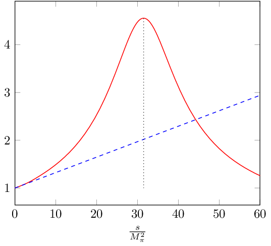
We next turn toward the partial-wave projection $f_{1}^{K^{+}\pi^{-}\to\pi^{+}\pi^{-}}(s)$ , to which we wish to apply the same procedure. Starting from its one-loop expression obtained in App. B, and neglecting the contributions from the circular cuts, the IAM-unitarized version of $f_{1}^{K^{+}\pi^{-}\to\pi^{+}\pi^{-}}(s)$ reads [ $\psi_{+}^{\rm loop}(s)$ is defined in eq. (B.19)]

f_{1}^{K^{+}\pi^{-}\to\pi^{+}\pi^{-}}(s)\\ =\frac{\left[{\displaystyle{\frac{\alpha_{+}}{96\pi M_{\pi}^{2}}}}\right]^{2}\times\lambda_{K\pi}^{1/2}(s)\sqrt{1-\frac{4M_{\pi}^{2}}{s}}}{{\displaystyle{\frac{1}{96\pi M_{\pi}^{2}}}}\bigg[\alpha_{+}-\beta_{+}\frac{s-s_{0}}{M_{\pi}^{2}}\bigg]-\psi_{+}^{\rm loop}(s)+{\rm Re}\,\psi_{+}^{\rm loop}(s_{0})+(s-s_{0}){\rm Re}\,\psi_{+}^{\rm loop~\prime}(s_{0})}.

(6.9)

We will further simplify this expression upon keeping only the contribution of the unitarity or right-hand cut of $\psi_{+}^{\rm loop}(s)$ into account, i.e. the first term on the right-hand side of eq. (B.19). The remaining terms give only a small correction in comparison. We thus end up with

f_{1}^{K^{+}\pi^{-}\to\pi^{+}\pi^{-}}(s)\\ =\frac{{\displaystyle{\frac{\alpha_{+}}{96\pi M_{\pi}^{2}}}}\times\lambda_{K\pi}^{1/2}(s)\sqrt{1-\frac{4M_{\pi}^{2}}{s}}}{1-{\displaystyle{\frac{\beta_{+}}{\alpha_{+}}\frac{s-s_{0}}{M_{\pi}^{2}}}}-{\displaystyle{\frac{\beta}{6}\frac{s-4M_{\pi}^{2}}{F_{\pi}^{2}}}}\left[{\bar{J}}_{\pi\pi}(s)-{\rm Re}\,{\bar{J}}_{\pi\pi}(s_{0})\right]+{\displaystyle{\frac{\beta}{6}\frac{s_{0}-4M_{\pi}^{2}}{F_{\pi}^{2}}}}(s-s_{0}){\rm Re}\,{\bar{J}}_{\pi\pi}^{\prime}(s_{0})}.~~~

(6.10)

If we transpose the discussion that follows eq. (6.8) to the representation (6.10), we observe that, when the contributions from the pion loops are discarded, the “bare” pole is located at a value of $s$ given by $s_{\rm pole}=s_{0}+(\alpha_{+}/\beta_{+})M_{\pi}^{2}$ . For the values given in eq. (3.17), i.e. $\alpha_{+}/\beta_{+}\sim 7$ , this gives $s_{\rm pole}\sim 12M_{\pi}^{2}$ . In order to obtain a pole located at $s_{\rm pole}\sim M_{\rho}^{2}$ , one needs a higher value of the ratio $\alpha_{+}/\beta_{+}$ , say $\alpha_{+}/\beta_{+}\sim 25$ . In view of the error bars of the numerical values of $\alpha_{+}$ and $\beta_{+}$ , this can be achieved most economically upon increasing $\beta_{+}$ by about two standard deviations from its central value in eq. (3.17). Assigning even part of the effect to an increase of the absolute value of $\alpha_{+}$ would represent a much more significant deviation from its value in (3.17). At this stage one might recall the discussion in Sec. 4, where it was already noticed that upon keeping $\beta_{+}$ as a free variable to be fitted to the data, the outcome was favouring values deviating from the one in (3.17) by a similar amount. It would certainly appear as somewhat far-fetched to ground the reason for preferring larger values of $\beta_{+}$ on the simple characteristics of the IAM-unitarized partial wave $f_{1}^{K^{+}\pi^{-}\to\pi^{+}\pi^{-}}(s)$ . Nevertheless, the concordance, on this issue, with the analysis presented in Sec. 4 is definitely interesting and noteworthy²² 2 For the sake of completeness, let us mention that the Dalitz plot of the $K^{+}\rightarrow\pi^{+}\pi^{+}\pi^{-}$ transition has been measured with high precision by the NA-48/2 Collaboration Batley:2007md. These results were published after ref. Bijnens:2002vr. Using only ref. Batley:2007md does not allow for a separate determination of $\alpha_{+}$ and $\beta_{+}$ but only of the ratio $\alpha_{+}/\beta_{+}$ . In terms of the Dalitz plot parameters $g,h$ and $k$ of ref. Batley:2007md, one obtains $\alpha_{+}/\beta_{+}\sim-g/(h-3k)=6.53(1)$ in agreement with the value obtained from eq. (3.17).. In figure 9, we illustrate the evolution of $|f_{1}^{K^{+}\pi^{-}\to\pi^{+}\pi^{-}}(s)|$ as given in eq. (6.10) for different values of $\beta_{+}$ and for $s\geq 4M_{\pi}^{2}$ . Notice also that the approximation considered in eq. (6.10) preserves Watson’s final-state theorem, and the phases of $F_{V}^{\pi}(s)$ and of $f_{1}^{K^{+}\pi^{-}\to\pi^{+}\pi^{-}}(s)$ should be identical. For the choice $\beta=1.11$ [this value of $\beta$ is itself chosen such as to match the phase of the pion form factor to the phase of the $P$ -wave projection of the $\pi\pi$ amplitude, both obtained upon unitarization of their one-loop expressions by the IAM method], this is the case for $\beta_{+}=-0.85\cdot 10^{-8}$ .

The numerical evaluation of the two sum rules in eq. (6.7) for these values of $\beta$ and of $\beta_{+}$ then gives

a_{+}^{\pi\pi}=-1.58,\quad b_{+}^{\pi\pi}=-0.76.

(6.11)

In this approach, the overall negative sign of these numbers is driven by the negative sign of $\alpha_{+}$ . The result for $b_{+}$ comes out relatively close to the values extracted from the data in Sec. 4, whereas the absolute value of $a_{+}$ is about twice as large. Of course, in both cases there are other contributions which we need to discuss before being in a position of making a more definite statement.

Let us finally notice that the same approach can also be implemented in order to evaluate the contribution from the two-pion state to $a_{S}$ and $b_{S}$ . It suffices to make the appropriate replacements in eq. (6.10). We first notice that a ratio $\alpha_{S}/\beta_{S}\sim 25$ lies (almost) within reach for the values indicated in eq. (3.18), e.g. $\alpha_{S}\sim-7.5\cdot 10^{-8}$ , $\beta_{S}\sim-0.3\cdot 10^{-8}$ . The resulting values of $a_{S}^{\pi\pi}$ and $b_{S}^{\pi\pi}$ would then also be negative, and about three times smaller in absolute value than those obtained for $a_{+}^{\pi\pi}$ and $b_{+}^{\pi\pi}$ in eq. (6.11).

6.2 Intermediate states with higher thresholds

In Sec. 2.2, we have established the high-energy behaviour of the dimensionally renormalized form factor, see eq. (2.29). Reproducing this behaviour is necessary in order to obtain an amplitude that does no longer depend on the short-distance renormalization scale $\nu$ once the contribution from the local factorized operator $Q_{7V}$ is added. This behaviour is, however, not reproduced by the contribution of the $\pi\pi$ intermediate state that we have just studied. It has therefore to come from the remaining infinite number of intermediate states, with higher and higher thresholds, and which eventually end up into the perturbative contribution of quarks and gluons at short distances. One might attempt to describe some of these additional intermediate states in a similar treatment as the one adopted here for the two-pion states. This holds, in particular, for the next thresholds, due to $K\pi$ and to ${\bar{K}}K$ intermediate states. We leave such improvements for future work. Here, we will adopt a simpler point of view, where the additional intermediate states are described by zero-width resonance states. Such a picture would naturally emerge, for instance, from the perspective of the limit where the number of colours $N_{c}$ becomes large tHooft74; Witten79. Contributions of this type are depicted on figure 10, and would produce a form factor with the following expression

W_{+}^{\rm res}(z;\nu)=\sum_{V=\phi\cdots}\frac{f_{V}{\widetilde{g}}_{V}}{s-M_{V}^{2}+i0}\,+\sum_{V=K^{*}\cdots}\frac{g_{V}{\widetilde{f}}_{V}}{s-M_{V}^{2}+i0}.

(6.12)

The first sum runs over resonances with quantum numbers $J^{PC}=1^{--}$ , $I=1$ , $S=0$ . It starts here with the $\phi(1020)$ , since the $\rho$ meson is already contained in the contribution of the $\pi\pi$ intermediate states that we have discussed previously. The second sum runs over the resonances with quantum numbers $J^{P}=1^{-}$ , $I=1/2$ , $S=\pm 1$ , and starts with the $K^{*}(892)$ . The strong couplings $f_{V}$ and $g_{V}$ are fixed, for instance, by the widths of the decays like $\phi\to e^{+}e^{-}$ and $K^{*}\to K\pi$ , respectively. Information on the weak couplings ${\widetilde{f}}_{V}$ and ${\widetilde{g}}_{V}$ is, however, not available. This represents the usual difficulty in obtaining reliable estimates of the low-energy constants in the weak sector through resonance saturation Ecker:1992de; Ecker:1990in; Pich:1990mw; DAmbrosio:1997ctq; Cappiello:2011re. Another difficulty lies in the fact that the correct short-distance behaviour (2.29) can only be recovered upon considering an infinite number of resonances Witten79. This second difficulty can be dealt with upon using available techniques Greynat:2013cta; Shifman:2000jv; Rafael:2012sy to construct resonance models with spectra of the Regge-type, and with residues that can be tuned such as to build up harmonic sums that can often be resummed exactly and, moreover, reproduce the prescribed asymptotic behaviour. We will present such a construction in the case of interest here.

In order to set the stage, let us go back to the calculation in Section 2.2. It teaches us that a dispersive representation of the type

W_{+}(z)=\frac{f^{K^{\pm}\pi^{\mp}}_{+}(zM_{K}^{2})}{4\pi}\int dx\frac{\rho_{M}(x)}{x-zM_{K}^{2}-i0},\quad\rho_{M}(s)=A\theta(s-M^{2})\,\sqrt{1-\frac{M^{2}}{s}},

(6.13)

would fulfill the required conditions. Here $A$ is a normalization constant, and $M$ is a mass scale which corresponds to the onset of the perturbative continuum due to the quark loop, and which we would like to identify with a typical resonance scale $M\sim 1$ GeV. Of course, the above dispersive integral does not converge, and we first need to consider the dimensionally regularized version of the spectral density $\rho_{M}(s)$ , namely Gasser:1998qt

\rho_{M}(s;D)=A(D)(4\pi)^{2-\frac{D}{2}}\left(\frac{M^{2}}{\nu_{\mbox{\tiny MS}}^{2}}\right)^{\frac{D}{2}-2}\frac{\Gamma\left(\frac{3}{2}\right)}{\Gamma\left(\frac{D}{2}-\frac{1}{2}\right)}\left(\frac{s}{M^{2}}-1\right)^{\frac{D}{2}-2}\,\sqrt{1-\frac{M^{2}}{s}}\,\theta(s-M^{2}),

(6.14)

where the function $A(D)$ is only constrained by the condition $A(4)=A$ , $A(D)=A+(D-4)A^{\prime}+\cdots$ , and $A^{\prime}$ parameterizes the scheme-dependence arising from the Dirac matrices in the calculation of Section 2.2. The divergence of the dispersive integral is then contained in the value of the integral at $z=0$ ,

$\displaystyle\int\!dx\,\frac{\rho_{M}(x;D)}{x}$	$\displaystyle=$	$\displaystyle A(D)(4\pi)^{2-\frac{D}{2}}\!\left(\frac{M^{2}}{\nu_{\mbox{\tiny MS}}^{2}}\right)^{\frac{D}{2}-2}\!\!\frac{\Gamma\!\left(\frac{3}{2}\right)}{\Gamma\!\left(\frac{D}{2}-\frac{1}{2}\right)}\frac{\Gamma\!\left(\frac{D}{2}-\frac{1}{2}\right)\Gamma\!\left(2-\frac{D}{2}\right)}{\Gamma\!\left(\frac{3}{2}\right)}$	(6.15)
	$\displaystyle=$	$\displaystyle A(D)(4\pi)^{2-\frac{D}{2}}\left(\frac{M^{2}}{\nu_{\mbox{\tiny MS}}^{2}}\right)^{\frac{D}{2}-2}\!\Gamma\!\left(2-\frac{D}{2}\right)$
	$\displaystyle=$	$\displaystyle A\left[\frac{-2}{D-4}-\gamma_{E}+\ln(4\pi)-\ln\frac{M^{2}}{\nu_{\mbox{\tiny MS}}^{2}}-2A^{\prime}/A+\cdots\right].$

After renormalization in the ${\overline{\rm MS}}$ scheme, one therefore finds

W_{+}(z;\nu)=f^{K^{\pm}\pi^{\mp}}_{+}(zM_{K}^{2})\\ \times\frac{1}{4\pi}\bigg[zM_{K}^{2}\int\frac{dx}{x}\,\theta(x-M^{2})\,\sqrt{1-\frac{M^{2}}{x}}\frac{A}{x-zM_{K}^{2}-i0}-A\ln\frac{M^{2}}{\nu^{2}}-2A^{\prime}\bigg].

(6.16)

The limit of large space-like values of $z$ gives

\lim_{z\to-\infty}W_{+}(z;\nu)/f^{K^{\pm}\pi^{\mp}}_{+}(zM_{K}^{2})=\frac{1}{4\pi}\bigg[2(A-A^{\prime}-A\ln 2)-A\ln\frac{-zM_{K}^{2}}{\nu^{2}}\bigg].

(6.17)

The short-distance behaviour given in eq. (2.29) is then recovered in this case with the choices

	$\displaystyle A$	$\displaystyle=16\pi^{2}M_{K}^{2}\left(\frac{G_{\rm F}}{\sqrt{2}}V_{us}^{*}V_{ud}\right)\sum_{I}C_{I}(\nu)\xi_{01}^{I},$
	$\displaystyle A^{\prime}$	$\displaystyle=-16\pi^{2}M_{K}^{2}\left(\frac{G_{\rm F}}{\sqrt{2}}V_{us}^{*}V_{ud}\right)\sum_{I}C_{I}(\nu)\left[\frac{1}{2}\xi_{00}^{I}-(1-\ln 2)\xi_{01}^{I}\right].$		(6.18)

Actually, the dispersive integral (6.13) with $\rho_{M}(x;D)$ can be done explicitly $(w\equiv-zM_{K}^{2}/M^{2})$ :

\int dx\,\frac{\rho_{M}(x;D)}{x-zM_{K}^{2}}=A(D)(4\pi)^{2-\frac{D}{2}}\left(\frac{M^{2}}{\nu_{\mbox{\tiny MS}}^{2}}\right)^{\frac{D}{2}-2}\,\Gamma\left(2-\frac{D}{2}\right)\times{}_{2}\mathrm{F}_{1}\left(\begin{tabular}[]{c}$1$ , $2-\frac{D}{2}$\\ $\frac{3}{2}$\end{tabular}\Bigg|-w\right).

(6.19)

For the definition and properties of the hypergeometric function ${{}_{2}}\mathrm{F}_{1}$ , we refer the reader to ref. DLMF. The properties (6.15) and (6.17) can then be directly recovered from those of this function, see e.g. (DLMF, eq. 15.8.2),

\hskip-14.22636pt{{}_{2}}\mathrm{F}_{1}\!\left(\left.\begin{matrix}1\,,\,2-\frac{D}{2}\\ \frac{3}{2}\end{matrix}\right|-w\right)=\left\{\begin{tabular}[]{l}$1+\mathcal{O}(w)$~~~[$w\rightarrow 0$]\\ \\ $\frac{\pi^{\frac{3}{2}}}{2\sin\left(\pi\frac{4-D}{2}\right)}\frac{1}{\Gamma\left(\frac{4-D}{2}\right)\Gamma\left(\frac{D-1}{2}\right)}\;w^{-\frac{4-D}{2}}\left[1+\mathcal{O}(w^{-1})\right]$ ~~~[$w\rightarrow+\infty$]\end{tabular}\right..

(6.20)

It is possible to reproduce the salient properties of the simple model discussed above through a Regge-type resonance model of the form

	$\displaystyle\rho^{K\pi}_{\rm res}(s;D)$	$\displaystyle=$	$\displaystyle A(D)(4\pi)^{2-\frac{D}{2}}\left(\frac{M^{2}}{\nu_{\mbox{\tiny MS}}^{2}}\right)^{\frac{D}{2}-2}\,\Gamma\left(2-\frac{D}{2}\right)\sum_{n\geq 1}M^{2}\mu_{n}(D)\delta(s-nM^{2}),$
	$\displaystyle\int dx\,\frac{\rho^{K\pi}_{\rm res}(x;D)}{x+wM^{2}}$	$\displaystyle=$	$\displaystyle A(D)(4\pi)^{2-\frac{d}{2}}\left(\frac{M^{2}}{\nu_{\mbox{\tiny MS}}^{2}}\right)^{\frac{D}{2}-2}\,\Gamma\left(2-\frac{D}{2}\right)\sum_{n\geq 1}\frac{\mu_{n}(D)}{(n+w)},$

provided one can find a set of functions $\mu_{n}(D)$ that satisfies the following requirements:

•

$\sum_{n\geq 1}\frac{\mu_{n}(D)}{n}=1$
•

$\mu_{n}(D)\underset{D\rightarrow 4}{=}(D-4){\bar{\mu}}_{n}+{\cal O}\left((D-4)^{2}\right)$
•

$\xi(w)\equiv\sum_{n\geq 1}\frac{{\bar{\mu}}_{n}}{n(n+w)}$ converges
•

$\xi(w)\underset{w\rightarrow+\infty}{\sim}\ln w$

As we now show, a solution, by far not unique, to this list of requirements can then be constructed in the form

\mu_{n}(D)=\mathsf{a}(D)\,n^{\frac{D-4}{2}}+\mathsf{b}(D)\,n^{2}\left(\frac{D}{2}-1\right)^{n},

(6.22)

for suitably chosen functions $\mathsf{a}(D)$ and $\mathsf{b}(D)$ . Indeed, starting from the inverse Mellin representation

\frac{1}{1+\frac{w}{n}}=\int\limits_{c_{1}-i\infty}^{c_{1}+i\infty}\!\frac{du}{2i\pi}\left(\frac{w}{n}\right)^{-u}\;\frac{\pi}{\sin\pi u}\;,

(6.23)

valid for $0<c_{1}<1$ , and making use of the sums

\sum_{n=1}^{\infty}n^{\frac{D-4}{2}+u-1}=\zeta\!\left(\frac{6-D}{2}-u\right),\qquad\sum_{n=1}^{\infty}\left(\frac{D}{2}-1\right)^{n}n^{u+1}={\rm Li}_{-1-u}\left(\frac{D}{2}-1\right),

(6.24)

one obtains

\sum_{n=1}^{\infty}\left[\mathsf{a}\,n^{\frac{D-4}{2}}+\mathsf{b}\,n^{2}\left(\frac{D}{2}-1\right)^{n}\right]\frac{1}{n+w}\\ =\int\limits_{c_{2}-i\infty}^{c_{2}+i\infty}\!\frac{du}{2i\pi}\;w^{-u}\;\frac{\pi}{\sin\pi u}\left[\mathsf{a}\,\zeta\!\left(\frac{6-D}{2}-u\right)+\mathsf{b}\,{\rm Li}_{-1-u}\left(\frac{D}{2}-1\right)\right]\;,

(6.25)

with $0<c_{2}<\frac{4-D}{2}$ . Here $\zeta(x)$ is the Riemann $\zeta$ -function and ${\rm Li}_{y}(x)$ denotes the polylogarithm function, defined as ${\rm Li}_{y}(x)=\sum_{n>0}x^{n}n^{-y}$ for $|x|<1$ and arbitrary complex $y$ , and by analytic continuation for other values of $x$ . The integrand in the relation (6.25) has a pole at $u=0$ , coming from the pre-factor only, since the terms inside the square brackets are well behaved at $u=0$ , with ${\rm Li}_{-1}(x)=x/(1-x)^{2}$ . According to the Converse Mapping Theorem FGD95; Friot:2005cu, from this pole at $u=0$ , located on the left of the fundamental strip $0<c_{2}<\frac{4-D}{2}$ , one deduces that

\sum_{n=1}^{\infty}\left[\mathsf{a}\,n^{\frac{D-4}{2}}+\mathsf{b}\,n^{2}\left(\frac{D}{2}-1\right)^{n}\right]\frac{1}{n+w}\underset{w\rightarrow 0}{\sim}\mathsf{a}\,\zeta\!\left(\frac{6-D}{2}\right)+2\mathsf{b}\,\frac{D-2}{(D-4)^{2}}.

(6.26)

Since $\zeta(3-D/2-u)\to-1/(u-2+D/2)+\cdots$ for $u\to 2-D/2$ , while ${\rm Li}_{-1-u}(D/2-1)$ remains finite as this limit is taken, the integrand has also a pole at $u=\frac{4-D}{2}$ , due to the first term in the square brackets. In this case, the pole being located on the right of the fundamental strip $0<c_{2}<\frac{4-D}{2}$ , the Converse Mapping Theorem allows us to state that

\sum_{n=1}^{\infty}\left[\mathsf{a}\,n^{\frac{D-4}{2}}+\mathsf{b}\,n^{2}\left(\frac{D}{2}-1\right)^{n}\right]\frac{1}{n+w}\underset{w\rightarrow\infty}{\sim}\mathsf{a}\,\frac{\pi}{\sin\left(\pi\frac{4-D}{2}\right)}\;w^{-\frac{4-D}{2}}.

(6.27)

We thus conclude that we are able to build a Regge-type resonance model, defined by eq. (6.22), with

\mathsf{a}(D)=\frac{\frac{\sqrt{\pi}}{2}}{\Gamma\left(\frac{4-D}{2}\right)\Gamma\left(\frac{D-1}{2}\right)}\;\;\text{and}\;\;\mathsf{b}(D)=\frac{1}{2}\,\frac{(D-4)^{2}}{D-2}\left[1-\frac{\frac{\sqrt{\pi}}{2}\zeta\!\left(\frac{6-D}{2}\right)}{\Gamma\left(\frac{4-D}{2}\right)\Gamma\left(\frac{D-1}{2}\right)}\right],

(6.28)

and which satisfies all the required properties. The part of the integral that remains finite in the limit $D\to 4$ can be resummed explicitly, and we find

\int dx\,\frac{\rho_{\rm res}(x;D)}{x-zM_{K}^{2}}\\ =A(D)(4\pi)^{\frac{4-D}{2}}\left(\frac{M^{2}}{\nu^{2}_{\text{MS}}}\right)^{\frac{D-4}{2}}\,\Gamma\left(\frac{4-D}{2}\right)-A\left[\gamma_{E}+\psi(1+w)\right]+{\cal O}(D-4),

(6.29)

where the di-gamma function $\psi$ arises through the sum

\sum_{n=1}^{\infty}\frac{w}{n(n+w)}=\gamma_{E}+\psi(1+w).

(6.30)

Actually, considering more generally the poles when $u$ equals a negative integer, the Converse Mapping Theorem gives

\sum_{n=1}^{\infty}\left[\mathsf{a}(D)\,n^{\frac{D-4}{2}}+\mathsf{b}(D)\,n^{2}\left(\frac{D}{2}-1\right)^{n}\right]\frac{1}{n+w}\ \underset{w\rightarrow 0}{\sim}\ \sum_{p=0}^{N}(-1)^{p}\mathsf{c}_{p}(D)w^{p}+{\mathcal{O}}(w^{N+1}),

(6.31)

with the coefficients $\mathsf{c}_{p}(D)$ given by $\mathsf{c}_{0}(D)=1$ and, for $p>0$ , by

\mathsf{c}_{p}(D)=\mathsf{a}(D)\,\zeta\!\left(\frac{6+2p-D}{2}\right)+\mathsf{b}(D)\,{\rm Li}_{p-1}\left(\frac{D}{2}-1\right)\qquad[p\geq 1].

(6.32)

In the limit where $D\to 4$ , one obtains

\Gamma\left(\frac{4-D}{2}\right)\mathsf{c}_{p}(D)\to\zeta(p+1),

(6.33)

which indeed corresponds to eq. (6.29).

Summarizing, we end up, after minimal subtraction, with the expression

W_{+}^{\rm res}(z;\nu)=\frac{f^{K^{\pm}\pi^{\mp}}_{+}(zM_{K}^{2})}{4\pi}\\ \times 16\pi^{2}M_{K}^{2}\left(\frac{G_{\rm F}}{\sqrt{2}}V_{us}^{*}V_{ud}\right)\sum_{I}C_{I}(\nu)\bigg\{\xi_{00}^{I}-\xi_{01}^{I}\left[\ln\frac{M^{2}}{\nu^{2}}+\psi\left(1-z\,\frac{M_{K}^{2}}{M^{2}}\right)\right]\bigg\}.

(6.34)

Accordingly, the corresponding contributions to $a_{+}$ and $b_{+}$ read [cf. eq. (3.19)],

G_{F}M_{K}^{2}a_{+}^{\rm res}(\nu)=W_{+}^{\rm res}(0;\nu),\quad G_{F}M_{K}^{2}b_{+}^{\rm res}(\nu)=W_{+}^{{\rm res}\,\prime}(0;\nu),

(6.35)

i.e.

$\displaystyle a_{+}^{\rm res}(\nu)$	$\displaystyle=$	$\displaystyle\frac{f^{K^{\pm}\pi^{\mp}}_{+}(0)}{4\pi}\times 16\pi^{2}\left(\frac{1}{\sqrt{2}}V_{us}^{*}V_{ud}\right)\sum_{I}C_{I}(\nu)\bigg\{\xi_{00}^{I}-\xi_{01}^{I}\left[\ln\frac{M^{2}}{\nu^{2}}-\gamma_{E}\right]\bigg\},$
$\displaystyle b_{+}^{\rm res}(\nu)$	$\displaystyle=$	$\displaystyle\frac{f^{K^{\pm}\pi^{\mp}}_{+}(0)}{4\pi}\times 16\pi^{2}\left(\frac{1}{\sqrt{2}}V_{us}^{*}V_{ud}\right)\,\frac{\pi^{2}}{6}\,\frac{M_{K}^{2}}{M^{2}}\sum_{I}C_{I}(\nu)\,\xi_{01}^{I}$	(6.36)
		$\displaystyle\!\!\!\!\!+\,\frac{f^{K^{\pm}\pi^{\mp}}_{+}(0)}{4\pi}\times\lambda_{+}\,\frac{M_{K}^{2}}{M_{\pi}^{2}}$
		$\displaystyle\hskip 56.9055pt\times 16\pi^{2}\left(\frac{1}{\sqrt{2}}V_{us}^{*}V_{ud}\right)\sum_{I}C_{I}(\nu)\bigg\{\xi_{00}^{I}-\xi_{01}^{I}\left[\ln\frac{M^{2}}{\nu^{2}}-\gamma_{E}\right]\bigg\}.$

The expression of $b_{+}^{\rm res}(\nu)$ involves the slope at the origin $\lambda_{+}$ of the form factor $f^{K^{\pm}\pi^{\mp}}_{+}(s)$ . It is defined in eq. (A.1), and numerical values for both $f^{K^{\pm}\pi^{\mp}}_{+}(0)$ and $\lambda_{+}$ are given in eq. (A.3).

We draw attention here to the fact that only the order $\mathcal{O}(\alpha_{s}^{0})$ contribution to the short distance behaviour of $W(s;\nu)$ is reproduced by the resonance model. This means that eq. (6.34) satisfies both (2.15) and (2.29) at order $\mathcal{O}(\alpha_{s}^{0})$ only, which implies that some scale dependence will remain. We could improve on this aspect upon including $\mathcal{O}(\alpha_{s})$ corrections, which are almost completely determined from the renormalization-group analysis in Sec. 2.2. We would then need to build a resonance model that reproduces both the correct $\ln(-s/\nu^{2})$ and $\ln^{2}(-s/\nu^{2})$ behaviours at high energy. We leave such an improvement for a future study.

6.3 The contribution from the factorized $\boldsymbol{Q_{7V}}$ operator

It remains to evaluate the last contribution, due to $W_{+}^{\rm SD}(z;\nu)$ . From its definition in eq. (6.6), combined with eq. (3.19), we obtain right away

	$\displaystyle a_{+}^{\rm SD}(\nu)$	$\displaystyle=\frac{f^{K^{\pm}\pi^{\mp}}_{+}(0)}{4\pi}\times 16\pi^{2}\left(\frac{1}{\sqrt{2}}V_{us}^{*}V_{ud}\right)\frac{C_{7V}(\nu)}{\alpha}$
	$\displaystyle b_{+}^{\rm SD}(\nu)$	$\displaystyle=\frac{f^{K^{\pm}\pi^{\mp}}_{+}(0)}{4\pi}\times\lambda_{+}\,\frac{M_{K}^{2}}{M_{\pi}^{2}}\times 16\pi^{2}\left(\frac{1}{\sqrt{2}}V_{us}^{*}V_{ud}\right)\frac{C_{7V}(\nu)}{\alpha}.$		(6.37)

Values for $C_{7V}$ can be found in ref. Buras:1994qa. In particular, we use $C_{7V}^{({\rm NDR,HV})}(1~{\rm GeV})/\alpha=(-0.037,0.000)$ . Here we have set $\tau=0$ , i.e. we have identified $C_{7V}$ with $z_{7V}$ , and we have chosen $\Lambda^{(4)}_{\overline{\rm MS}}=300~{\rm MeV}$ . In order to investigate the dependence of the sums $a_{+}^{\rm res}(\nu)+a_{+}^{\rm SD}(\nu)$ and $b_{+}^{\rm res}+b_{+}^{\rm SD}(\nu)$ on the short-distance scale $\nu$ , we use the lowest-order evolution equations, neglecting the mixing with the penguin operators, i.e.

\frac{C_{7V}(\nu)}{\alpha}=\frac{C_{7V}(\nu_{0})}{\alpha}+\frac{16}{99}\left[1-\left(\frac{\alpha_{s}^{(3)}(\nu)}{\alpha_{s}^{(3)}(\nu_{0})}\right)^{-11/9}\right]\frac{C_{+}(\nu_{0})}{\alpha_{s}(\nu_{0})}-\frac{8}{45}\left[1-\left(\frac{\alpha_{s}^{(3)}(\nu)}{\alpha_{s}^{(3)}(\nu_{0})}\right)^{-5/9}\right]\frac{C_{-}(\nu_{0})}{\alpha_{s}(\nu_{0})},

(6.38)

where $C_{\pm}(\nu)=C_{2}(\nu)\pm C_{1}(\nu)$ and

C_{+}(\nu)=\left(\frac{\alpha_{s}^{(3)}(\nu)}{\alpha_{s}^{(3)}(\nu_{0})}\right)^{-2/9}C_{+}(\nu_{0})\;,\;\;C_{-}(\nu)=\left(\frac{\alpha_{s}^{(3)}(\nu)}{\alpha_{s}^{(3)}(\nu_{0})}\right)^{4/9}C_{-}(\nu_{0}).

(6.39)

Here $\alpha_{s}^{(3)}$ stands for the running QCD coupling for $N_{f}=3$ active flavours,

\alpha_{s}^{(N_{f})}(\nu)=\frac{12\pi}{(33-2N_{f})t^{(N_{f})}(\nu)},\quad t^{(N_{f})}(\nu)\equiv 2\ln(\nu/\Lambda^{(N_{f})}_{\overline{\rm MS}}),

(6.40)

and for the numerical evaluation, we use $\Lambda^{(3)}_{\overline{\rm MS}}=340~{\rm MeV}$ and the following input values Buras:1994qa

C_{+}(1~{\rm GeV})=\left\{\begin{tabular}[]{ll}0.771&NDR\\ 0.735&HV\end{tabular}\right.,\quad C_{-}(1~{\rm GeV})=\left\{\begin{tabular}[]{ll}1.737&NDR\\ 1.937&HV\end{tabular}\right.

(6.41)

6.4 Evaluations of $\boldsymbol{a_{+}}$ and $\boldsymbol{b_{+}}$

Collecting the various contributions to $a_{+}$ and to $b_{+}$ from the model proposed in this section, we end up, according to eq. (3.19), with the following expressions :

$\displaystyle a_{+}$	$\displaystyle=$	$\displaystyle\int_{0}^{\infty}\frac{dx}{x}\,\frac{\rho_{+}^{\pi\pi}(x)}{G_{F}M_{K}^{2}}$
		$\displaystyle\hskip 28.45274pt+\frac{f^{K^{\pm}\pi^{\mp}}_{+}(0)}{4\pi}\times 16\pi^{2}\left(\frac{1}{\sqrt{2}}V_{us}^{*}V_{ud}\right)\bigg\{\frac{C_{7V}(\nu)}{\alpha}+\sum_{I}C_{I}(\nu)\bigg[\xi_{00}^{I}-\xi_{01}^{I}\left(\ln\frac{M^{2}}{\nu^{2}}-\gamma_{E}\right)\bigg]\bigg\},$
$\displaystyle b_{+}$	$\displaystyle=$	$\displaystyle\int_{0}^{\infty}\frac{dx}{x^{2}}\,\frac{\rho_{+}^{\pi\pi}(x)}{G_{F}}+\frac{f^{K^{\pm}\pi^{\mp}}_{+}(0)}{4\pi}\times 16\pi^{2}\left(\frac{1}{\sqrt{2}}V_{us}^{*}V_{ud}\right)\,\frac{\pi^{2}}{6}\,\frac{M_{K}^{2}}{M^{2}}\sum_{I}C_{I}(\nu)\,\xi_{01}^{I}$	(6.42)
		$\displaystyle+\,\frac{f^{K^{\pm}\pi^{\mp}}_{+}(0)}{4\pi}\times\lambda_{+}\,\frac{M_{K}^{2}}{M_{\pi}^{2}}\times 16\pi^{2}\left(\frac{1}{\sqrt{2}}V_{us}^{*}V_{ud}\right)\bigg\{\frac{C_{7V}(\nu)}{\alpha}+\sum_{I}C_{I}(\nu)\bigg[\xi_{00}^{I}-\xi_{01}^{I}\left(\ln\frac{M^{2}}{\nu^{2}}-\gamma_{E}\right)\bigg]\bigg\}$
		$\displaystyle-\,\frac{1}{60}\,\left(\frac{M_{K}^{2}}{M_{\pi}^{2}}\right)^{2}{\alpha_{+}\left(1-\frac{\beta_{+}}{\alpha_{+}}\frac{s_{0}}{M_{\pi}^{2}}\right)}.$

Numerically, for $1\,{\rm GeV}\leqslant\nu\leqslant 2\,{\rm GeV}$ , $M=1\,{\rm GeV}$ , and considering only contributions from $C_{1}$ and $C_{2}$ , one obtains

\displaystyle a_{+}=-1.58+\begin{cases}[-0.10,0.03]&{\rm NDR}\\ [-0.14,0.07]&{\rm HV}\end{cases}

\displaystyle b_{+}=-0.76+\begin{cases}[-0.04,0.03]&{\rm NDR}\\ [-0.07,0.03]&{\rm HV}\end{cases}.

(6.43)

The residual $\nu$ -dependence of $a_{+}$ and $b_{+}$ is depicted in figure 11.

This result should mainly be viewed as a first serious attemp to evaluate $a_{+}$ and $b_{+}$ . Improvements, for instance on the description of $W_{+}^{\pi\pi}(z)$ , or the inclusion of QCD corrections in $W_{+}^{\rm res}(z)$ , are clearly required before realistic error bars can be assigned to the values displayed in eq. (6.42). We come back to these issues in the next section. Nevertheless, we find it encouraging that the outcome of the rather simple approach followed in the present section comes rather close to the values obtained from the experimental data in Sec. 4. This is particularly true for $b_{+}$ .

7 Summary, conclusions, outlook

In this final section, we wish to summarize the content of this article, going successively through the main aspects of the issues that have been addressed, roughly following the list of items given at the end of the introduction. For each item, we provide conclusions and/or critical remarks, as well as an outline of perspectives for future improvements.

7.1 Extracting $\boldsymbol{a_{+,S}}$ and $\boldsymbol{b_{+,S}}$ from recent data

Our first concern was to establish the values of the constants $a_{+,S}$ and $b_{+,S}$ that are provided by recent experimental data. In the case of $K^{\pm}\to\pi^{\pm}e^{+}e^{-}$ , we have shown that a combined fit to the data on the decay distribution from the two high-statistics experiments BNL-E865 and NA48/2 clearly favours the solution where $a_{+}$ and $b_{+}$ are both negative, with $|a_{+}|$ and $|b_{+}|$ comparable in size.

We have also performed fits to the data keeping, in addition to $a_{+}$ and $b_{+}$ , the curvature $\beta_{+}$ of the $K^{\pm}\to\pi^{\pm}\pi^{+}\pi^{-}$ Dalitz plot as a free parameter, and have found that somewhat smaller (in absolute value) values than those obtained by direct determinations from $K\to\pi\pi\pi$ data are preferred.

In order to make comparisons between different approaches more convenient, we have introduced intrinsic definitions of the coefficients $a_{+,S}$ and $b_{+,S}$ in terms of the values of the form factors and of their slopes at the origin $z=0$ .

7.2 The low-energy expansion of the form factors to two loops

The extraction of $a_{+,S}$ and $b_{+,S}$ from data was done using the expressions $W_{+,S;{\rm b1L}}(z)$ of the form factors given in ref. DAmbrosio:1998gur. Our second concern was then to establish whether two-loop corrections not accounted for by these expressions might have an effect on these determinations.

We have provided the full two-loop expression of the form factors, taking only the singularities due to two-pion intermediate states into account, in analogy with ref. DAmbrosio:1998gur. These two-loop expressions are based on the complete one-loop expression of the partial-wave projections $f_{1}^{K\pi\to\pi^{+}\pi^{-}}(s)$ , which include also $\pi\pi$ rescattering in the crossed channels. These features are not accounted for by the expressions of $W_{+,S;{\rm b1L}}(z)$ given in ref. DAmbrosio:1998gur.

From a numerical point of view, these effects turn out to be quite small in the region of $z$ corresponding to the phase space for the the $K\to\pi\ell^{+}\ell^{-}$ decays. In practice, one may thus use the simpler form $W_{\rm b1L}(z)$ in order to analyze the data, instead of the full two-loop expression $W_{\rm 2L}(z)$ , without significant impact on the determinations of $a_{+,S}$ and $b_{+,S}$ . This also strongly suggests that still higher-order corrections are quite small and are likely not to modify the picture in any substantial way.

We have also pointed out that the existing one-loop calculations suggest that kaon loops could possibly have a sizeable effect on $a_{+}$ and $a_{S}$ . However, making a quantitative statement on this issue would require a complete two-loop calculation in the usual framework of three-flavour chiral perturbation theory, including the computation of those Feynman graphs that do not exhibit non-trivial analyticity properties.

7.3 Contribution from the two-pion state

We have addressed the phenomenological evaluation of the contribution from the two-pion state to $a_{+}$ and $b_{+}$ upon writing an unsubtracted dispersion relation for the form factor $W_{+}(z)$ , from which sum rules for $a_{+}$ and $b_{+}$ can be obtained. The absorptive part of the dispersion relation is provided by the electromagnetic form factor of the pion $F_{V}^{\pi}(s)$ and by the $P$ -wave projection $f_{1}^{K\pi\to\pi^{+}\pi^{-}}(s)$ of the $K^{\pm}\pi^{\mp}\to\pi^{+}\pi^{-}$ amplitude. For these, we have used a very simple approach, where these two quantities are constructed through unitarization with the inverse amplitude method of their one-loop expressions in the chiral expansion. Nevertheless, this simple description leads to numerical results that lie in the ballpark of the values extracted from data. Constructing or using more realistic representations of $F_{V}^{\pi}(s)$ and of $f_{1}^{K\pi\to\pi^{+}\pi^{-}}(s)$ is certainly an aspect where improvements are possible.

Indeed, there exist in the literature more elaborate representations of the electromagnetic form factor of the pion that describe data in a wide range of momentum transfer, see for instance refs. Gounaris:1968mw; Gasser:1990bv; Guerrero1997; Oller:2000ug; Pich:2001pj; Leutwyler:2002hm; Bruch:2004py; Czyz:2010hj; Lomon:2016eyp for a representative sample. In the case of the partial waves $f_{1}^{K\pi\to\pi^{+}\pi^{-}}(s)$ , recourse to a similar data driven description is unfortunately not possible. Moreover, the simple IAM unitarization procedure we have considered does not appropriately account for their full analyticity structure. More involved methods, like numerical implementation of the the Khuri-Treiman representation Khuri:1960zz, which has been used in other instances, see for instance refs. Descotes-Genon:2014tla; Kambor:1995yc; Anisovich:1996tx, are available and would represent a significant improvement in the description of these partial waves beyond the low-energy region. It would also be interesting to see whether the problem caused, within the IAM, by the too small value of $\alpha_{+}/\beta_{+}$ persists when a different unitarization method is considered. Another interesting possibility would be to also include the $K\overline{K}$ intermediate states into the dispersive representation, which however requires a two-channel analysis Albaladejo:2017hhj.

7.4 Matching with the short-distance regime

Whereas the form factors $W_{+}(z)$ and $W_{S}(z)$ are clearly dominated by low- or intermediate-energy physics, the time-ordered product of the electromagnetic current with the lagrangian density for $|\Delta S|=1$ transitions is singular at short distances and needs to be renormalized. This renormalization is implemented through the operator $Q_{7V}$ and its Wilson coefficient $C_{7V}(\nu)$ . As a result, the form factors behave, in the asymptotic Euclidean region, as $\sim\ln(-s/\nu^{2})$ , where $\nu$ is the renormalization scale. At the phenomenological level, this short-distance behaviour results from the pile-up of more and more complicated intermediate states, with higher and higher thresholds, until the region where the QCD continuum sets in is reached. We have described this process through a, necessary infinite, set of zero-width resonances. In the absence of QCD corrections, we have shown that it is possible to adjust the couplings of these resonances such as to reproduce the correct high-energy behaviour. Working only at lowest order leaves a rather strong sensitivity to the subtraction scale. Extending the resonance model in order to account also for the order ${\cal O}(\alpha_{s})$ QCD effects in the high-energy part, which are to a large extent known from renormalization group argument given in Sec. 2.2, would probably reduce this dependence on the short-distance scale.

7.5 Conclusion

This study was undertaken with the aim of exploring the possibility to achieve a determination of the constants $a_{+,S}$ and $b_{+,S}$ , describing the decay distribution of the $K^{\pm}(K_{S})\to\pi^{\pm}(\pi^{0})\ell^{+}\ell^{-}$ decay modes, such as to assess, through confrontation with present and forthcoming experimental data, the amount (if any!) of violation of lepton flavour universality in the kaon sector. We hope that our study demonstrates that such a determination based on a phenomenological approach is possible, with a reasonable amount of theoretical work, and that there is room for improvement in several of the aspects that contribute to it. Such an endeavour would then be complementary to existing and future efforts to address this issue through numerical simulations of QCD on the lattice Isidori:2005tv; Christ:2015aha; Christ:2016mmq. We plan to come back to some of the aspects involved in such a phenomenological determination and discussed above in future work.

Acknowledgements.

This work started while the three authors were attending the “NA62 Kaon Physics Handbook” meeting at the Mainz Institute for Theoretical Physics. The authors would therefore like to express their gratitude to MITP, its Director and its staff for their warm hospitality and for partial financial support. M. K. and D.G. thank the INFN-Sezione di Napoli and the Universitá di Napoli Federico II for their hospitality during several stays that made the completion of this work possible, as well as E. de Rafael for interesting and informative discussions. One of us (D.G.) also thanks the CPT for its hospitality. We also thank A. Nath for his active participation in some earlier stage of this project, E. Goudzovski for informative discussions, as well as M. Hoferichter, S. Kettell and L. Tunstall for useful correspondence. G.D. is supported in part by MIUR under Project No. 2015P5SBHT and by the INFN research initiative ENP.

Appendix A Numerical values

In this appendix, we provide the numerical input values for several quantities that have been used in the text. For the reader’s convenience, some of them have been gathered in table 3. In addition, we also need the values of the form factors $f_{+}^{K^{\pm}\pi^{\mp}}(s)$ and $f_{+}^{K_{S}\pi^{0}}(s)$ , and of their derivatives, at the origin $s=0$ :

f_{+}^{K^{\pm}\pi^{\mp}}(s)=f_{+}^{K^{\pm}\pi^{\mp}}(0)\left[1+\lambda_{+}\frac{s}{M_{\pi}^{2}}+\cdots\right],\quad f_{+}^{K_{S}\pi^{0}}(s)=f_{+}^{K_{S}\pi^{0}}(0)\left[1+\lambda_{S}\frac{s}{M_{\pi}^{2}}+\cdots\right].

(A.1)

We have taken their values from the analysis of ref. Mescia:2007kn, which gives

|V_{us}\times f_{+}^{K^{\pm}\pi^{\mp}}(0)|=0.2168(4),\quad|V_{us}\times f_{+}^{K_{S}\pi^{0}}(0)|=0.2107(10),

(A.2)

whereas $\lambda_{+}=\lambda_{S}=0.990(5)\times\lambda^{\prime}_{+}$ , where $\lambda^{\prime}_{+}$ is the slope of the $f_{+}$ form factor as measured in $K_{\ell 3}$ decays, $\lambda^{\prime}_{+}=24.82(1.10)\cdot 10^{-3}$ . Using the value of $V_{us}$ given in table 3, this gives

f_{+}^{K^{\pm}\pi^{\mp}}(0)=0.964,\quad f_{+}^{K_{S}\pi^{0}}(0)=0.937,\quad\lambda_{+}=\lambda_{S}=24.57(1.09)\cdot 10^{-3}.

(A.3)

For the subthreshold parameters $\alpha$ and $\beta$ of the $\pi\pi-$ scattering amplitudes, we have used

\alpha=1.38,\;\;\beta=1.11.

(A.4)

These values belong to the ranges determined from data in ref. Descotes02.

$F_{\pi}$	$92.2$ MeV	pion decay constant, PDG
$M_{\pi}$	$139.45$ MeV	charged pion mass, PDG
$M_{K^{+}}$	$493.677$ MeV	charged kaon mass, PDG
$M_{K_{S}}$	$497.648$ MeV	neutral kaon mass, PDG
$G_{F}$	$~1.166\cdot 10^{-5}$ GeV^-2	Fermi constant, PDG
$V_{ud}$	$0.97417(21)$	CKM matrix element, PDG
$V_{us}$	$0.2248(6)$	CKM matrix element, PDG
$g_{8}$	$3.61\pm 0.28\,$	$K\to\pi\pi$ amplitudes
$g_{27}$	$0.297\pm 0.028$	V. Cirigliano et al. Cirigliano:2011ny
$\alpha_{1}$	$+93.16\pm 0.36$
$\beta_{1}$	$-27.06\pm 0.43$	$K\to\pi\pi\pi$
$\alpha_{3}$	$-6.72\pm 0.46$
$\beta_{3}$	$-2.22\pm 0.47$	Dalitz-plot parameters
$\gamma_{3}$	$+2.95\pm 0.32$
$\xi_{1}$	$-1.83\pm 0.30$	J. Bijnens et al. Bijnens:2002vr
$\xi_{3}$	$-0.17\pm 0.16$
$\xi_{3}^{\prime}$	$-0.56\pm 0.42$

Table 3: Numerical values used for the various input parameters. The first seven entries are taken from ref. Olive:2016xmw, and the values of the constants

g_{8}

and

g_{27}

come from ref. Cirigliano:2011ny. The fit of ref. Bijnens:2002vr provides the values for the

K\to\pi\pi\pi

Dalitz-plot parameters

\alpha_{1},\ldots\xi_{3}^{\prime}

, which are given in units of

10^{-8}

Appendix B The computation of $\boldsymbol{\psi_{+,S}(s)}$

In this appendix, we compute the function $\psi_{+,S}(s)$ , which describes the one-loop correction to ${\rm Re}\,{f}^{K\pi\to\pi^{+}\!\pi^{-}}_{1}\!(s)$ , the real parts of the $P$ -wave projections of the amplitudes for the processes $K\pi\to\pi^{+}\!\pi^{-}$ , where $K\pi$ stands either for $K^{+}\pi^{-}$ or for $K_{S}\pi^{0}$ , see eq. (5.10). In order to obtain $\psi_{+,S}(s)$ , one thus first needs to construct these amplitudes at one loop. This can be done, for $M_{K}<3M_{\pi}$ , within an iterative construction, following the method that has been described several times, e.g. in refs. Stern:1993rg; Knecht:1995tr; Zdrahal:2008bd; Kampf:2011wr and DescotesGenon:2012gv; ZdrahalPhD11. Indeed, up to and including two loops, the two amplitudes in question have the general structure

	$\displaystyle{\mathcal{M}}(s,t,u)$	$\displaystyle=$	$\displaystyle{\mathcal{P}}(s,t,u)+16\pi\left[{\mathcal{W}}_{0}(s)+3(t-u){\mathcal{W}}_{1}(s)\right]+16\pi\left[{\mathcal{W}}_{0;t}(t)+3(u-s){\mathcal{W}}_{1;t}(t)\right]$		(B.5)
			$\displaystyle+16\pi\left[{\mathcal{W}}_{0;u}(u)+3(t-s){\mathcal{W}}_{1;u}(u)\right]+{\mathcal{O}}(E^{8}).$		(B.5)

The absorptive parts of the functions ${\mathcal{W}}_{0,1}(s)$ are given in terms of the absorptive parts along the right-hand cut of the lowest $S$ and $P$ partial-wave projections of the corresponding $K\pi\to\pi^{+}\pi^{-}$ amplitudes:

	$\displaystyle{\rm Abs}\,{\mathcal{W}}_{0}(s)$	$\displaystyle=$	$\displaystyle{\rm Abs}\,f_{0}^{K\pi\to\pi^{+}\pi^{-}}(s)\,\theta(s-4M_{\pi}^{2})+{\mathcal{O}}(E^{8}),$
	$\displaystyle{\rm Abs}\,{\mathcal{W}}_{1}(s)$	$\displaystyle=$	$\displaystyle\frac{{\rm Abs}\,f_{1}^{K\pi\to\pi^{+}\pi^{-}}(s)}{4q_{\pi\pi}(s)q_{K\pi}(s)}\,\theta(s-4M_{\pi}^{2})+{\mathcal{O}}(E^{8}),\qquad q_{ab}(s)\equiv\frac{\lambda^{1/2}(s,M_{a}^{2},M_{b}^{2})}{2\sqrt{s}}.$		(B.6)

Similar expressions hold for the remaining functions ${\mathcal{W}}_{0,1;t}(s)$ and ${\mathcal{W}}_{0,1;u}(s)$ , involving the absorptive parts of the amplitudes in the crossed $s\leftrightarrow t$ and $s\leftrightarrow u$ channels, respectively. If only two-pion intermediate states are considered, then the absorptive parts of the various functions appearing in the formula (B.5) will be given, at one loop, by the products of tree-level amplitudes for $\pi\pi$ scattering and for the processes $K\pi\to\pi^{+}\pi^{-}$ , which are simply first-order polynomials in the Mandelstam variables. In particular, the lowest-order $K\pi\to\pi^{+}\pi^{-}$ amplitudes are expressed in terms of the Dalitz-plot parameters $\alpha_{1,3}$ , $\beta_{1,3}$ and $\gamma_{3}$ , in the nomenclature of refs. Kambor:1991ah and Bijnens:2002vr. The lowest-order $\pi\pi$ scattering scattering amplitudes are likewise expressed in terms of the two subthreshold parameters $\alpha$ and $\beta$ Stern:1993rg; Knecht:1995tr. The projection on the $P$ partial wave is given by

	$\displaystyle f_{1}^{K\pi\to\pi^{+}\pi^{-}}(s)\equiv\frac{1}{32\pi}\int_{-1}^{+1}d(\cos\theta)\cos\theta{\mathcal{M}}(s,\cos\theta)$
	$\displaystyle=4{\mathcal{W}}_{1}(s)\,q_{K\pi}(s)q_{\pi\pi}(s)$
	$\displaystyle\!\!\!\!\!\!\!+\,\frac{1}{16q_{K\pi}^{2}(s)q_{\pi\pi}^{2}(s)}\int_{t_{-}(s)}^{t_{+}(s)}\!\!dt(2t+s-3s_{0})\times\frac{1}{32\pi}\left[{\mathcal{P}}(s,t,3s_{0}-s-t)-{\mathcal{P}}(s,3s_{0}-s-t,t)\right]$
	$\displaystyle\!\!\!\!\!\!\!+\,\frac{1}{16q_{K\pi}^{2}(s)q_{\pi\pi}^{2}(s)}\int_{t_{-}(s)}^{t_{+}(s)}\!\!dt(2t+s-3s_{0})\bigg[{\mathcal{W}}_{0;t}(t)-{\mathcal{W}}_{0;u}(t)+3(2s+t-3s_{0})\big[{\mathcal{W}}_{1;u}(t)-{\mathcal{W}}_{1;t}(t)\big]\bigg]$
	$\displaystyle\!\!\!\!\!\!\!+\,{\mathcal{O}}(E^{8}),$		(B.7)

where

s_{0}=M_{\pi}^{2}+\frac{M_{K}^{2}}{3},\qquad t-u=4q_{K\pi}(s)q_{\pi\pi}(s)\cos\theta,\qquad t_{\pm}(s)=\frac{3s_{0}-s}{2}\pm 2q_{K\pi}(s)q_{\pi\pi}(s).

(B.8)

Restricting oneself to the contributions from two-pion intermediate states only, one can then write

	$\displaystyle\left\{{\mathcal{W}}_{0;t}(t)-{\mathcal{W}}_{0;u}(t)+3(2s+t-3s_{0})\big[{\mathcal{W}}_{1;u}(t)-{\mathcal{W}}_{1;t}(t)\big]\right\}_{{\mathcal{O}}(E^{4})}\ =\qquad\qquad\qquad~$
	$\displaystyle\qquad\qquad=-\frac{1}{16\pi}\frac{1}{F_{\pi}^{2}}\bigg[w^{(0)}+w^{(1)}t+w^{(2)}t^{2}-\frac{1}{6}\frac{\alpha_{+,S}}{M_{\pi}^{2}}\beta(t-4M_{\pi}^{2})s\bigg]{\bar{J}}_{\pi\pi}(t).$		(B.9)

The coefficients $w^{(n)}$ depend on the Dalitz-plot parameters, and are different for each amplitude. They are given in Eqs. (B.37) and (B.38) below. At order ${\mathcal{O}}(E^{4})$ , and for $s>4M_{\pi}^{2}$ , the function ${\mathcal{W}}_{1}(s)$ is given by

{\mathcal{W}}_{1}(s)=\frac{1}{6}\frac{\alpha_{+,S}}{M_{\pi}^{2}}\times{\varphi}_{1;\pi\pi}^{+-;+-}(s)\,{\bar{J}}_{\pi\pi}(s),

(B.10)

where ${\varphi}_{1;\pi\pi}^{+-;+-}(s)$ , given in eq. (5.12), is a polynomial of first order in $s$ . At next-to-leading order, the contribution involving the polynomial ${\mathcal{P}}(s,t,u)$ can be given the following parameterization:

\displaystyle\frac{1}{2}\left[{\mathcal{P}}(s,t,u)-{\mathcal{P}}(s,u,t)\right]

\displaystyle=

\displaystyle\frac{1}{2}\left[\left(\alpha_{+,S}+\Delta\alpha_{+,S}\right)\frac{t-u}{M_{\pi}^{2}}+\left(\beta_{+,S}+\Delta\beta_{+,S}\right)\frac{(t-u)(s-s_{0})}{M_{\pi}^{4}}\right]

(B.11)

This form of the polynomial part corresponds to the most general one allowed by the chiral counting and crossing. The contributions $\Delta\alpha_{+,S}$ and $\Delta\beta_{+,S}$ are then fixed such that the expansion of the real part of the partial wave at $s=s_{0}$ is entirely given by the Dalitz-plot parameters, up to terms quadratic in the difference $s-s_{0}$ ,

{\rm Re}\,f_{1}^{K\pi\to\pi^{+}\pi^{-}}(s)\big|_{{\mathcal{O}}(E^{4})}=\frac{1}{96\pi}\frac{1}{M_{\pi}^{2}}\left[\alpha_{+,S}+\beta_{+,S}\frac{s-s_{0}}{M_{\pi}^{2}}+{\mathcal{O}}((s-s_{0})^{2})\right]\times\lambda_{K\pi}^{1/2}(s)\sigma_{\pi}(s).

(B.12)

In other words, writing

{\psi}_{+,S}(s)=+\frac{1}{96\pi}\frac{1}{M_{\pi}^{2}}\left[\Delta\alpha_{+,S}+\left(\beta_{+,S}+\Delta\beta_{+,S}\right)\frac{s-s_{0}}{M_{\pi}^{2}}\right]+{\psi}_{+,S}^{{\rm loop}}(s),

(B.13)

one requires

\frac{1}{96\pi}\frac{1}{M_{\pi}^{2}}\left\{\Delta\alpha_{+,S}~;~\Delta\beta_{+,S}\right\}=\left\{-{\rm Re}\,{\psi}_{+,S}^{{\rm loop}}(s_{0})~;~-M_{\pi}^{2}\,\frac{d}{ds}{\rm Re}\,{\psi}_{+,S}^{{\rm loop}}(s)\Big|_{s=s_{0}}\right\},

(B.14)

which amounts to

{\psi}_{+,S}(s)=+\frac{1}{96\pi}\frac{\beta_{+,S}}{M_{\pi}^{2}}\frac{s-s_{0}}{M_{\pi}^{2}}+{\psi}_{+,S}^{{\rm loop}}(s)-{\rm Re}\,{\psi}_{+,S}^{{\rm loop}}(s_{0})-(s-s_{0})\frac{d}{ds}{\rm Re}\,{\psi}_{+,S}^{{\rm loop}}(s)\Big|_{s=s_{0}}.

(B.15)

The expression of ${\psi}_{+,S}(s)$ , and hence of ${\psi}_{+,S}^{{\rm loop}}(s)$ , can be obtained from eq. (B.7), combined with the decomposition (B.9). The corresponding integrals of ${\bar{J}}_{\pi\pi}(t)$ can be done explicitly, and are given by ZdrahalPhD11; Kampf:2018

\int_{t_{-}(s)}^{t_{+}(s)}\!\!\!\!\!dt\,t^{n}\,{\rm Re}\,{\bar{J}}_{\pi\pi}(t)=\frac{{\lambda}_{K\pi}^{1/2}(s)}{\pi}\left[\kappa^{(n)}_{0}(s){\mathfrak{k}}_{0}(s)+\kappa^{(n)}_{1}(s){\mathfrak{k}}_{1}(s)+\kappa^{(n)}_{2}(s){\mathfrak{k}}_{2}(s)+\kappa^{(n)}_{3}{\mathfrak{k}}_{3}(s)\right]

(B.16)

in terms of the functions

		$\displaystyle{\mathfrak{k}}_{0}(s)=\frac{1}{16\pi}\sigma_{\pi}(s),\quad$		$\displaystyle{\mathfrak{k}}_{1}(s)=\frac{1}{16\pi}L_{\pi\pi}(s),$
		$\displaystyle{\mathfrak{k}}_{2}(s)=\frac{1}{16\pi}\sigma_{\pi}(s)s\frac{M_{\pi\pi}(s)}{\lambda_{K\pi}^{1/2}(s)},\quad$		$\displaystyle{\mathfrak{k}}_{3}(s)=-\frac{1}{16\pi}M_{\pi}^{2}\frac{M_{\pi\pi}(s)}{\lambda_{K\pi}^{1/2}(s)}L_{\pi\pi}(s).$		(B.17)

The expressions for the functions $\kappa^{(n)}_{i}(s)$ are given in Eqs. (B.22), (B.23), (B.24), and (B.39) below. We have checked that they agree with the ones given in ZdrahalPhD11.

The functions $L_{\pi\pi}(s)$ and $M_{\pi\pi}(s)$ are given, for $s>4M_{\pi}^{2}$ and with $\Delta_{K\pi}\equiv M_{K}^{2}-M_{\pi}^{2}$ , by

$\displaystyle L_{\pi\pi}(s)$	$\displaystyle=$	$\displaystyle\ln\frac{1-\sigma_{\pi}(s)}{1+\sigma_{\pi}(s)},$	(B.18)
$\displaystyle M_{\pi\pi}(s)$	$\displaystyle=$	$\displaystyle-\ln\left[1-\frac{\Delta_{K\pi}}{s}+\frac{\lambda^{1/2}_{K\pi}(s)}{s}\right]-\ln\left[1-\frac{\Delta_{K\pi}}{s}-\frac{\lambda^{1/2}_{K\pi}(s)}{s}\right]^{-1}$
	$\displaystyle=$	$\displaystyle-2\ln\left[1-\frac{\Delta_{K\pi}}{s}+\frac{\lambda^{1/2}_{K\pi}(s)}{s}\right]+\,\ln\frac{4M_{\pi}^{2}}{s}.$

One may notice that the functions ${\mathfrak{k}}_{2}(s)$ and ${\mathfrak{k}}_{3}(s)$ involve $\lambda_{K\pi}^{1/2}(s)$ only through the ratio $M_{\pi\pi}(s)/\lambda_{K\pi}^{1/2}(s)$ , which does not depend on the choice of the sign of $\lambda_{K\pi}^{1/2}(s)$ . One then obtains

	$\displaystyle\psi_{+,S}^{{\rm loop}}(s)=\frac{1}{6}\frac{\alpha_{+,S}}{M_{\pi}^{2}}\times{\varphi}_{1;\pi\pi}^{+-;+-}(s)\times{\rm Re}\,{\bar{J}}_{\pi\pi}(s)$
	$\displaystyle-\,\frac{1}{\lambda_{K\pi}(s)}\,\frac{1}{16\pi^{2}F_{\pi}^{2}}\,\frac{s}{s-4M_{\pi}^{2}}\sum_{i=0}^{3}\frac{{\mathfrak{k}}_{i}(s)}{\sigma_{\pi}(s)}\Bigg\{w_{+,S}^{(0)}\left((s-3s_{0})\kappa_{i}^{(0)}(s)+2\kappa_{i}^{(1)}(s)\right)$
	$\displaystyle\quad+\,w_{+,S}^{(1)}\left((s-3s_{0})\kappa_{i}^{(1)}(s)+2\kappa_{i}^{(2)}(s)\right)+w_{+,S}^{(2)}\left((s-3s_{0})\kappa_{i}^{(2)}(s)+2\kappa_{i}^{(3)}(s)\right)$
	$\displaystyle\quad+\,\frac{1}{3}\beta\,\alpha_{+,S}\frac{s}{M_{\pi}^{2}}\left[2M_{\pi}^{2}(s-3s_{0})\kappa_{i}^{(0)}(s)-\frac{1}{2}(s-M_{K}^{2}-11M_{\pi}^{2})\kappa_{i}^{(1)}(s)-\kappa_{i}^{(2)}(s)\right]\Bigg\}.$		(B.19)

Introduce next the functions

{\bar{\mathfrak{K}}}_{i}(s)\equiv\frac{s}{\pi}\int_{4M_{\pi}^{2}}^{\infty}\frac{dx}{x}\,\frac{{\mathfrak{k}}_{i}(x)}{x-s-i0},

(B.20)

whose absorptive parts are given by ${\rm Abs}\,{\bar{\mathfrak{K}}}_{i}(s)={\mathfrak{k}}_{i}(s)\,\theta(s-4M_{\pi}^{2})$ . In the first two cases, one easily finds expressions in terms of ${\bar{J}}_{\pi\pi}(s)$ Knecht:1995tr; Kampf:2011wr,

{\bar{\mathfrak{K}}}_{0}(s)={\bar{J}}_{\pi\pi}(s),\quad{\bar{\mathfrak{K}}}_{1}(s)=\frac{1}{2}\,\frac{s}{s-4M_{\pi}^{2}}\left[16\pi^{2}{\bar{J}}_{\pi\pi}^{\,2}(s)-4{\bar{J}}_{\pi\pi}(s)+\frac{1}{4\pi^{2}}\right].

(B.21)

What is actually required is a set of functions with absorptive parts given, for $s>4M_{\pi}^{2}$ , by ${\mathfrak{k}}_{i}(x)/\lambda_{K\pi}(s)$ , or by ${\mathfrak{k}}_{i}(x)/s\lambda_{K\pi}(s)$ , or even ${\mathfrak{k}}_{i}(x)/s^{2}\lambda_{K\pi}(s)$ . Indeed, the functions $\kappa_{i}^{(n)}(s)$ , for $i=0,1,2$ , are not polynomials in $s$ , but have the following general structure,

\kappa_{i}^{(n)}(s)={\bar{\kappa}}_{i}^{(n)}(s)+c_{i}^{(n)}\frac{\Delta_{K\pi}}{s}+d_{i}^{(n)}\frac{\Delta_{K\pi}^{2}}{s^{2}},

(B.22)

where ${\bar{\kappa}}_{i}^{(n)}(s)$ are now polynomials in $s$ , displayd in eq. (B.39) below, and $c_{i}^{(n)}$ , $d_{i}^{(n)}$ are numerical coefficients. Actually, the only non vanishing $d_{i}^{(n)}$ coefficients are

d_{1}^{(3)}=M_{\pi}^{4}\Delta_{K\pi}/4\qquad d_{2}^{(2)}=M_{\pi}^{2}\Delta_{K\pi}/6\qquad d_{2}^{(3)}=M_{\pi}^{2}(3M_{K}^{2}+5M_{\pi}^{2})\Delta_{K\pi}/12,

(B.23)

while the non vanishing coefficients $c_{i}^{(n)}$ read

$\displaystyle c_{0}^{(2)}=-\frac{7}{9}M_{\pi}^{2}\Delta_{K\pi}$	$\displaystyle c_{0}^{(3)}=-\frac{1}{72}M_{\pi}^{2}\Delta_{K\pi}(81M_{K}^{2}+239M_{\pi}^{2})$
$\displaystyle c_{1}^{(1)}=-\frac{1}{2}M_{\pi}^{2}$	$\displaystyle c_{1}^{(2)}=-\frac{1}{2}M_{\pi}^{2}(M_{K}^{2}+M_{\pi}^{2})$	$\displaystyle\hskip-14.22636ptc_{1}^{(3)}=-\frac{1}{4}M_{\pi}^{2}(2M_{K}^{4}+7M_{K}^{2}M_{\pi}^{2}+M_{\pi}^{4})$
$\displaystyle c_{2}^{(0)}=-\frac{1}{2}$	$\displaystyle c_{2}^{(1)}=-\frac{\Delta_{K\pi}}{4}$	$\displaystyle\hskip-14.22636ptc_{2}^{(2)}=-\frac{1}{6}(M_{K}^{2}+5M_{\pi}^{2})\Delta_{K\pi}$

c_{2}^{(3)}=-\frac{1}{24}(3M_{K}^{4}+34M_{K}^{2}M_{\pi}^{2}+59M_{\pi}^{4})\Delta_{K\pi}.

(B.24)

Writing

\lambda_{K\pi}(s)=(s-M_{+}^{2})(s-M_{-}^{2}),\ M_{\pm}=M_{K}\pm M_{\pi}

(B.25)

and using the decomposition of products of fractions, one obtains

\frac{1}{M_{+}^{2}-M_{-}^{2}}\,{\rm Abs}\,\left[\frac{{\bar{\mathfrak{K}}}_{i}(s)-{\bar{\mathfrak{K}}}_{i}(M_{+}^{2})}{s-M_{+}^{2}}-\frac{{\bar{\mathfrak{K}}}_{i}(s)-{\bar{\mathfrak{K}}}_{i}(M_{-}^{2})}{s-M_{-}^{2}}\right]=\frac{{\mathfrak{k}}_{i}(s)}{\lambda_{K\pi}(s)}\,\theta(s-4M_{\pi}^{2}),

(B.26)

\frac{1}{M_{+}^{2}-M_{-}^{2}}\,{\rm Abs}\,\left[\frac{1}{s-M_{+}^{2}}\left(\frac{{\bar{\mathfrak{K}}}_{i}(s)}{s}-\frac{{\bar{\mathfrak{K}}}_{i}(M_{+}^{2})}{M_{+}^{2}}\right)-\frac{1}{s-M_{-}^{2}}\left(\frac{{\bar{\mathfrak{K}}}_{i}(s)}{s}-\frac{{\bar{\mathfrak{K}}}_{i}(M_{-}^{2})}{M_{-}^{2}}\right)\right]=\frac{{\mathfrak{k}}_{i}(s)}{s\lambda_{K\pi}(s)}\,\theta(s-4M_{\pi}^{2}),

(B.27)

and

	$\displaystyle\!\!\!\!\!\frac{1}{M_{+}^{2}-M_{-}^{2}}\,{\rm Abs}\bigg[\frac{1}{M_{+}^{2}(s-M_{+}^{2})}\left(\frac{{\bar{\mathfrak{K}}}_{i}(s)}{s}-\frac{{\bar{\mathfrak{K}}}_{i}(M_{+}^{2})}{M_{+}^{2}}\right)-\frac{1}{M_{-}^{2}(s-M_{-}^{2})}\left(\frac{{\bar{\mathfrak{K}}}_{i}(s)}{s}-\frac{{\bar{\mathfrak{K}}}_{i}(M_{-}^{2})}{M_{-}^{2}}\right)$
	$\displaystyle\hskip 85.35826pt-\left(\frac{1}{M_{+}^{2}}-\frac{1}{M_{-}^{2}}\right)\frac{{\bar{\bar{\mathfrak{K}}}}_{i}(s)}{s^{2}}\bigg]$
	$\displaystyle\qquad=\frac{{\mathfrak{k}}_{i}(s)}{s^{2}\lambda_{K\pi}(s)}\,\theta(s-4M_{\pi}^{2}),$		(B.28)

with, in this last case,

{\bar{\bar{\mathfrak{K}}}}_{i}(s)=\frac{s^{2}}{\pi}\int_{4M_{\pi}^{2}}^{\infty}\frac{dx}{x^{2}}\,\frac{{\mathfrak{k}}_{i}(x)}{x-s-i0}={\bar{\mathfrak{K}}}_{i}(s)-s{\bar{\mathfrak{K}}}_{i}^{\prime}(0).

(B.29)

This suggests to introduce the following functions:

	$\displaystyle{\bar{\mathfrak{K}}}_{i}^{(\lambda;0)}(s)$	$\displaystyle=$	$\displaystyle\frac{1}{4}\left[\frac{M_{\pi}^{2}}{s-M_{+}^{2}}\left({\bar{\mathfrak{K}}}_{i}(s)-\frac{s}{M_{+}^{2}}{\bar{\mathfrak{K}}}_{i}(M_{+}^{2})\right)-\frac{M_{\pi}^{2}}{s-M_{-}^{2}}\left({\bar{\mathfrak{K}}}_{i}(s)-\frac{s}{M_{-}^{2}}{\bar{\mathfrak{K}}}_{i}(M_{-}^{2})\right)\right]$		(B.30)
		$\displaystyle\equiv$	$\displaystyle\frac{s}{\pi}\int_{4M_{\pi}^{2}}^{\infty}\frac{dx}{x}\,\frac{M_{K}M_{\pi}^{3}}{\lambda_{K\pi}(x)}\frac{{\mathfrak{k}}_{i}(x)}{x-s-i0},$		(B.30)

$\displaystyle{\bar{\mathfrak{K}}}_{i}^{(\lambda;1)}(s)$	$\displaystyle=$	$\displaystyle\frac{1}{4}\Bigg[\frac{M_{\pi}^{4}}{M_{+}^{2}(s-M_{+}^{2})}\left({\bar{\mathfrak{K}}}_{i}(s)-\frac{s}{M_{+}^{2}}{\bar{\mathfrak{K}}}_{i}(M_{+}^{2})\right)-\frac{M_{\pi}^{4}}{M_{-}^{2}(s-M_{-}^{2})}\left({\bar{\mathfrak{K}}}_{i}(s)-\frac{s}{M_{-}^{2}}{\bar{\mathfrak{K}}}_{i}(M_{-}^{2})\right)$	(B.31)
		$\displaystyle\quad+\,\frac{4M_{K}M_{\pi}^{5}}{(M_{K}^{2}-M_{\pi}^{2})^{2}}\frac{{\bar{\bar{\mathfrak{K}}}}_{i}(s)}{s}\Bigg]$
	$\displaystyle\equiv$	$\displaystyle\frac{s}{\pi}\int_{4M_{\pi}^{2}}^{\infty}\frac{dx}{x}\,\frac{M_{K}M_{\pi}^{5}}{x\lambda_{K\pi}(x)}\frac{{\mathfrak{k}}_{i}(x)}{x-s-i0},$

which are, at least partly, characterized by

{\rm Abs}\,{\bar{\mathfrak{K}}}_{i}^{(\lambda;p)}(s)=\left(\frac{M_{\pi}^{2}}{s}\right)^{p}\,\frac{M_{K}M_{\pi}^{3}}{\lambda_{K\pi}(s)}\,{\mathfrak{k}}_{i}(s),\quad{\bar{\mathfrak{K}}}_{i}^{(\lambda;p)}(0)=0.

(B.32)

As mentioned before, in the cases $i=0$ and $i=1$ , one can establish explicit expressions in terms of the function ${\bar{J}}_{\pi\pi}(s)$ , cf. eq. (B.21), with, in addition,

{\bar{\bar{\mathfrak{K}}}}_{0}(s)={\bar{J}}_{\pi\pi}(s)-\frac{1}{96\pi^{2}}\frac{s}{M_{\pi}^{2}},\qquad{\bar{\bar{\mathfrak{K}}}}_{1}(s)=\frac{1}{2}\,\frac{s}{s-4M_{\pi}^{2}}\left[16\pi^{2}{\bar{J}}_{\pi\pi}^{\,2}(s)-4{\bar{J}}_{\pi\pi}(s)+\frac{1}{4\pi^{2}}\right]+\frac{1}{32\pi^{2}}\frac{s}{M_{\pi}^{2}}.

(B.33)

In the cases $i=2$ and $i=3$ , no explicit expressions are known, except in the case $M_{K}=M_{\pi}$ Knecht:1995tr, and one has to use their dispersive representations. With these functions at disposal, one can now construct a function whose discontinuity reproduces the right-hand side of eq. (5.1). Recalling the contribution already evaluated in eq. (5.14), one ends up with the following two-loop representation of the form factor in an energy range where singularities due to other states that two-pion states can be described by a subtraction polynomial of first order in $s$ ,

	$\displaystyle\frac{W_{+,S;{\rm 2L}}(s/M_{K}^{2})}{16\pi^{2}M_{K}^{2}}=\left(-\frac{G_{\rm F}}{\sqrt{2}}V_{us}^{*}V_{ud}\right)\left({\rm A}_{+,S}+{\rm B}_{+,S}\frac{s}{M_{K}^{2}}\right)$
	$\displaystyle+\,\frac{1}{6}\frac{1}{M_{\pi}^{2}}\left[\alpha_{+,S}\!\left(1+a_{V}^{\pi}s\right)+\Delta\alpha_{+,S}+\left(\beta_{+,S}+\Delta\beta_{+,S}\right)\frac{s-s_{0}}{M_{\pi}^{2}}\right]\frac{s-4M_{\pi}^{2}}{s}\,{\bar{J}}_{\pi\pi}(s)$
	$\displaystyle+\,\frac{1}{36}\,\frac{\beta\cdot\alpha_{+,S}}{M_{\pi}^{2}}\frac{(s-4M_{\pi}^{2})^{2}}{sF_{\pi}^{2}}\,{\bar{J}}_{\pi\pi}^{\,2}(s)-\,\frac{1}{16\pi^{2}F_{\pi}^{2}}\times\sum_{i=0}^{3}\left[{\bar{\mathfrak{K}}}_{i}^{(\lambda;0)}(s){\mathfrak{p}}_{i}(s)+{\bar{\mathfrak{K}}}_{i}^{(\lambda;1)}(s)\frac{\Delta_{K\pi}^{2}}{sM_{\pi}^{2}}\,{\mathfrak{q}}_{i}\right]\!.$		(B.34)

In this last expression, the following quantities have been introduced:

{\mathfrak{q}}_{0}={\mathfrak{q}}_{3}=0\quad{\mathfrak{q}}_{1}=\frac{1}{2}\frac{M_{\pi}}{M_{K}}\Delta_{K\pi}w_{+,S}^{(2)}\quad{\mathfrak{q}}_{2}=\frac{1}{3}\frac{\Delta_{K\pi}}{M_{K}M_{\pi}}\left[w_{+,S}^{(1)}+(M_{K}^{2}+M_{\pi}^{2})w_{+,S}^{(2)}\right],

(B.35)

and

	$\displaystyle M_{K}M_{\pi}^{3}{\mathfrak{p}}_{i}(s)$	$\displaystyle=$	$\displaystyle\sum_{n=0}^{2}w_{+,S}^{(n)}\left[d_{i}^{(n)}\frac{\Delta_{K\pi}^{2}}{s}+2\left(\kappa_{i}^{(n+1)}(s)-d_{i}^{(n+1)}\frac{\Delta_{K\pi}^{2}}{s^{2}}\right)+(s-3s_{0})\left(\kappa_{i}^{(n)}(s)-d_{i}^{(n)}\frac{\Delta_{K\pi}^{2}}{s^{2}}\right)\right]$		(B.36)
			$\displaystyle\!\!\!\!\!\!\!+\,\frac{1}{3}\beta\,\alpha_{+,S}\frac{s}{M_{\pi}^{2}}\left[2M_{\pi}^{2}(s-3s_{0})\kappa_{i}^{(0)}(s)-\frac{1}{2}(s-M_{K}^{2}-11M_{\pi}^{2})\kappa_{i}^{(1)}(s)-\kappa_{i}^{(2)}(s)\right].$		(B.36)

Explicit expressions of the polynomials ${\mathfrak{p}}_{i}(s)$ , as well as of the coefficients $\Delta\alpha_{+,S}$ and $\Delta\beta_{+,S}$ defined in eq. (B.14) can be found below. The important feature of eq. (B) one should stress is that, apart from the two subtraction constants ${\rm A}_{+,S}$ and ${\rm B}_{+,S}$ , all other quantities are known experimentally, either from low-energy $\pi\pi$ scattering [ $\alpha$ , $\beta$ ] or from the Dalitz plots of the decays $K\to\pi\pi^{+}\pi^{-}$ . The very last step is to trade the subtraction constants $A_{+,S}$ and $B_{+,S}$ for the phenomenological constants $a_{+,S}$ and $b_{+,S}$ . This is done upon expanding the expression (B) to first order in $s$ , and making the identifications given in eq. (3.19). This then leads to the two-loop expressions of the form factors displayed in eq. (5.1) of the main text.

To close this appendix, we provide explicit expressions for a certain number of quantities which are required in order to make use of some formulas given in the text. We start with the coefficients $w_{+,S}^{(n)}$ introduced in eq. (B.9), and which depend on the channel under consideration. They read

$\displaystyle w_{+}^{(0)}$	$\displaystyle=$	$\displaystyle-\,\frac{4}{3}\left(\beta_{1}-\frac{1}{2}\beta_{3}\right)\beta s_{0}+\frac{5}{6}\left(\beta_{1}-\frac{1}{2}\beta_{3}+\frac{3}{5}\sqrt{3}\,\gamma_{3}\right)\alpha s_{0}-\frac{5}{6}\left(\alpha_{1}-\frac{1}{2}\alpha_{3}\right)(4\beta-\alpha)M_{\pi}^{2},$
$\displaystyle w_{+}^{(1)}$	$\displaystyle=$	$\displaystyle\frac{\beta}{2}\left(\beta_{1}-\frac{1}{2}\beta_{3}-\sqrt{3}\,\gamma_{3}\right)\left(\frac{s_{0}}{M_{\pi}^{2}}+\frac{4}{3}\right)+\frac{5}{2}\left(\alpha_{1}-\frac{1}{2}\alpha_{3}\right)\beta-\frac{5}{6}\left(\beta_{1}-\frac{1}{2}\beta_{3}+\frac{3}{5}\sqrt{3}\,\gamma_{3}\right)\alpha,$
$\displaystyle w_{+}^{(2)}$	$\displaystyle=$	$\displaystyle-\,\frac{\beta}{3M_{\pi}^{2}}\left(\beta_{1}-\frac{1}{2}\beta_{3}-2\sqrt{3}\,\gamma_{3}\right)$	(B.37)

for the channel $K^{+}\pi^{-}$ , and

$\displaystyle w_{S}^{(0)}$	$\displaystyle=$	$\displaystyle-\frac{2\alpha}{\sqrt{3}}\gamma_{3}s_{0},$
$\displaystyle w_{S}^{(1)}$	$\displaystyle=$	$\displaystyle\frac{8}{9}\sqrt{3}\beta\gamma_{3}+\frac{2\sqrt{3}}{3}\,\gamma_{3}\beta\frac{s_{0}}{M_{\pi}^{2}}+\frac{2}{\sqrt{3}}\alpha\gamma_{3},$
$\displaystyle w_{S}^{(2)}$	$\displaystyle=$	$\displaystyle-\frac{8}{9M_{\pi}^{2}}\sqrt{3}\beta\gamma_{3}.$	(B.38)

for the channel $K_{S}\pi^{0}$ . Next, we consider the $\kappa_{i}^{(n)}(s)$ , which were defined in eq. (B.16) in terms of integrals of the functions ${\bar{J}}_{\pi\pi}(t)$ , After the decomposition in Eqs. (B.22), (B.23), (B.24) one needs to know the polynomials ${\bar{\kappa}}_{i}^{(n)}(s)$ , which read

	$\displaystyle{\bar{\kappa}}_{0}^{(0)}=3,\quad{\bar{\kappa}}_{0}^{(1)}=\frac{1}{4}(-5s+5M_{K}^{2}+11M_{\pi}^{2}),\quad{\bar{\kappa}}_{0}^{(2)}=\frac{7}{9}(s-M_{K}^{2})^{2}+\frac{9}{2}M_{\pi}^{2}(M_{K}^{2}+M_{\pi}^{2}-s)$
	$\displaystyle{\bar{\kappa}}_{0}^{(3)}=\frac{721}{144}s^{2}M_{\pi}^{2}-\frac{1442}{144}M_{K}^{2}M_{\pi}^{2}s-\frac{231}{16}M_{\pi}^{4}s+\frac{883}{144}M_{K}^{4}M_{\pi}^{2}+\frac{195}{16}M_{K}^{2}M_{\pi}^{4}+\frac{153}{16}M_{\pi}^{6}+\frac{9}{16}(M_{K}^{2}-s)^{3},$
	$\displaystyle{\bar{\kappa}}_{1}^{(0)}=\frac{1}{2},\quad{\bar{\kappa}}_{1}^{(1)}=\frac{1}{4}(M_{K}^{2}+M_{\pi}^{2}-s),\quad{\bar{\kappa}}_{1}^{(2)}=\frac{1}{6}\left[(s-M_{K}^{2})^{2}-M_{\pi}^{2}\left(5s+2M_{\pi}^{2}-7M_{K}^{2}\right)\right],$
	$\displaystyle{\bar{\kappa}}_{1}^{(3)}=\frac{M_{\pi}^{2}}{24}\left[25s^{2}-(56M_{K}^{2}+53M_{\pi}^{2})s+43M_{K}^{4}+67M_{K}^{2}M_{\pi}^{2}-53M_{\pi}^{4}\right]+\frac{1}{8}(M_{K}^{2}-s)^{3},$
	$\displaystyle{\bar{\kappa}}_{2}^{(0)}=\frac{1}{2},\quad{\bar{\kappa}}_{2}^{(1)}=\frac{1}{4}\left(2M_{K}^{2}-s\right),$
	$\displaystyle{\bar{\kappa}}_{2}^{(2)}=\frac{1}{6}\left[s^{2}-s(3M_{K}^{2}+4M_{\pi}^{2})+3(M_{K}^{4}+2M_{K}^{2}M_{\pi}^{2}-M_{\pi}^{4})\right],$
	$\displaystyle{\bar{\kappa}}_{2}^{(3)}=\frac{M_{\pi}^{2}}{12}\bigg[11s^{2}-10s(3M_{K}^{2}+2M_{\pi}^{2})+30M_{K}^{4}+18M_{K}^{2}M_{\pi}^{2}-24M_{\pi}^{4}\bigg]$
	$\displaystyle\hskip 85.35826pt-\frac{1}{8}(s^{3}-4s^{2}M_{K}^{2}+6sM_{K}^{4}-4M_{K}^{6}),$
	$\displaystyle{\bar{\kappa}}_{3}^{(0)}=1,\quad{\bar{\kappa}}_{3}^{(1)}=M_{\pi}^{2},\quad{\bar{\kappa}}_{3}^{(2)}=2M_{\pi}^{4},\quad{\bar{\kappa}}_{3}^{(3)}=5M_{\pi}^{6}.$		(B.39)

The explicit expressions of the polynomials ${\mathfrak{p}}_{i}(s)$ defined in eq. (B.36) read:

$\displaystyle M_{K}M_{\pi}^{3}{\mathfrak{p}}_{0}(s)$	$\displaystyle=$	$\displaystyle\frac{w_{+,S}^{(0)}}{2}\left(s-M_{K}^{2}-7M_{\pi}^{2}\right)$
		$\displaystyle\!\!\!\!\!\!\!+\,\frac{w_{+,S}^{(1)}}{36}\left[11s^{2}-22sM_{K}^{2}-90M_{\pi}^{2}s+11M_{K}^{4}+90M_{K}^{2}M_{\pi}^{2}+27M_{\pi}^{4}-56M_{\pi}^{2}\frac{\Delta_{K\pi}^{2}}{s}\right]$
		$\displaystyle\!\!\!\!\!\!\!+\,\frac{w_{+,S}^{(2)}}{72}\Big[-25s^{3}+75M_{K}^{2}s^{2}+229M_{\pi}^{2}s^{2}-75M_{K}^{4}s-458M_{K}^{2}M_{\pi}^{2}s-783M_{\pi}^{4}s+25M_{K}^{6}$
		$\displaystyle\hskip 42.67912pt+335M_{K}^{4}M_{\pi}^{2}+\,571M_{K}^{2}M_{\pi}^{4}+349M_{\pi}^{6}-2M_{\pi}^{2}(53M_{K}^{2}+155M_{\pi}^{2})\frac{\Delta_{K\pi}^{2}}{s}\Big]$
		$\displaystyle\!\!\!\!\!\!\!-\,\beta\,\alpha_{+,S}\bigg[\frac{11s^{3}}{216M_{\pi}^{2}}-\frac{s^{2}}{108M_{\pi}^{2}}(11M_{K}^{2}+81M_{\pi}^{2})$
		$\displaystyle\hskip 85.35826pt+\frac{s}{216M_{\pi}^{2}}(11M_{K}^{4}+162M_{K}^{2}M_{\pi}^{2}+531M_{\pi}^{4})-\frac{7}{27}\Delta_{K\pi}^{2}\bigg]$
$\displaystyle M_{K}M_{\pi}^{3}{\mathfrak{p}}_{1}(s)$	$\displaystyle=$	$\displaystyle-w_{+,S}^{(0)}M_{\pi}^{2}\left(1+\frac{\Delta_{K\pi}}{s}\right)$
		$\displaystyle+\frac{w_{+,S}^{(1)}}{12}\left[s^{2}-2M_{K}^{2}s-8M_{\pi}^{2}s+M_{K}^{4}+10M_{K}^{2}M_{\pi}^{2}-11M_{\pi}^{4}-6M_{\pi}^{2}\frac{\Delta_{K\pi}^{2}}{s}\right]$
		$\displaystyle+\,\frac{w_{+,S}^{(2)}}{12}\Big[-s^{3}+3s^{2}(M_{K}^{2}+3M_{\pi}^{2})-3M_{K}^{4}s-20M_{K}^{2}M_{\pi}^{2}s-27M_{\pi}^{4}s+M_{K}^{6}+17M_{K}^{4}M_{\pi}^{2}$
		$\displaystyle\hskip 56.9055pt+29M_{K}^{2}M_{\pi}^{4}-\,35M_{\pi}^{6}-6M_{\pi}^{2}(M_{K}^{4}+3M_{K}^{2}M_{\pi}^{2}-2M_{\pi}^{4})\frac{\Delta_{K\pi}}{s}\Big]$
		$\displaystyle\!\!\!\!\!\!\!-\,\beta\,\alpha_{+,S}\bigg[\frac{s^{3}}{72M_{\pi}^{2}}-\frac{s^{2}}{36M_{\pi}^{2}}(M_{K}^{2}+4M_{\pi}^{2})+\frac{s}{72M_{\pi}^{2}}(M_{K}^{4}+10M_{K}^{2}M_{\pi}^{2}+37M_{\pi}^{4})$
		$\displaystyle\hskip 56.9055pt-\frac{1}{12}(M_{K}^{2}-9M_{\pi}^{2})\Delta_{K\pi}\bigg]$
$\displaystyle M_{K}M_{\pi}^{3}{\mathfrak{p}}_{2}(s)$	$\displaystyle=$	$\displaystyle-w_{+,S}^{(0)}M_{\pi}^{2}\left(1-2\frac{\Delta_{K\pi}}{s}\right)$	(B.40)
		$\displaystyle\!\!\!\!\!\!\!+\,\frac{w_{+,S}^{(1)}}{12}\left[s^{2}-3M_{K}^{2}s-7M_{\pi}^{2}s+3M_{K}^{4}+12M_{K}^{2}M_{\pi}^{2}-15M_{\pi}^{4}-(M_{K}^{2}+11M_{\pi}^{2})\frac{\Delta_{K\pi}^{2}}{s}\right]$
		$\displaystyle\!\!\!\!\!\!\!+\,\frac{w_{+,S}^{(2)}}{12}\bigg[-s^{3}+4s^{2}(M_{K}^{2}+2M_{\pi}^{2})-2s(3M_{K}^{4}+11M_{K}^{2}M_{\pi}^{2}+11M_{\pi}^{4})$
		$\displaystyle\;\;+4(M_{K}^{6}+6M_{K}^{4}M_{\pi}^{2}+\,6M_{K}^{2}M_{\pi}^{4}-10M_{\pi}^{6})-(M_{K}^{4}+16M_{K}^{2}M_{\pi}^{2}+31M_{\pi}^{4})\frac{\Delta_{K\pi}^{2}}{s}\bigg]$
		$\displaystyle\!\!\!\!\!\!\!-\,\beta\,\alpha_{+,S}\left[\frac{s^{3}}{72M_{\pi}^{2}}-\frac{s^{2}}{72M_{\pi}^{2}}(3M_{K}^{2}+7M_{\pi}^{2})+\frac{s}{24M_{\pi}^{2}}(M_{K}^{4}+4M_{K}^{2}M_{\pi}^{2}+11M_{\pi}^{4})\right.$
		$\displaystyle\hskip 56.9055pt\left.-\,\frac{\Delta_{K\pi}}{72M_{\pi}^{2}}(M_{K}^{4}+10M_{K}^{2}M_{\pi}^{2}+85M_{\pi}^{4})+\frac{1}{18}\frac{\Delta_{K\pi}^{3}}{s}\right]$
$\displaystyle M_{K}M_{\pi}^{3}{\mathfrak{p}}_{3}(s)$	$\displaystyle=$	$\displaystyle w_{+,S}^{(0)}(s-M_{K}^{2}-M_{\pi}^{2})+w_{+,S}^{(1)}M_{\pi}^{2}(s-M_{K}^{2}+M_{\pi}^{2})+2w_{+,S}^{(2)}M_{\pi}^{4}(s-M_{K}^{2}+2M_{\pi}^{2})$
		$\displaystyle\!\!\!\!\!\!\!+\,\frac{\beta\,\alpha_{+,S}}{6}s(3s-3M_{K}^{2}-5M_{\pi}^{2}).$

Some of these expressions contain terms proportional to $1/s$ . It is useful to separate these terms from the ones that remain regular for $s\to 0$ ,

{\mathfrak{p}}_{i}(s)={\bar{\mathfrak{p}}}_{i}(s)+{\mathfrak{p}}^{(-1)}_{i}\frac{\Delta_{K\pi}}{s}.

(B.41)

We can now evaluate the coefficients $\Delta\alpha_{+,S}$ and $\Delta\beta_{+,S}$ defined in eq. (B.14). With the numerical input provided in table 3 [we do not distinguish between the charged and the neutral pion masses], we then obtain

$\displaystyle 10^{3}\cdot\Delta\alpha_{+}$	$\displaystyle=$	$\displaystyle 4.35\left(\alpha_{1}-\frac{\alpha_{3}}{2}\right)\alpha-5.47\left(\alpha_{1}-\frac{\alpha_{3}}{2}\right)\beta$
		$\displaystyle\!\!\!\!\!+\,18.5\left(\beta_{1}-\frac{\beta_{3}}{2}\right)\alpha+26.7\left(\beta_{1}-\frac{\beta_{3}}{2}\right)\beta$
		$\displaystyle\!\!\!\!\!+19.3\gamma_{3}\alpha-95.9\gamma_{3}\beta$
	$\displaystyle=$	$\displaystyle{-1.62\cdot 10^{-5}\;,}$
$\displaystyle 10^{3}\cdot\Delta\beta_{+}$	$\displaystyle=$	$\displaystyle+0.55\left(\alpha_{1}-\frac{\alpha_{3}}{2}\right)\alpha-6.65\left(\alpha_{1}-\frac{\alpha_{3}}{2}\right)\beta$
		$\displaystyle\!\!\!\!\!+\,4.33\left(\beta_{1}-\frac{\beta_{3}}{2}\right)\alpha+3.48\left(\beta_{1}-\frac{\beta_{3}}{2}\right)\beta$
		$\displaystyle\!\!\!\!\!+\,4.50\gamma_{3}\alpha+9.52\gamma_{3}\beta$
	$\displaystyle=$	$\displaystyle{-8.22\cdot 10^{-6}\;,}$

and

$\displaystyle 10^{2}\cdot\Delta\alpha_{S}$	$\displaystyle=$	$\displaystyle-2.53\gamma_{3}\alpha+12.7\gamma_{3}\beta$
	$\displaystyle=$	$\displaystyle{3.00\cdot 10^{-7}\;,}$
$\displaystyle 10^{2}\cdot\Delta\beta_{S}$	$\displaystyle=$	$\displaystyle-0.59\gamma_{3}\alpha-1.18\gamma_{3}\beta$
	$\displaystyle=$	$\displaystyle{-6.16\cdot 10^{-8}\;.}$

References

(1) V. Cirigliano, G. Ecker, H. Neufeld, A. Pich and J. Portolés, Rev. Mod. Phys. 84, 399 (2012) [arXiv:1107.6001 [hep-ph]].
(2) A. Ceccucci, Acta Phys. Polon. B 49, 1079 (2018).
(3) A. Ceccucci [NA62 Collaboration], PoS ALPS 2018, 006 (2018).
(4) T. K. Komatsubara, Prog. Part. Nucl. Phys. 67, 995 (2012) [arXiv:1203.6437 [hep-ex]].
(5) K. Shiomi [KOTO Collaboration], arXiv:1411.4250 [hep-ex].
(6) Talk by H. Nanjo at “International workshop on physics at the extended hadron experimental facility of J-PARC,” KEK Tokai Campus, 2016.
(7) R. Aaij et al. [LHCb Collaboration], JHEP 1708, 055 (2017) [arXiv:1705.05802 [hep-ex]].
(8) R. Aaij et al. [LHCb Collaboration], Phys. Rev. Lett. 113, 151601 (2014) [arXiv:1406.6482 [hep-ex]].
(9) C. Bobeth, G. Hiller and G. Piranishvili, JHEP 0712, 040 (2007) [arXiv:0709.4174 [hep-ph]].
(10) M. Bordone, G. Isidori and A. Pattori, Eur. Phys. J. C 76, 440 (2016) [arXiv:1605.07633 [hep-ph]].
(11) S. Descotes-Genon, T. Hurth, J. Matias and J. Virto, JHEP 1305, 137 (2013) [arXiv:1303.5794 [hep-ph]];
(12) S. Descotes-Genon, L. Hofer, J. Matias and J. Virto, JHEP 1412, 125 (2014) [arXiv:1407.8526 [hep-ph]].
(13) S. Descotes-Genon, J. Matias and J. Virto, Phys. Rev. D 88, 074002 (2013) [arXiv:1307.5683 [hep-ph]].
(14) W. Altmannshofer and D. M. Straub, Eur. Phys. J. C 75, 382 (2015) [arXiv:1411.3161 [hep-ph]].
(15) S. Jäger and J. Martin Camalich, Phys. Rev. D 93, 014028 (2016) [arXiv:1412.3183 [hep-ph]].
(16) D. Aristizabal Sierra and A. Vicente, Phys. Rev. D 90, 115004 (2014) [arXiv:1409.7690 [hep-ph]].
(17) J. Heeck, M. Holthausen, W. Rodejohann and Y. Shimizu, Nucl. Phys. B 896, 281 (2015) [arXiv:1412.3671 [hep-ph]].
(18) A. Crivellin, G. D’Ambrosio and J. Heeck, Phys. Rev. Lett. 114, 151801 (2015) [arXiv:1501.00993 [hep-ph]].
(19) I. Doršner, S. Fajfer, A. Greljo, J. F. Kamenik, N. Košnik and I. Nišandžic, JHEP 1506, 108 (2015) [arXiv:1502.07784 [hep-ph]].
(20) Y. Omura, E. Senaha and K. Tobe, JHEP 1505, 028 (2015) [arXiv:1502.07824 [hep-ph]].
(21) I. de Medeiros Varzielas, O. Fischer and V. Maurer, JHEP 1508, 080 (2015) [arXiv:1504.03955 [hep-ph]].
(22) A. J. Buras, F. De Fazio and J. Girrbach, JHEP 1402, 112 (2014) [arXiv:1311.6729 [hep-ph]].
(23) A. Crivellin, G. D’Ambrosio and J. Heeck, Phys. Rev. D 91, 075006 (2015) [arXiv:1503.03477 [hep-ph]].
(24) S. L. Glashow, D. Guadagnoli and K. Lane, Phys. Rev. Lett. 114, 091801 (2015) [arXiv:1411.0565 [hep-ph]].
(25) W. Altmannshofer, S. Gori, M. Pospelov and I. Yavin, Phys. Rev. D 89, 095033 (2014) [arXiv:1403.1269 [hep-ph]].
(26) R. Gauld, F. Goertz and U. Haisch, JHEP 1401, 069 (2014) [arXiv:1310.1082 [hep-ph]].
(27) A. J. Buras and J. Girrbach, JHEP 1312, 009 (2013) [arXiv:1309.2466 [hep-ph]].
(28) R. Gauld, F. Goertz and U. Haisch, Phys. Rev. D 89, 015005 (2014) [arXiv:1308.1959 [hep-ph]].
(29) C. Niehoff, P. Stangl and D. M. Straub, Phys. Lett. B 747, 182 (2015) [arXiv:1503.03865 [hep-ph]].
(30) D. Aristizabal Sierra, F. Staub and A. Vicente, Phys. Rev. D 92, no. 1, 015001 (2015) [arXiv:1503.06077 [hep-ph]].
(31) A. Crivellin, L. Hofer, J. Matias, U. Nierste, S. Pokorski and J. Rosiek, Phys. Rev. D 92, 054013 (2015) [arXiv:1504.07928 [hep-ph]].
(32) A. Celis, J. Fuentes-Martin, M. Jung and H. Serodio, Phys. Rev. D 92, 015007 (2015) [arXiv:1505.03079 [hep-ph]].
(33) A. Carmona and F. Goertz, Phys. Rev. Lett. 116, 251801 (2016) [arXiv:1510.07658 [hep-ph]].
(34) Y. Sakaki, M. Tanaka, A. Tayduganov and R. Watanabe, Phys. Rev. D 88, 094012 (2013) [arXiv:1309.0301 [hep-ph]].
(35) I. de Medeiros Varzielas and G. Hiller, JHEP 1506, 072 (2015) [arXiv:1503.01084 [hep-ph]].
(36) D. Bečirević, S. Fajfer and N. Košnik, Phys. Rev. D 92, 014016 (2015) [arXiv:1503.09024 [hep-ph]].
(37) B. Gripaios, M. Nardecchia and S. A. Renner, JHEP 1505, 006 (2015) [arXiv:1412.1791 [hep-ph]].
(38) L. Calibbi, A. Crivellin and T. Ota, Phys. Rev. Lett. 115, 181801 (2015) [arXiv:1506.02661 [hep-ph]].
(39) R. Alonso, B. Grinstein and J. Martin Camalich, JHEP 1510, 184 (2015) [arXiv:1505.05164 [hep-ph]].
(40) M. Bauer and M. Neubert, Phys. Rev. Lett. 116, 141802 (2016) [arXiv:1511.01900 [hep-ph]].
(41) R. Barbieri, G. Isidori, A. Pattori and F. Senia, Eur. Phys. J. C 76, 67 (2016) [arXiv:1512.01560 [hep-ph]].
(42) S. Fajfer and N. Košnik, Phys. Lett. B 755, 270 (2016) [arXiv:1511.06024 [hep-ph]].
(43) A. Greljo, G. Isidori and D. Marzocca, JHEP 1507, 142 (2015) [arXiv:1506.01705 [hep-ph]].
(44) A. Crivellin, G. D’Ambrosio, M. Hoferichter and L. C. Tunstall, Phys. Rev. D 93, 074038 (2016) [arXiv:1601.00970 [hep-ph]].
(45) E. Goudzovski, talk at the XIIIth Quark Confinement and Hadron Spectrum Conference, Univ. of Maynooth, 31 July 2018 to 6 August 2018; https://indico.cern.ch/event/648004/contributions/2987967/
(46) R. Aaij et al. [LHCb Collaboration], arXiv:1808.08865.
(47) A. A. Alves Junior et al., arXiv:1808.03477 [hep-ex].
(48) G. Isidori, G. Martinelli and P. Turchetti, Phys. Lett. B 633, 75 (2006) [hep-lat/0506026].
(49) N. H. Christ et al. [RBC and UKQCD Collaborations], Phys. Rev. D 92, 094512 (2015) [arXiv:1507.03094 [hep-lat]].
(50) N. H. Christ, X. Feng, A. Juttner, A. Lawson, A. Portelli and C. T. Sachrajda, Phys. Rev. D 94, 114516 (2016) [arXiv:1608.07585 [hep-lat]].
(51) C. Alliegro et al., Phys. Rev. Lett. 68, 278 (1992).
(52) S. Adler et al. [E787 Collaboration], Phys. Rev. Lett. 79, 4756 (1997) [hep-ex/9708012].
(53) H. Ma et al. [E865 Collaboration], Phys. Rev. Lett. 84, 2580 (2000) [hep-ex/9910047].
(54) H. K. Park et al. [HyperCP Collaboration], Phys. Rev. Lett. 88, 111801 (2002) [hep-ex/0110033].
(55) R. Appel et al. [E865 Collaboration], Phys. Rev. Lett. 83, 4482 (1999) [hep-ex/9907045].
(56) J. R. Batley et al. [NA48/2 Collaboration], Phys. Lett. B 677, 246 (2009) [arXiv:0903.3130 [hep-ex]].
(57) J. R. Batley et al. [NA48/2 Collaboration], Phys. Lett. B 697, 107 (2011) [arXiv:1011.4817 [hep-ex]].
(58) C. Patrignani et al. [Particle Data Group], Chin. Phys. C 40, 100001 (2016).
(59) J. R. Batley et al. [NA48/1 Collaboration], Phys. Lett. B 576, 43 (2003) [hep-ex/0309075].
(60) J. R. Batley et al. [NA48/1 Collaboration], Phys. Lett. B 599, 197 (2004) [hep-ex/0409011].
(61) G. Ecker, A. Pich and E. de Rafael, Nucl. Phys. B 291, 692 (1987).
(62) G. Ecker, A. Pich and E. de Rafael, Nucl. Phys. B 303, 665 (1988).
(63) G. D’Ambrosio, G. Ecker, G. Isidori and J. Portolés, JHEP 9808, 004 (1998) [hep-ph/9808289].
(64) S. Weinberg, Physica A 96, 327 (1979).
(65) J. Gasser, H. Leutwyler, Phys. Lett. B 125, 321 (1983).
(66) J. Gasser, H. Leutwyler, Ann. Phys. 158, 142 (1984).
(67) J. Gasser and H. Leutwyler, Nucl. Phys. B 250, 465 (1985).
(68) S. Friot, D. Greynat and E. De Rafael, Phys. Lett. B 595, 301 (2004) [hep-ph/0404136].
(69) E. Coluccio Leskow, G. D’Ambrosio, D. Greynat, A. Nath, Phys. Rev. D 93 (2016) 094031, [arXiv:1603.09721 [hep-ph]].
(70) A. Z. Dubničkovà et al., Phys. Part. Nucl. Lett. 5, 76 (2008) [hep-ph/0611175].
(71) A. J. Buras, in ”CP Violation” C. Jarlskog (Ed.), Adv. Ser. Direct. High Energy Phys. 3, 575 (1989), World Scientific Publishing.
(72) J. Portolés, J. Phys. Conf. Ser. 800, 012030 (2017) [arXiv:1611.07195 [hep-ph]].
(73) B. Ananthanarayan and I. S. Imsong, J. Phys. G 39, 095002 (2012) [arXiv:1207.0567 [hep-ph]].
(74) M. K. Gaillard and B. W. Lee, Phys. Rev. Lett. 33, 108 (1974).
(75) G. Altarelli and L. Maiani, Phys. Lett. 52B, 351 (1974).
(76) M. A. Shifman, A. I. Vainshtein and V. I. Zakharov, Nucl. Phys. B 120, 316 (1977).
(77) E. Witten, Nucl. Phys. B 122, 109 (1977).
(78) M. B. Wise and E. Witten, Phys. Rev. D 20, 1216 (1979).
(79) F. J. Gilman and M. B. Wise, Phys. Rev. D 20, 2392 (1979).
(80) G. Altarelli, G. Curci, G. Martinelli and S. Petrarca, Nucl. Phys. B 187, 461 (1981).
(81) A. J. Buras and P. H. Weisz, Nucl. Phys. B 333, 66 (1990).
(82) A. J. Buras, M. Jamin, M. E. Lautenbacher and P. H. Weisz, Nucl. Phys. B 370, 69 (1992); Addendum: Nucl. Phys. B 375, 501 (1992).
(83) A. J. Buras, M. Jamin, M. E. Lautenbacher and P. H. Weisz, Nucl. Phys. B 400, 37 (1993) [hep/9211304]
(84) M. Ciuchini, E. Franco, G. Martinelli and L. Reina, Nucl. Phys. B 415, 403 (1994) [hep-ph/9304257].
(85) C. Dib, I. Dunietz and F. J. Gilman, Phys. Lett. B 218, 487 (1989).
(86) C. Dib, I. Dunietz and F. J. Gilman, Phys. Rev. D 39, 2639 (1989).
(87) F. J. Gilman and M. B. Wise, Phys. Rev. D 21, 3150 (1980).
(88) J. Flynn and L. Randall, Nucl. Phys. B 326, 31 (1989); Erratum: Nucl. Phys. B 334, 580 (1990).
(89) A. J. Buras, M. E. Lautenbacher, M. Misiak and M. Münz, Nucl. Phys. B 423, 349 (1994) [hep-ph/9402347].
(90) M. S. Chanowitz, M. Furman and I. Hinchliffe, Nucl. Phys. B 159, 225 (1979).
(91) G. ’t Hooft and M. J. G. Veltman, Nucl. Phys. B 44, 189 (1972).
(92) P. Breitenlohner and D. Maison, Commun. Math. Phys. 52, 11 (1977).
(93) G. Ecker, J. Kambor and D. Wyler, Nucl. Phys. B 394, 101 (1993).
(94) G. Ecker, A. Pich and E. de Rafael, Phys. Lett. B 237, 481 (1990).
(95) A. Pich and E. de Rafael, Nucl. Phys. B 358, 311 (1991).
(96) G. D’Ambrosio and J. Portolés, Nucl. Phys. B 533, 494 (1998) [hep-ph/9711211].
(97) L. Cappiello, O. Catá and G. D’Ambrosio, Phys. Rev. D 85, 015003 (2012) [arXiv:1106.0467 [hep-ph]].
(98) G. Ecker, J. Gasser, H. Leutwyler, A. Pich and E. de Rafael, Phys. Lett. B 223, 425 (1989).
(99) G. Ecker, J. Gasser, A. Pich and E. de Rafael, Nucl. Phys. B 321, 311 (1989).
(100) L. Cappiello, O. Catá and G. D’Ambrosio, Eur. Phys. J. C 78, 265 (2018) [arXiv:1712.10270 [hep-ph]].
(101) B. R. Holstein, Phys. Rev. 177, 2417 (1969).
(102) L. F. Li and L. Wolfenstein, Phys. Rev. D 21, 178 (1980).
(103) J. Kambor, J. H. Missimer and D. Wyler, Phys. Lett. B 261, 496 (1991).
(104) J. Bijnens, P. Dhonte and F. Borg, Nucl. Phys. B 648, 317 (2003) [hep-ph/0205341].
(105) G. D’Ambrosio, G. Isidori, A. Pugliese and N. Paver, Phys. Rev. D 50, 5767 (1994); Erratum: Phys. Rev. D 51, 3975 (1995) [hep-ph/9403235].
(106) L. Maiani and N. Paver, In Maiani, L. (ed.) et al.: The second DAPHNE physics handbook, vol. 1, 239-264 (1995).
(107) https://hepdata.net/record/ins815724 for $K^{\pm}\to\pi^{\pm}e^{+}e^{-}$ ,
(108) https://hepdata.net/record/ins878312 for $K^{\pm}\to\pi^{\pm}\mu^{+}\mu^{-}$ .
(109) J. Gasser and U.-G. Meißner, Nucl. Phys. B 357, 90 (1991).
(110) S. Descotes-Genon and M. Knecht, Eur. Phys. J. C 72, 1962 (2012) [arXiv:1202.5886 [hep-ph]].
(111) R. J. Eden, P. V. Landshoff, D. I. Olive and J. C. Polkinghorne, The analytic S-matrix, Cambridge Univ. Press (1966).
(112) S. Descotes-Genon and B. Moussallam, Eur. Phys. J. C 74, 2946 (2014) [arXiv:1404.0251 [hep-ph]].
(113) J. B. Bronzan and C. Kacser, Phys. Rev. 132, 2703 (1963).
(114) C. Kacser, Phys. Rev. 132, 2712 (1963).
(115) M. Zdráhal, PhD thesis, Charles University, Prague (2011);
available at https://is.cuni.cz/webapps/zzp/download/140012164.
(116) K. Kampf, M. Knecht, J. Novotný and M. Zdráhal, in preparation.
(117) J. Kennedy and T. D. Spearman, Phys. Rev. 126, 1596 (1961).
(118) F. Guerrero and A. Pich, Phys. Lett. B 412, 382 (1997) [hep-ph/9707347].
(119) T. N. Truong, Phys. Rev. Lett. 61, 2526 (1988).
(120) A. Dobado, M. J. Herrero and T. N. Truong, Phys. Lett. B 235, 134 (1990).
(121) L. Beldjoudi and T. N. Truong, hep-ph/9403348.
(122) T. Hannah, Phys. Rev. D 54, 4648 (1996) [hep-ph/9611307].
(123) J. R. Batley et al. [NA48/2 Collaboration], Phys. Lett. B 649 (2007) 349 [hep-ex/0702045].
(124) G. ’t Hooft, Nucl. Phys. B 72, 461 (1974).
(125) E. Witten, Nucl. Phys. B 160, 57 (1979).
(126) M. A. Shifman, In Shifman, M. (ed.): At the frontier of particle physics, vol. 3, 1447-1494 (2001) [hep-ph/0009131].
(127) E. de Rafael, Pramana 78, 927 (2012).
(128) D. Greynat, E. de Rafael and G. Vulvert, JHEP 1403, 107 (2014) [arXiv:1312.2881 [hep-ph]].
(129) J. Gasser and M. E. Sainio, Eur. Phys. J. C 6, 297 (1999) [hep-ph/9803251].
(130) NIST Digital Library of Mathematical Functions. http://dlmf.nist.gov/, Release 1.0.19 of 2018-06-22. F. W. J. Olver, A. B. Olde Daalhuis, D. W. Lozier, B. I. Schneider, R. F. Boisvert, C. W. Clark, B. R. Miller, and B. V. Saunders, eds.
(131) Ph. Flajolet, X. Gourdon and Ph. Dumas, Theor. Comp. Science 144, 3 (1995).
(132) S. Friot, D. Greynat and E. De Rafael, Phys. Lett. B 628, 73 (2005) [hep-ph/0505038].
(133) G. J. Gounaris and J. J. Sakurai, Phys. Rev. Lett. 21, 244 (1968).
(134) J. A. Oller, E. Oset and J. E. Palomar, Phys. Rev. D 63, 114009 (2001) [hep-ph/0011096].
(135) A. Pich and J. Portolés, Phys. Rev. D 63, 093005 (2001) doi:10.1103/PhysRevD.63.093005 [hep-ph/0101194].
(136) H. Leutwyler, in Proceedings of the Conference on Continuous advances in QCD, Minneapolis, USA, May 17-23, 2002, K. A. Olive, M. A. Shifman and M. B. Voloshin Eds. [hep-ph/0212324].
(137) C. Bruch, A. Khodjamirian and J. H. Kühn, Eur. Phys. J. C 39, 41 (2005) [hep-ph/0409080].
(138) H. Czyż, A. Grzelińska and J. H. Kühn, Phys. Rev. D 81, 094014 (2010) [arXiv:1002.0279 [hep-ph]].
(139) E. L. Lomon and S. Pacetti, Phys. Rev. D 94, 056002 (2016) [arXiv:1603.09527 [hep-ph]].
(140) N. N. Khuri and S. B. Treiman, Phys. Rev. 119, 1115 (1960).
(141) J. Kambor, C. Wiesendanger and D. Wyler, Nucl. Phys. B 465, 215 (1996) [hep-ph/9509374].
(142) A. V. Anisovich and H. Leutwyler, Phys. Lett. B 375, 335 (1996) and [hep-ph/9601237].
(143) M. Albaladejo and B. Moussallam, Eur. Phys. J. C 77, 508 (2017) [arXiv:1702.04931 [hep-ph]].
(144) F. Mescia and C. Smith, Phys. Rev. D 76, 034017 (2007) [arXiv:0705.2025 [hep-ph]].
(145) S. Descotes-Genon, N.H. Fuchs, L. Girlanda, J. Stern, Eur. Phys. J. C 24, 469 (2002) [hep-ph/0112088].
(146) J. Stern, H. Sazdjian and N. H. Fuchs, Phys. Rev. D 47, 3814 (1993) [hep-ph/9301244].
(147) M. Knecht, B. Moussallam, J. Stern and N. H. Fuchs, Nucl. Phys. B 457, 513 (1995) [hep-ph/9507319].
(148) M. Zdráhal and J. Novotný, Phys. Rev. D 78, 116016 (2008) [arXiv:0806.4529 [hep-ph]].
(149) K. Kampf, M. Knecht, J. Novotný and M. Zdráhal, Phys. Rev. D 84, 114015 (2011) [arXiv:1103.0982 [hep-ph]].

	$\displaystyle\frac{{\rm Abs}\,{W}_{+,S;{\rm 2L}}(s/M_{K}^{2})\|_{\pi\pi}}{16\pi^{2}M_{K}^{2}}=\frac{s-4M_{\pi}^{2}}{s}\,\theta(s-4M_{\pi}^{2}){\rm Re}\left[F_{V}^{\pi}(s)^{*}\times\frac{{f}^{K\pi\to\pi^{+}\!\pi^{-}}_{1}\!(s)}{\lambda_{K\pi}^{1/2}(s)}\right]_{{\mathcal{O}}(E^{6})}$
	$\displaystyle=\frac{s-4M_{\pi}^{2}}{s}\,\theta(s-4M_{\pi}^{2})\times\Bigg[{\rm Re}\,F_{V}^{\pi}(s)\big\|_{{\mathcal{O}}(E^{4})}\times\frac{{f}^{K\pi\to\pi^{+}\!\pi^{-}}_{1}\!(s)\big\|_{{\mathcal{O}}(E^{2})}}{\lambda_{K\pi}^{1/2}(s)}$
	$\displaystyle+\,F_{V}^{\pi}(s)\big\|_{{\mathcal{O}}(E^{2})}\times{\rm Re}\,\frac{{f}^{K\pi\to\pi^{+}\!\pi^{-}}_{1}\!(s)\big\|_{{\mathcal{O}}(E^{4})}-{f}^{K\pi\to\pi^{+}\!\pi^{-}}_{1}\!(s)\big\|_{{\mathcal{O}}(E^{2})}}{\lambda_{K\pi}^{1/2}(s)}\Bigg]$		(5.9)
	$\displaystyle=\frac{s-4M_{\pi}^{2}}{s}\,\theta(s-4M_{\pi}^{2})\times\left[\frac{\alpha_{+,S}}{96\pi M_{\pi}^{2}}\times{\rm Re}\,F_{V}^{\pi}(s)\big\|_{{\mathcal{O}}(E^{4})}+\psi_{+,S}(s)\right]\times\sigma_{\pi}(s),$

On the amplitudes for the CP-conserving 𝑲±​(𝑲𝑺)→𝝅±​(𝝅𝟎)​ℓ+​ℓ−\boldsymbol{K^{\pm}(K_{S})\to\pi^{\pm}(\pi^{0})\ell^{+}\ell^{-}} rare decay modes