跳到论文正文
W Papers独立论文阅读器 arXiv:1812.00641 论文正文 计算阅读时间 · 0%
引用这篇论文根据当前论文元数据生成,正式投稿前建议核对。


License: arXiv.org perpetual non-exclusive license
arXiv:1812.00641v1 [stat.ME] 03 Dec 2018

An improved fully nonparametric estimator of the marginal survival function based on case-control clustered data

David M. Zucker
Department of Statistics and Data Science,

The Hebrew University of Jerusalem

Mount Scopus, Jerusalem, Israel

email: david.zucker@mail.huji.ac.il

and
Malka Gorfine
Department of Statistics and Operations Research

Tel Aviv University, Ramat Gan, Israel

email: gorfinem@post.tau.ac.il

August 11, 2026

Abstract

A case-control family study is a study where individuals with a disease of interest (case probands) and individuals without the disease (control probands) are randomly sampled from a well-defined population. Possibly right-censored age at onset and disease status are observed for both probands and their relatives. Correlation among the outcomes within a family is induced by factors such as inherited genetic susceptibility, shared environment, and common behavior patterns. For this setting, we present a nonparametric estimator of the marginal survival function, based on local linear estimation of conditional survival functions. Asymptotic theory for the estimator is provided, and simulation results are presented showing that the method performs well. The method is illustrated on data from a prostate cancer study.

Keywords: case-control; family study; multivariate survival; nonparametric estimator; local linear

1 Introduction

Many epidemiological and medical studies focus on disease events that are rare, so that a random sample from the population provides very few observations where failure has occurred during the monitoring time. In such situations, it is a common practice to consider a case-control strategy. Separate samples of n1n_{1} individuals in whom the event has already occurred (case probands) and n0n_{0} individuals in whom the event has not yet occurred (control probands) are obtained. Age at onset or age at censoring and disease status of each proband and of one or more of his/her relatives are recorded. For example, in a prostate cancer study, case probands are men diagnosed with prostate cancer, control probands are men without prostate cancer, and each proband is interviewed to obtain detailed disease history information of his relatives. The goals of such case-control family studies are to evaluate the effect of genetic and environmental factors on disease risk, and to estimate the distribution of the age at onset. The analysis of such data is complicated by the case-control selection scheme used to ascertain the families and by the within-family dependence. It is of interest to estimate the marginal survival function under dependent failure times of family members by a fully nonparametric estimator which avoids specific assumptions about the form of the distribution or the dependence structure among failure times with a family.

The estimator that first comes to mind is the Kaplan-Meier survival curve estimator based on the survival data on the relatives. This estimator, however, is biased because it does not take the case-control sampling and the within-family dependence into account. Gorfine et al. 2017 demonstrated the serious bias that can arise with this naive Kaplan-Meier estimator.

Accordingly, Gorfine et al. proposed a nonparametric estimator for this problem, based on a kernel smoothing approach. They presented a simulation study showing that their estimator performs well in terms of bias. The estimator of Gorfine et al. is based on the median of random variables with a complicated dependence structure. Consequently, the asymptotic properties of the estimator were not derived. Also, their use of the median causes some efficiency loss. In addition, their bandwidth selection procedure was not specifically targeted to the estimand of interest.

In the present paper we develop a new nonparametric estimator which performs well in terms of bias and much better in terms of variance than the estimator of Gorfine et al. In some scenarios the new estimator also outperforms Gorfine et al. in terms of bias. We provide asymptotic theory for the estimator. We also present a bandwidth selection procedure that is specifically targeted to the estimand of interest.

2 Preliminaries

The setup is as in Gorfine et al. 2017. We denote the maximum observation time among the probands by τ0\tau_{0} and the maximum observation time among the relatives by τ\tau. We write n=n0+n1n=n_{0}+n_{1}. We let JiJ_{i} denote the number of relatives in family ii and we let JJ denote the maximum number of relatives for a given proband. We view JiJ_{i} as a random variable. We will write some of the formulas as if each proband has exactly JJ relatives, with the extra relatives taken to be censored at time 0. For family ii, i=1,…,ni=1,\ldots,n, let TP​iT_{Pi} denote the failure time of the proband and TR​i​j,j=1,…,JiT_{Rij},j=1,\ldots,J_{i} the failure times of the relatives. Let CP​iC_{Pi} and CR​i​jC_{Rij} denote the corresponding censoring times, XP​i=min⁡(TP​i,CP​i)X_{Pi}=\min(T_{Pi},C_{Pi}) and XR​i​j=min⁡(TR​i​j,CP​i​j)X_{Rij}=\min(T_{Rij},C_{Pij}) the corresponding observed times, and δP​i=I⁡(TP​i≤CP​i)\delta_{Pi}=I(T_{Pi}\leq C_{Pi}) and δR​i​j=I⁡(TR​i​j≤CR​i​j)\delta_{Rij}=I(T_{Rij}\leq C_{Rij}) the corresponding event indicators. We assume that the censoring is independent of the survival times. The sample includes n1n_{1} case probands, with each case proband frequency matched with aa control probands, so that the total number of control probands is n0=a​n1n_{0}=an_{1}. Thus, the data consist of n1n_{1} independent and identically distributed matched sets comprising one case family and aa control families, and the observed data on family ii consists of (XP​i,δP​i,XR​i​1,…,XR​i​Ji,δR​i​1,…,δR​i​Ji)(X_{Pi},\delta_{Pi},X_{Ri1},\ldots,X_{RiJ_{i}},\delta_{Ri1},\ldots,\delta_{RiJ_{i}}). We seek to estimate the marginal survival function

S⁡(t)=pr​(TP>t)=pr​(TR>t)S(t)=\mbox{pr}(T_{P}>t)=\mbox{pr}(T_{R}>t)

which we are assuming is the same for probands and relatives, a common assumption in case-control family studies (Shih & Chatterjee 2002; Chatterjee et al. 2006). We further assume that the bivariate survival function for the proband and a given relative is the same for all relatives. The marginal survival distribution is assumed to be continuous with density f⁡(t)f(t). In the case where TPT_{P} and TRT_{R} have different marginal distributions, our procedure yields a consistent estimate of the marginal distribution of TPT_{P}.

Denote S0​(u|t)=pr​(TR>u|TP>t)S_{0}(u|t)=\mbox{pr}(T_{R}>u|T_{P}>t) and S1​(u|t)=pr​(TR>u|TP=t)S_{1}(u|t)=\mbox{pr}(T_{R}>u|T_{P}=t). As in Gorfine et al., we have pr​(TR>u|XP=t,δP=0)=S0​(u|t)\mbox{pr}(T_{R}>u|X_{P}=t,\delta_{P}=0)=S_{0}(u|t) and pr​(TR>u|XP=t,δP=0)=S1​(u|t)\mbox{pr}(T_{R}>u|X_{P}=t,\delta_{P}=0)=S_{1}(u|t).

We now develop an expression for S⁡(t)S(t) in terms of S0​(u|t)S_{0}(u|t) and S1​(u|t)S_{1}(u|t). Let λ⁡(t)\lambda(t) and Λ⁡(t)\Lambda(t) denote the hazard and cumulative hazard functions corresponding to S⁡(t)S(t), and define Sq∗​(u|t)=(∂/∂t)​Sq​(u|t)S_{q}^{*}(u|t)=(\partial/\partial t)S_{q}(u|t), q=0,1q=0,1. Also define Λq​(u|t)=−log⁡Sq​(u|t)\Lambda_{q}(u|t)=-\log S_{q}(u|t) and Λq∗​(u|t)=(∂/∂t)​Λq​(u|t)\Lambda_{q}^{*}(u|t)=(\partial/\partial t)\Lambda_{q}(u|t), q=0,1q=0,1. We can write S0∗​(u|t)=−S0​(u|t)​Λ0∗​(u|t)S_{0}^{*}(u|t)=-S_{0}(u|t)\Lambda_{0}^{*}(u|t). We then have the following:

pr​(TP>t,TR>u)=∫t∞pr​(TR>u|TP=x)​f​(x)​𝑑x\displaystyle\mbox{pr}(T_{P}>t,T_{R}>u)=\int_{t}^{\infty}\mbox{pr}(T_{R}>u|T_{P}=x)f(x)dx
⇒S⁡(t)​S0​(u|t)=∫t∞S1​(u|x)​f​(x)​𝑑x\displaystyle\Rightarrow\,S(t)S_{0}(u|t)=\int_{t}^{\infty}S_{1}(u|x)f(x)dx
⇒∂∂t​[S⁡(t)​S0​(u|t)]=−S1​(u|t)​f​(t)\displaystyle\Rightarrow\,\frac{\partial}{\partial t}[S(t)S_{0}(u|t)]=-S_{1}(u|t)f(t)
⇒−f⁡(t)​S0​(u|t)+S⁡(t)​S0∗​(u|t)=−S1​(u|t)​f​(t)\displaystyle\Rightarrow\,-f(t)S_{0}(u|t)+S(t)S_{0}^{*}(u|t)=-S_{1}(u|t)f(t)
⇒−λ⁡(t)​S0​(u|t)+S0∗​(u|t)=−S1​(u|t)​λ​(t)\displaystyle\Rightarrow\,-\lambda(t)S_{0}(u|t)+S_{0}^{*}(u|t)=-S_{1}(u|t)\lambda(t)
⇒λ⁡(t)​(S0​(u|t)−S1​(u|t))=S0∗​(u|t)=−S0​(u|t)​Λ0∗​(u|t)\displaystyle\Rightarrow\,\lambda(t)(S_{0}(u|t)-S_{1}(u|t))=S_{0}^{*}(u|t)=-S_{0}(u|t)\Lambda_{0}^{*}(u|t)
⇒λ⁡(t)​(S0​(u|t)−S1​(u|t))2=−S0​(u|t)​(S0​(u|t)−S1​(u|t))​Λ0∗​(u|t)\displaystyle\Rightarrow\,\lambda(t)(S_{0}(u|t)-S_{1}(u|t))^{2}=-S_{0}(u|t)(S_{0}(u|t)-S_{1}(u|t))\Lambda_{0}^{*}(u|t) (1)

Now define

ψ⁡(u,t)=[∫0τ(S0​(v|t)−S1​(v|t))2​𝑑v]−1​(S0​(u|t)−S1​(u|t))​S0​(u|t)\psi(u,t)=\left[\int_{0}^{\tau}(S_{0}(v|t)-S_{1}(v|t))^{2}\,dv\right]^{-1}(S_{0}(u|t)-S_{1}(u|t))S_{0}(u|t) (2)

Note that the bracketed integral is nonzero provided that for every tt there exists a set of uu values of positive measure for which S0​(u|t)≠S1​(u|t)S_{0}(u|t)\neq S_{1}(u|t). Integrating both sides of (1) and rearranging gives

λ(t)=−∫0τψ(u,t)Λ0∗(u|t)du\displaystyle\lambda(t)=-\int_{0}^{\tau}\psi(u,t)\Lambda_{0}^{*}(u|t)\,du (3)
Λ(t)=−∫0t∫0τψ(u,s)Λ0∗(u|s)duds\displaystyle\Lambda(t)=-\int_{0}^{t}\int_{0}^{\tau}\psi(u,s)\Lambda_{0}^{*}(u|s)\,du\,ds (4)

We use (4) to construct our estimator.

3 Estimation Procedure

In Gorfine et al., S0​(u|t)S_{0}(u|t) and S1​(u|t)S_{1}(u|t) were estimated using a generalized version of the kernel-smoothed Kaplan-Meier estimator proposed in an unpublished 1981 University of California at Berkeley technical report by R. Beran and examined in Dabrowska 1987, and the resulting estimators were used to construct an estimator of S⁡(t)S(t). Here, in light of (4), we work not only with S0​(u|t)S_{0}(u|t) and S1​(u|t)S_{1}(u|t) but also the derivative Λ0∗​(u|t)\Lambda_{0}^{*}(u|t). Accordingly, we take a local linear estimation approach. Choose a symmetric kernel function KK and a bandwidth hh. Let NR​i​j​(t)=δR​i​j​I​(TR​i​j≤t)N_{Rij}(t)=\delta_{Rij}I(T_{Rij}\leq t) and YR​i​j​(t)=I⁡(TR​i​j≥t)Y_{Rij}(t)=I(T_{Rij}\geq t), and write Qi=δP​iQ_{i}=\delta_{Pi}. Let χ⁡(q1,q2)=I⁡(q1=q2)\chi(q_{1},q_{2})=I(q_{1}=q_{2}). Define (with q=0,1q=0,1)

λq​(u|t)=∂∂u​Λq​(u|t),NR​i​    ​(v)=∑j=1JNR​i​j​(v),YR​i​    ​(v)=∑j=1JYR​i​j​(v)\displaystyle\lambda_{q}(u|t)=\frac{\partial}{\partial u}\Lambda_{q}(u|t),\quad N_{Ri\,\begin{picture}(-1.0,-2.0)\circle*{2.0}\end{picture}\ }(v)=\sum_{j=1}^{J}N_{Rij}(v),\quad Y_{Ri\,\begin{picture}(-1.0,-2.0)\circle*{2.0}\end{picture}\ }(v)=\sum_{j=1}^{J}Y_{Rij}(v)
d​MR​i​j​(v)=d​NR​i​j​(v)−YR​i​j​(v)​λQi​(v|XP​i)​d​v,MR​i​    ​(v)=∑j=1JMR​i​j​(v)\displaystyle dM_{Rij}(v)=dN_{Rij}(v)-Y_{Rij}(v)\lambda_{Q_{i}}(v|X_{Pi})dv,\quad M_{Ri\,\begin{picture}(-1.0,-2.0)\circle*{2.0}\end{picture}\ }(v)=\sum_{j=1}^{J}M_{Rij}(v)
𝒴q​(s,v)=1nq​h​∑i=1nχ⁡(Qi,q)​YR​i​    ​(v)​K​(XP​i−sh)\displaystyle\mathcal{Y}_{q}(s,v)=\frac{1}{n_{q}h}\sum_{i=1}^{n}\chi(Q_{i},q)Y_{Ri\,\begin{picture}(-1.0,-2.0)\circle*{2.0}\end{picture}\ }(v)K\left(\frac{X_{Pi}-s}{h}\right)
X¯P​q​(s,v)=𝒴q​(s,v)−1​[1nq​h​∑i=1nχ⁡(Qi,q)​YR​i​    ​(v)​K​(XP​i−sh)​XP​i]\displaystyle\bar{X}_{Pq}(s,v)=\mathcal{Y}_{q}(s,v)^{-1}\left[\frac{1}{n_{q}h}\sum_{i=1}^{n}\chi(Q_{i},q)Y_{Ri\,\begin{picture}(-1.0,-2.0)\circle*{2.0}\end{picture}\ }(v)K\left(\frac{X_{Pi}-s}{h}\right)X_{Pi}\right]
Cq​(s,v)=1nq​h​∑i=1nχ⁡(Qi,q)​YR​i​    ​(v)​K​(XP​i−sh)​(XP​i−X¯P​q​(s,v))2\displaystyle C_{q}(s,v)=\frac{1}{n_{q}h}\sum_{i=1}^{n}\chi(Q_{i},q)Y_{Ri\,\begin{picture}(-1.0,-2.0)\circle*{2.0}\end{picture}\ }(v)K\left(\frac{X_{Pi}-s}{h}\right)(X_{Pi}-\bar{X}_{Pq}(s,v))^{2}

We can write

d​NR​i​    ​(v)YR​i​    ​(v)\displaystyle\frac{dN_{Ri\,\begin{picture}(-1.0,-2.0)\circle*{2.0}\end{picture}\ }(v)}{Y_{Ri\,\begin{picture}(-1.0,-2.0)\circle*{2.0}\end{picture}\ }(v)} =ΛQi​(d​v|XP​i)+d​MR​i​    ​(v)YR​i​    ​(v)\displaystyle=\Lambda_{Q_{i}}(dv|X_{Pi})+\frac{dM_{Ri\,\begin{picture}(-1.0,-2.0)\circle*{2.0}\end{picture}\ }(v)}{Y_{Ri\,\begin{picture}(-1.0,-2.0)\circle*{2.0}\end{picture}\ }(v)}

with E⁡[d​MR​i​    ​(v)/YR​i​    ​(v)]=0E[dM_{Ri\,\begin{picture}(-1.0,-2.0)\circle*{2.0}\end{picture}\ }(v)/Y_{Ri\,\begin{picture}(-1.0,-2.0)\circle*{2.0}\end{picture}\ }(v)]=0. A first-order Taylor approximation gives the local linear representation

d​NR​i​    ​(v)YR​i​    ​(v)\displaystyle\frac{dN_{Ri\,\begin{picture}(-1.0,-2.0)\circle*{2.0}\end{picture}\ }(v)}{Y_{Ri\,\begin{picture}(-1.0,-2.0)\circle*{2.0}\end{picture}\ }(v)} ≈ΛQi​(d​v|s)+ΛQi∗​(d​v|s)​(XP​i−s)+d​MR​i​    ​(v)YR​i​    ​(v)\displaystyle\approx\Lambda_{Q_{i}}(dv|s)+\Lambda_{Q_{i}}^{*}(dv|s)(X_{Pi}-s)+\frac{dM_{Ri\,\begin{picture}(-1.0,-2.0)\circle*{2.0}\end{picture}\ }(v)}{Y_{Ri\,\begin{picture}(-1.0,-2.0)\circle*{2.0}\end{picture}\ }(v)}

We now carry out weighted linear least squares with response variable d​NR​i​    ​(v)/YR​i​    ​(v)dN_{Ri\,\begin{picture}(-1.0,-2.0)\circle*{2.0}\end{picture}\ }(v)/Y_{Ri\,\begin{picture}(-1.0,-2.0)\circle*{2.0}\end{picture}\ }(v), explanatory variable XP​i−sX_{Pi}-s, and weights χ⁡(Qi,q)​YR​i​    ​(v)​K​((XP​i−s)/h)\chi(Q_{i},q)Y_{Ri\,\begin{picture}(-1.0,-2.0)\circle*{2.0}\end{picture}\ }(v)K((X_{Pi}-s)/h). This leads to the local linear estimators

Λ^q∗​(d​v|s)\displaystyle\widehat{\Lambda}_{q}^{*}(dv|s) =Cq​(s,v)−1​[1nq​h​∑i=1nχ⁡(Qi,q)​K​(XP​i−sh)​(XP​i−X¯P​q​(s,v))​d​NR​i​    ​(v)]\displaystyle=C_{q}(s,v)^{-1}\left[\frac{1}{n_{q}h}\sum_{i=1}^{n}\chi(Q_{i},q)K\left(\frac{X_{Pi}-s}{h}\right)(X_{Pi}-\bar{X}_{Pq}(s,v))dN_{Ri\,\begin{picture}(-1.0,-2.0)\circle*{2.0}\end{picture}\ }(v)\right]
Λ^q​(d​v|s)\displaystyle\widehat{\Lambda}_{q}(dv|s) =(nq​h)−1​∑i=1nχ⁡(Qi,q)​K​((XP​i−s)/h)​d​NR​i​    ​(v)𝒴q​(s,v)−Λ^q∗​(d​v|s)​(X¯P​q​(s,v)−s)\displaystyle=\frac{(n_{q}h)^{-1}\sum_{i=1}^{n}\chi(Q_{i},q)K((X_{Pi}-s)/h)dN_{Ri\,\begin{picture}(-1.0,-2.0)\circle*{2.0}\end{picture}\ }(v)}{\mathcal{Y}_{q}(s,v)}-\widehat{\Lambda}_{q}^{*}(dv|s)(\bar{X}_{Pq}(s,v)-s)

that is, for a given uu,

Λ^q∗​(u|s)\displaystyle\widehat{\Lambda}_{q}^{*}(u|s) =∫0u1Cq​(s,v)​[1nq​h​∑i=1nχ⁡(Qi,q)​K​(XP​i−sh)​(XP​i−X¯P​q​(s,v))​d​NR​i​    ​(v)]\displaystyle=\int_{0}^{u}\frac{1}{C_{q}(s,v)}\left[\frac{1}{n_{q}h}\sum_{i=1}^{n}\chi(Q_{i},q)K\left(\frac{X_{Pi}-s}{h}\right)(X_{Pi}-\bar{X}_{Pq}(s,v))dN_{Ri\,\begin{picture}(-1.0,-2.0)\circle*{2.0}\end{picture}\ }(v)\right] (5)
Λ^q​(u|s)\displaystyle\widehat{\Lambda}_{q}(u|s) =∫0u(nq​h)−1​∑iχ⁡(Qi,q)​K​((XP​i−t)/h)​d​NR​i​    ​(v)𝒴q​(s,v)\displaystyle=\int_{0}^{u}\frac{(n_{q}h)^{-1}\sum_{i}\chi(Q_{i},q)K((X_{Pi}-t)/h)dN_{Ri\,\begin{picture}(-1.0,-2.0)\circle*{2.0}\end{picture}\ }(v)}{\mathcal{Y}_{q}(s,v)}
−∫0uX¯P​q​(s,v)−sCq​(s,v)[1nq​h∑iχ(Qi,q)K(XP​i−sh)(XP​i−X¯P​q(s,v))dNR​i​    (v)]\displaystyle\hskip-36.0pt-\int_{0}^{u}\frac{\bar{X}_{Pq}(s,v)-s}{C_{q}(s,v)}\left[\frac{1}{n_{q}h}\sum_{i}\chi(Q_{i},q)K\left(\frac{X_{Pi}-s}{h}\right)(X_{Pi}-\bar{X}_{Pq}(s,v))dN_{Ri\,\begin{picture}(-1.0,-2.0)\circle*{2.0}\end{picture}\ }(v)\right] (6)

with the second equation leading to S^q​(u|s)=exp⁡(−Λ^q​(u|s))\widehat{S}_{q}(u|s)=\exp(-\widehat{\Lambda}_{q}(u|s)). We can now substitute S^0​(u|s)\widehat{S}_{0}(u|s), S^0​(u|s)\widehat{S}_{0}(u|s), and Λ^0∗​(u|s)\widehat{\Lambda}_{0}^{*}(u|s) into (3) and (4) to obtain estimators λ^​(t)\widehat{\lambda}(t) and Λ^​(t)\widehat{\Lambda}(t) for λ⁡(t)\lambda(t) and Λ⁡(t)\Lambda(t). We then take S^​(t)=exp⁡(−Λ^​(t))\widehat{S}(t)=\exp(-\widehat{\Lambda}(t)). When we want to emphasize the dependence on the bandwidth hh, we will write S^​(t,h)\widehat{S}(t;h).

4 Asymptotic Theory

We can write Λ^​(t)−Λ⁡(t)=𝒜⁡(t)+𝒜′​(t)+𝒜′′​(t)\widehat{\Lambda}(t)-\Lambda(t)=\mathcal{A}(t)+\mathcal{A}^{\prime}(t)+\mathcal{A}^{\prime\prime}(t) with

𝒜⁡(t)=∫0t∫0τψ⁡(u,s)​[Λ^0∗​(u|s)−Λ0∗​(u|s)]​𝑑u​𝑑s\displaystyle\mathcal{A}(t)=\int_{0}^{t}\int_{0}^{\tau}\psi(u,s)[\widehat{\Lambda}_{0}^{*}(u|s)-\Lambda_{0}^{*}(u|s)]\,du\,ds
𝒜′(t)=∫0t∫0τ[ψ^(u,s)−ψ(u,s))]Λ0∗(u|s)duds\displaystyle\mathcal{A}^{\prime}(t)=\int_{0}^{t}\int_{0}^{\tau}[\widehat{\psi}(u,s)-\psi(u,s))]\Lambda_{0}^{*}(u|s)\,du\,ds
𝒜′′​(t)=∫0t∫0τ[ψ^​(u,s)−ψ⁡(u,s)]​[Λ^0∗​(u|s)−Λ0∗​(u|s)]​𝑑u​𝑑s\displaystyle\mathcal{A}^{\prime\prime}(t)=\int_{0}^{t}\int_{0}^{\tau}[\widehat{\psi}(u,s)-\psi(u,s)][\widehat{\Lambda}_{0}^{*}(u|s)-\Lambda_{0}^{*}(u|s)]\,du\,ds

We will provide a detailed asymptotic analysis of 𝒜⁡(t)\mathcal{A}(t). Similar arguments can be used to show that 𝒜′​(t)\mathcal{A}^{\prime}(t) converges in probability to zero at faster rate than 𝒜⁡(t)\mathcal{A}(t), and 𝒜′′​(t)\mathcal{A}^{\prime\prime}(t) is negligible in comparison with the other two terms.

In this section and in the appendix, we will write m=n0m=n_{0} and assume that the indices have been arranged so that the control probands appear first in the list of probands, meaning that a sum over probands 1 to mm is a sum over the control probands.

Defining

Γ⁡(s,v)=h−2​C0​(s,v)=1m​h​∑i=1mYR​i​    ​(v)​K​(XP​i−sh)​(XP​i−X¯P​0​(s,v)h)2\Gamma(s,v)=h^{-2}C_{0}(s,v)=\frac{1}{mh}\sum_{i=1}^{m}Y_{Ri\,\begin{picture}(-1.0,-2.0)\circle*{2.0}\end{picture}\ }(v)K\left(\frac{X_{Pi}-s}{h}\right)\left(\frac{X_{Pi}-\bar{X}_{P0}(s,v)}{h}\right)^{2}

we have

𝒜(t)=−1m​h3∑i=1m∫0t∫0τ∫0u\displaystyle\mathcal{A}(t)=-\,\frac{1}{mh^{3}}\sum_{i=1}^{m}\int_{0}^{t}\int_{0}^{\tau}\int_{0}^{u} ψ⁡(u,s)​Γ​(s,v)−1​K​(XP​i−sh)​(XP​i−X¯P​0​(s,v))\displaystyle\psi(u,s)\Gamma(s,v)^{-1}K\left(\frac{X_{Pi}-s}{h}\right)(X_{Pi}-\bar{X}_{P0}(s,v))
(d​NR​i​    ​(v)−YR​i​    ​(v)​(XP​i−X¯P​0​(s,v))​λ0∗​(v|s)​d​v)​d​u​d​s\displaystyle(dN_{Ri\,\begin{picture}(-1.0,-2.0)\circle*{2.0}\end{picture}\ }(v)-Y_{Ri\,\begin{picture}(-1.0,-2.0)\circle*{2.0}\end{picture}\ }(v)(X_{Pi}-\bar{X}_{P0}(s,v))\lambda_{0}^{*}(v|s)dv)\,du\,ds

Now, the process MR​i​jM_{Rij} is a martingale with respect to the filtration ℱi​j​v=σ⁡(XP​iCLOSE,\mathcal{F}_{ijv}=\sigma(X_{Pi}, {NR​i​j(d),\{N_{Rij}(d), YR​i​j​(d)Y_{Rij}(d), d∈[0,v]})d\in[0,v]\}). Accordingly, for any process 𝒫⁡(v)\mathcal{P}(v) that is predictable with respect to ℱi​j​v\mathcal{F}_{ijv}, the process

∫0u𝒫⁡(v)​d​MR​i​j​(v)\int_{0}^{u}\mathcal{P}(v)dM_{Rij}(v)

is a mean-zero martingale. It follows, even though the process MR​i​    M_{Ri\,\begin{picture}(-1.0,-2.0)\circle*{2.0}\end{picture}\ } does not have any martingale properties, that for any function P⁡(v,x)P(v,x) we have

E⁡[∫0uP⁡(v,XP​i)​d​MR​i​    ​(v)]=0E\left[\int_{0}^{u}P(v,X_{Pi})dM_{Ri\,\begin{picture}(-1.0,-2.0)\circle*{2.0}\end{picture}\ }(v)\right]=0 (7)

We now write 𝒜⁡(t)=−(𝒜1​(t)+𝒜2​(t))\mathcal{A}(t)=-(\mathcal{A}_{1}(t)+\mathcal{A}_{2}(t)), where

𝒜1​(t)=1m​h3​∑i=1m∫0t∫0τ∫0uψ⁡(u,s)​Γ​(s,v)−1​YR​i​    ​(v)​K​(XP​i−sh)​(XP​i−X¯P​0​(s,v))\displaystyle\mathcal{A}_{1}(t)=\frac{1}{mh^{3}}\sum_{i=1}^{m}\int_{0}^{t}\int_{0}^{\tau}\int_{0}^{u}\psi(u,s)\Gamma(s,v)^{-1}Y_{Ri\,\begin{picture}(-1.0,-2.0)\circle*{2.0}\end{picture}\ }(v)K\left(\frac{X_{Pi}-s}{h}\right)(X_{Pi}-\bar{X}_{P0}(s,v))
(λ0​(v|XP​i)−(XP​i−X¯P​0​(s,v))​λ0∗​(v|s))​d​v​d​u​d​s\displaystyle\hskip 100.0pt(\lambda_{0}(v|X_{Pi})-(X_{Pi}-\bar{X}_{P0}(s,v))\lambda_{0}^{*}(v|s))dv\,\,du\,ds
𝒜2​(t)=1m​h3​∑i=1m∫0t∫0τ∫0uψ⁡(u,s)​Γ​(s,v)−1​K​(XP​i−sh)​(XP​i−X¯P​0​(s,v))​d​MR​i​    ​(v)​𝑑u​𝑑s\displaystyle\mathcal{A}_{2}(t)=\frac{1}{mh^{3}}\sum_{i=1}^{m}\int_{0}^{t}\int_{0}^{\tau}\int_{0}^{u}\psi(u,s)\Gamma(s,v)^{-1}K\left(\frac{X_{Pi}-s}{h}\right)(X_{Pi}-\bar{X}_{P0}(s,v))dM_{Ri\,\begin{picture}(-1.0,-2.0)\circle*{2.0}\end{picture}\ }(v)\,du\,ds

In the appendix it is shown, under the conditions listed in the appended supplementary document that (m​h)1/2​𝒜1​(t)→0(mh)^{1/2}\mathcal{A}_{1}(t)\rightarrow 0 in probability and that

𝒜2(t)=1m∑i=1mζi(t)+op((mh)−1/2)\mathcal{A}_{2}(t)=\frac{1}{m}\sum_{i=1}^{m}\zeta_{i}(t)+o_{p}((mh)^{-1/2})

with

ζi​(t)=1h​∫0t∫0τ∫0uψ⁡(u,s)​γ​(s,v)−1​(XP​i−sh)​[h−1​K​(XP​i−sh)]​d​MR​i​    ​(v)​𝑑u​𝑑s\zeta_{i}(t)=\frac{1}{h}\int_{0}^{t}\int_{0}^{\tau}\int_{0}^{u}\psi(u,s)\gamma(s,v)^{-1}\left(\frac{X_{Pi}-s}{h}\right)\left[h^{-1}K\left(\frac{X_{Pi}-s}{h}\right)\right]dM_{Ri\,\begin{picture}(-1.0,-2.0)\circle*{2.0}\end{picture}\ }(v)\,du\,ds

where γ\gamma is the limiting value of Γ\Gamma. Define σζ2​(t)=h​Var​(ζi​(t))\sigma_{\zeta}^{2}(t)=h\,\mbox{\rm Var}(\zeta_{i}(t)). We then obtain the following theorem.

Theorem 1.

For each t∈[0,τ0]t\in[0,\tau_{0}], σζ2​(t)\sigma_{\zeta}^{2}(t) converges to a limit κ⁡(t)\kappa(t) and (m​h)1/2​(Λ^​(t)−Λ⁡(t))(mh)^{1/2}\,(\widehat{\Lambda}(t)-\Lambda(t)) converges in distribution to N⁡(0,κ⁡(t))N(0,\kappa(t)).

The proof of this theorem appears in the appendix. Details are given in the appended supplementary document.

5 Practical Implementation Details

In preliminary work, we found that the performance of the estimator of S^​(t)\widehat{S}(t) can be improved dramatically by introducing a time transformation that makes the proband observation times approximately uniformly distributed. Along the lines of Doksum et al. 2017, we propose transforming according to an estimate of the distribution function of the proband observation times, which leads to a modified form of nearest neighbor regression. In the appended supplementary document, we show that the consistency and asymptotic normality is maintained under the time transformation if a smooth estimate of the distribution function is used. We believe that this result holds as well when the empirical distribution function is used. In our numerical work, we used the empirical distribution function.

In the context of family survival data, it is usually reasonable to assume that pr​(TP>t,TR>u)≥pr​(TP>t)​pr​(TR>u)=S⁡(t)​S​(u)\mbox{pr}(T_{P}>t,T_{R}>u)\geq\mbox{pr}(T_{P}>t)\mbox{pr}(T_{R}>u)=S(t)S(u) for all tt and uu, i.e., S0​(u|t)≥S⁡(u)S_{0}(u|t)\geq S(u) for all tt and uu. This condition implies that

pr​(TR>u|TP≤CP)≤S⁡(u)≤pr​(TR>u|TP>CP)\mbox{pr}(T_{R}>u|T_{P}\leq C_{P})\leq S(u)\leq\mbox{pr}(T_{R}>u|T_{P}>C_{P}) (8)

If we let S^K​M,c​a​s​e​(t)\widehat{S}_{KM,case}(t) and S^K​M,c​o​n​t​r​o​l​(t)\widehat{S}_{KM,control}(t) denote the Kaplan-Meier survival curve estimator based on the case relatives’ survival data and the control relatives’ survival data, respectively, the foregoing inequalities motivate modifying the estimator to the estimator S~​(t)\tilde{S}(t) resulting from replacing S^​(t)\widehat{S}(t) with S^K​M,c​a​s​e​(t)\widehat{S}_{KM,case}(t) if S^​(t)≤S^K​M,c​a​s​e​(t)\widehat{S}(t)\leq\widehat{S}_{KM,case}(t) and by S^K​M,c​o​n​t​r​o​l​(t)\widehat{S}_{KM,control}(t) if S^​(t)≥S^K​M,c​o​n​t​r​o​l​(t)\widehat{S}(t)\geq\widehat{S}_{KM,control}(t). We implemented this modification in our numerical work. The modification comes into play mainly when the event rate is extremely low or extremely high. Given the consistency of S^​(t)\widehat{S}(t), if the inequalities in (8) are strict, then for large sample sizes the modification no longer comes into play. The inequalities in (8) are strict if the following mild condition holds: for each uu there exists a set 𝒯⁡(u)\mathcal{T}(u) such that P⁡(CP∈𝒯⁡(u))>0P(C_{P}\in\mathcal{T}(u))>0 and

inft∈𝒯⁡(u)P⁡(TP>t,TR>u)−P⁡(TP>t)​P​(TR>u)>0\inf_{t\in\mathcal{T}(u)}P(T_{P}>t,T_{R}>u)-P(T_{P}>t)P(T_{R}>u)>0

For bandwidth selection, we propose a bootstrap procedure. Let S^C​(u)\widehat{S}^{C}(u) denote the Kaplan-Meier estimate of the survival function of the time to censoring among the relatives (which is the same for case relatives and control relatives). In each bootstrap replication b=1,…,Bb=1,\ldots,B, for each family ii we generate JiJ_{i} event times for proband ii’s relatives according to the survival function S^Qi​(u|TP​i)\widehat{S}_{Q_{i}}(u|T_{Pi}) and JiJ_{i} censoring times for relatives according to the survival function S^C​(u)\widehat{S}^{C}(u). We then run our estimation procedure for a given hh on the resulting data, obtaining the estimate S^​(u,h,b)\widehat{S}(u;h,b). Denote

S¯​(t,h)\displaystyle\bar{S}(t;h) =1B​∑b=1BS^​(t,h,b),V⁡(t,h)=1B−1​∑b=1B(S^​(t,h,b)−S¯​(t,h))2\displaystyle=\frac{1}{B}\sum_{b=1}^{B}\widehat{S}(t;h,b),\quad V(t;h)=\frac{1}{B-1}\sum_{b=1}^{B}(\widehat{S}(t;h,b)-\bar{S}(t;h))^{2}
msee​s​t​(t,h)\displaystyle\mbox{{mse}}_{est}(t,h) =(S¯​(t,h)−S^​(t,h))2+V⁡(t,h),imsee​s​t​(h)=∫0τmsee​s​t​(t,h)​𝑑t\displaystyle=(\bar{S}(t;h)-\widehat{S}(t;h))^{2}+V(t;h),\quad\mbox{{imse}}_{est}(h)=\int_{0}^{\tau}\mbox{{mse}}_{est}(t,h)dt

We evaluate imsee​s​t​(h)\mbox{{imse}}_{est}(h) over a grid of hh values in the range (0,1](0,1] and choose the hh values with the minimum imsee​s​t​(h)\mbox{{imse}}_{est}(h).

To construct confidence intervals in finite samples with bandwidth selection, we use the percentile bootstrap method.

6 Simulation Study

We carried out a simulation study to evaluate the finite sample properties of the proposed estimator. Data were generated under frailty models in which the within-family dependence is expressed in terms of a shared frailty variate WiW_{i}, conditional on which the failure times of the family members are independent with hazard function λ⁡(t|Wi)=Wi​λ0​(t)\lambda(t|W_{i})=W_{i}\lambda_{0}(t). We manipulated five design factors, as follows: (1) frailty distribution: gamma or positive stable, (2) cumulative end-of-study event rate: high (60%) or low (15%), (3) number of case probands: 500 or 1000 (with 1:1 matching of control probands to case probands), (4) number of relatives per family: 1 or 4, and (5) strength of within-family dependence: low (Kendall tau of 1/3 between the failure of times of two members of the same family) and moderate (Kendall tau of 1/2). We took λ0​(t)=ν​(μ​t)p−1\lambda_{0}(t)=\nu(\mu t)^{p-1} with p=4.6p=4.6, μ=0.01\mu=0.01, and ν\nu chosen so as to obtain the desired cumulative end-of-study event rate. The end of study age was taken to be 110 years. The overall censoring rate, including both interim and end-of-study censoring, was about 60% in the high event rate case and 90% in the low event rate case. The number of case probands was taken to be 500, with 1:1 matching of control probands to case probands. The data generation was carried out in the same manner as in Gorfine et al. We carried out 1024 simulation replications for each of the 32 combinations of the design. For each replication, we carried out 30 inner replications for the bootstrap bandwidth selection procedure and 100 outer replications for the percentile bootstrap confidence interval procedure. The initial bandwidth was 0.5 and the bandwidth search was done in two stages. In the first stage, we searched over [0.1,1][0.1,1] in steps of 0.1 and identified the hh value h1h_{1} with the lowest imsee​s​t​(h)\mbox{{imse}}_{est}(h). In the second stage, we searched over h1−0.05,h1h_{1}-0.05,h_{1}, and min⁡(h1+0.05,1)\min(h_{1}+0.05,1) and chose the hh value with the lowest imsee​s​t​(h)\mbox{{imse}}_{est}(h) to be the final hh value. The kernel used was the triweight kernel K⁡(u)=(35/32)​I​(|u|≤1)​(1−u2)3K(u)=(35/32)I(|u|\leq 1)(1-u^{2})^{3}.

The results for 500 case probands are summarized in Fig. 1 and 2. The left two columns of each figure show the true survival curve, along with Gorfine et al.’s estimator and the new estimator. The finite-sample bias of the new estimator tends to be smaller, and in some settings, such as the gamma frailty model with very low event rates, its finite-sample bias is dramatically smaller. The right two columns of each figure summarize the point-wise 95%95\% coverage rates of the percentile-bootstrap confidence interval of the proposed estimator, along with the standard errors of the Gorfine et al. estimator and the proposed estimators. Clearly, the proposed estimator substantially outperforms the old estimator in terms of efficiency. In general, the coverage rates are reasonably close to 95%95\%, except at very early ages with small number of observed events. Similar results were obtained with 1000 case probands.

Figure 1: Simulation results, one relative for each proband: Left two columns include the true survival curve (blue); Gorfine et al. estimator (green); and the proposed estimators (red). Right two columns present the empirical standard errors of Gorfine et al. (blue) and the proposed estimator (green); and point-wise precentile-bootstrap 95%95\% confidence interval coverage rates of the proposed estimator. The black horizontal line at 0.95 serves as a reference.
Figure 2: Simulation results, four relatives for each proband: Left two columns include the true survival curve (blue); Gorfine et al. estimator (green); and the proposed estimators (red). Right two columns present the empirical standard errors of Gorfine et al. (blue) and the proposed estimator (green); and point-wise precentile-bootstrap 95%95\% confidence interval coverage rates of the proposed estimator. The black horizontal line at 0.95 serves as a reference.

7 Example

In this section we illustrate our method by re-analysing the data presented in Gorfine et al. 2017, population-based case-control family study of early onset prostate cancer (Stanford et al. 1999). Briefly, case participants were identified from the Seattle-Puget Sound Surveillance, Epidemiology, and End Results (SEER) cancer registry. Cases were those with age at diagnosis between 40 and 64 years. Controls were identified by use of random-digit dialing and they were frequency matched to case participants by age. The information collected on the relatives is the age at diagnosis for prostate cancer if the relative had prostate cancer or age at the last observation if the relative did not have prostate cancer. Here we use the information about age at onset or age at censoring and disease status that was observed for the probands and their fathers, brothers, and uncles. The following analysis is based on 730 prostate-cancer case probands, 693 control probands, and a total of 7316 relatives. Out of the 3793 case-probands’ relatives, 211 had prostate cancer, and out of the 3523 control-probands’ relatives, 102 had prostate cancer. The age range of the relatives with prostate cancer was 40–93. Given that frequency matching was used rather than exact age matching, and that the number of relatives per proband varied across the probands, we carried out the time transformation based on the empirical distribution of the proband observation times across all 7316 relatives in the data set. For bandwidth selection we used the same two-stage procedure as in the simulations.

Figure 3 and Table 1 present the estimates of prostate-cancer marginal survival function using the naive Kaplan-Meier estimator based on the relatives’ data, Gorfine et al.’s estimator with nearest-neighbor smoothing and the median operator, the SEER survival curve based on the SEER Cancer Statistics Review 1975–2012, and the proposed estimator. In this dataset, Gorfine et al.’s estimator is closer to the SEER survival curve, but with very large point-wise standard errors compared to the proposed estimator. The standard errors reported in Table 1 are much larger than those reported in Gorfine et al. due to an error in the bootstrap code applied back then.

Table 1: Prostate cancer case-control family data
t The proposed Estimator Gorfine et al. Naive KM SEER
50 0.9997 (0.0007) 0.9918 (0.0311) 0.9991 (0.0003) 0.9958
52 0.9997 (0.0010) 0.9801 (0.0340) 0.9986 (0.0005) 0.9930
54 0.9993 (0.0012) 0.9784 (0.0413) 0.9981 (0.0006) 0.9902
56 0.9990 (0.0023) 0.9784 (0.0451) 0.9963 (0.0008) 0.9843
58 0.9910 (0.0037) 0.9784 (0.0451) 0.9945 (0.0010) 0.9783
60 0.9934 (0.0054) 0.9784 (0.0461) 0.9881 (0.0015) 0.9703
62 0.9908 (0.0063) 0.9678 (0.0501) 0.9848 (0.0017) 0.9603
64 0.9895 (0.0085) 0.9423 (0.0577) 0.9813 (0.0019) 0.9504
Refer to caption
Figure 3: Prostate cancer case-control family data: the naive Kaplan-Meier estimator based on the relatives’ data (dot-dashed line), Gorfine et al.’s estimator (dotted line), the SEER survival curve (solid line), and the proposed estimator (dashed line).

Acknowledgements

The authors would like to thank Dr. Stanford for her generosity in sharing the prostate cancer dataset that was used for illustrating the method. Malka Gorfine gratefully acknowledges support from the U.S.-Israel Binational Science Foundation in carrying out this work.

Supplementary material

We append a document with details of the proof of the asymptotic properties of the estimator. R code used to carry out the simulations and R code for applying the method to a data set may be found at https://github.com/david-zucker/marginal-survival/.

Appendix: Asymptotic Theory

A. Preliminaries

We first present some definitions. Let g⁡(x)g(x) denote the density of XP​iX_{Pi}. Define y(s,v)=E[YR​i​    (v)|XP​i=s,δP​i=0]y(s,v)=E[Y_{Ri\,\begin{picture}(-1.0,-2.0)\circle*{2.0}\end{picture}\ }(v)|X_{Pi}=s,\delta_{Pi}=0] and φ⁡(s,v)=g⁡(s)​y​(s,v)\varphi(s,v)=g(s)y(s,v). In addition, define

ℐ=[h,τ0−h],𝒰=[0,h)∪(τ0−h,τ0],Zk(r)=rkK(r),μk(ω)=∫−1ωZk(r)dr\displaystyle\mathcal{I}=[h,\tau_{0}-h],\quad\mathcal{U}=[0,h)\cup(\tau_{0}-h,\tau_{0}],\quad Z_{k}(r)=r^{k}K(r),\quad\mu_{k}(\omega)=\int_{-1}^{\omega}Z_{k}(r)dr
Ak​(s,v,h)=1m​h​∑i=1mYR​i​    ​(v)​Zk​(XP​i−sh)\displaystyle A_{k}(s,v,h)=\frac{1}{mh}\sum_{i=1}^{m}Y_{Ri\,\begin{picture}(-1.0,-2.0)\circle*{2.0}\end{picture}\ }(v)Z_{k}\left(\frac{X_{Pi}-s}{h}\right)
ηk(s,h)=∫−s/h(τ0−s)/hZk(r)dr={(−1)k​μk​(s/h)s∈[0,h]μk​(1)s∈ℐμk​((τ0−s)/h)s∈[τ0−h,τ0]\displaystyle\eta_{k}(s,h)=\int_{-s/h}^{(\tau_{0}-s)/h}Z_{k}(r)dr=\left\{\begin{array}[]{ll}(-1)^{k}\mu_{k}(s/h)&s\in[0,h]\\ \mu_{k}(1)&s\in\mathcal{I}\\ \mu_{k}((\tau_{0}-s)/h)&s\in[\tau_{0}-h,\tau_{0}]\end{array}\right.
ak​(s,v,h)=ηk​(s,h)​φ​(s,v)\displaystyle a_{k}(s,v,h)=\eta_{k}(s,h)\varphi(s,v)

Note that, by symmetry of KK, μk​(1)=0\mu_{k}(1)=0 for all odd kk.

We now present two lemmas, whose proofs appear in the online Supplemental Materials. The notations OO and oo, and similarly OpO_{p} and opo_{p}, should be understood as being uniform in the relevant arguments.

Lemma 1.

For kk even we have

sups,v|Ak​(s,v,h)−ak​(s,v,h)|={Op(m−(1−ν)/2(logm)1/2)s∈ℐOp​(m−ν)s∈𝒰\sup_{s,v}|A_{k}(s,v,h)-a_{k}(s,v,h)|=\left\{\begin{array}[]{ll}O_{p}(m^{-(1-\nu)/2}\,(\log m)^{1/2})&s\in\mathcal{I}\\ O_{p}(m^{-\nu})&s\in\mathcal{U}\end{array}\right.

and for kk odd we have

sups,v|Ak​(s,v,h)|=Op​(h)​ for ​s∈ℐ,sups,v|Ak​(s,v,h)−ak​(s,v,h)|=Op​(h)​ for ​s∈𝒰\sup_{s,v}|A_{k}(s,v,h)|=O_{p}(h)\mbox{ for }s\in\mathcal{I},\quad\sup_{s,v}|A_{k}(s,v,h)-a_{k}(s,v,h)|=O_{p}(h)\mbox{ for }s\in\mathcal{U}
Lemma 2.

For s∈ℐs\in\mathcal{I} we have

X¯P​0(s,v)−s=Op(h2),Γ(s,v)=a2(s,v,h)+Op(m−(1−ν)/2(logm)1/2)\displaystyle\bar{X}_{P0}(s,v)-s=O_{p}(h^{2}),\quad\Gamma(s,v)=a_{2}(s,v,h)+O_{p}(m^{-(1-\nu)/2}\,(\log m)^{1/2})

and for s∈𝒰s\in\mathcal{U} we have

X¯P​0​(s,v)−s=(a1​(s,v,h)a0​(s,v,h))​h+Op​(h2),Γ⁡(s,v)=a2​(s,v,h)+Op​(h)\displaystyle\bar{X}_{P0}(s,v)-s=\left(\frac{a_{1}(s,v,h)}{a_{0}(s,v,h)}\right)h+O_{p}(h^{2}),\quad\Gamma(s,v)=a_{2}(s,v,h)+O_{p}(h)

B. Analysis of 𝒜1​(t)\mathcal{A}_{1}(t)

We can write 𝒜1​(t)\mathcal{A}_{1}(t) as

𝒜1​(t)=∫0t∫0τ∫0uψ⁡(u|s)​Γ​(s,v)−1​𝒮​(s,v)​𝑑v​𝑑u​𝑑s\mathcal{A}_{1}(t)=\int_{0}^{t}\int_{0}^{\tau}\int_{0}^{u}\psi(u|s)\Gamma(s,v)^{-1}\mathcal{S}(s,v)\,dv\,du\,ds

with

𝒮⁡(s,v)=1m​h3​∑i=1mYR​i​    ​(v)​K​(XP​i−sh)​(XP​i−X¯P​0​(s,v))​[λ0​(v|XP​i)−(XP​i−X¯P​0​(s,v))​λ0∗​(v|s)]\mathcal{S}(s,v)=\frac{1}{mh^{3}}\sum_{i=1}^{m}Y_{Ri\,\begin{picture}(-1.0,-2.0)\circle*{2.0}\end{picture}\ }(v)K\left(\frac{X_{Pi}-s}{h}\right)(X_{Pi}-\bar{X}_{P0}(s,v))\left[\lambda_{0}(v|X_{Pi})-(X_{Pi}-\bar{X}_{P0}(s,v))\lambda_{0}^{*}(v|s)\right]

By Taylor expansion, we can write

λ0​(v|XP​i)=λ0​(v|s)+λ0∗​(v|s)​(XP​i−s)+12​λ0∗⁣∗​(v|s)​(XP​i−s)2+ℛ⁡(s,v,XP​i)\lambda_{0}(v|X_{Pi})=\lambda_{0}(v|s)+\lambda_{0}^{*}(v|s)(X_{Pi}-s)+\mbox{\small$\frac{1}{2}$}\lambda_{0}^{**}(v|s)(X_{Pi}-s)^{2}+\mathcal{R}(s,v,X_{Pi})

in which |ℛ⁡(s,v,x)|≤ℛ∗​|s−x|3|\mathcal{R}(s,v,x)|\leq\mathcal{R}^{*}|s-x|^{3}, with ℛ∗=sups,v|λ0∗∗∗(v|s)|/6\mathcal{R}^{*}=\sup_{s,v}|\lambda_{0}^{***}(v|s)|/6, where λ0∗⁣∗​(v|s)\lambda_{0}^{**}(v|s) and λ0∗∗∗(v|s)\lambda_{0}^{***}(v|s) denote, respectively, the second and third partial derivatives of λ0​(v|s)\lambda_{0}(v|s) with respect to ss We then have

λ0​(v|XP​i)−(XP​i−X¯P​0​(s,v))​λ0∗​(v|s)\displaystyle\lambda_{0}(v|X_{Pi})-(X_{Pi}-\bar{X}_{P0}(s,v))\lambda_{0}^{*}(v|s)
=[λ0​(v|s)+λ∗​(v|s)​(X¯P​0​(s,v)−s)]+12​λ0∗⁣∗​(v|s)​(XP​i−s)2+ℛ⁡(s,v,XP​i)\displaystyle\hskip 24.0pt=\left[\lambda_{0}(v|s)+\lambda^{*}(v|s)(\bar{X}_{P0}(s,v)-s)\right]+\mbox{\small$\frac{1}{2}$}\lambda_{0}^{**}(v|s)(X_{Pi}-s)^{2}+\mathcal{R}(s,v,X_{Pi})

The term in square brackets does not depend on ii. Since

∑i=1mYR​i​    ​(v)​K​(XP​i−sh)​(XP​i−X¯P​0​(s,v))=0\sum_{i=1}^{m}Y_{Ri\,\begin{picture}(-1.0,-2.0)\circle*{2.0}\end{picture}\ }(v)K\left(\frac{X_{Pi}-s}{h}\right)(X_{Pi}-\bar{X}_{P0}(s,v))=0

we get

𝒮⁡(s,v)=1m​h3​∑i=1mYR​i​    ​(v)​K​(XP​i−sh)​(XP​i−X¯P​0​(s,v))​[12​λ0∗⁣∗​(v|s)​(XP​i−s)2+ℛ⁡(s,v,XP​i)]\mathcal{S}(s,v)=\frac{1}{mh^{3}}\sum_{i=1}^{m}Y_{Ri\,\begin{picture}(-1.0,-2.0)\circle*{2.0}\end{picture}\ }(v)K\left(\frac{X_{Pi}-s}{h}\right)(X_{Pi}-\bar{X}_{P0}(s,v))\left[\mbox{\small$\frac{1}{2}$}\lambda_{0}^{**}(v|s)(X_{Pi}-s)^{2}+\mathcal{R}(s,v,X_{Pi})\right]\\

We can then write 𝒮⁡(s,v)=𝒮1​(s,v)+𝒮2​(s,v)\mathcal{S}(s,v)=\mathcal{S}_{1}(s,v)+\mathcal{S}_{2}(s,v), where

𝒮1​(s,v)=12​λ0∗⁣∗​(v|s)​[A3​(s,v)​h−(X¯P​0​(s,v)−s)​A2​(s,v)]\displaystyle\mathcal{S}_{1}(s,v)=\mbox{\small$\frac{1}{2}$}\lambda_{0}^{**}(v|s)\left[A_{3}(s,v)h-(\bar{X}_{P0}(s,v)-s)A_{2}(s,v)\right]
𝒮2​(s,v)=1m​h3​∑i=1mYR​i​    ​(v)​K​(XP​i−sh)​(XP​i−X¯P​0​(s,v))​ℛ​(s,v,XP​i)\displaystyle\mathcal{S}_{2}(s,v)=\frac{1}{mh^{3}}\sum_{i=1}^{m}Y_{Ri\,\begin{picture}(-1.0,-2.0)\circle*{2.0}\end{picture}\ }(v)K\left(\frac{X_{Pi}-s}{h}\right)(X_{Pi}-\bar{X}_{P0}(s,v))\mathcal{R}(s,v,X_{Pi})

We have

𝒮2​(s,v)≤h2​A4​(s,v)+ℛ∗​h​|X¯P​0​(s,v)−s|​[1m​h​∑i=1mYR​i​    ​(v)​K​(XP​i−sh)​|XP​i−sh|3]\mathcal{S}_{2}(s,v)\leq h^{2}A_{4}(s,v)+\mathcal{R}^{*}h|\bar{X}_{P0}(s,v)-s|\left[\frac{1}{mh}\sum_{i=1}^{m}Y_{Ri\,\begin{picture}(-1.0,-2.0)\circle*{2.0}\end{picture}\ }(v)K\left(\frac{X_{Pi}-s}{h}\right)\left|\frac{X_{Pi}-s}{h}\right|^{3}\right]

We now consider separately the case of s∈ℐs\in\mathcal{I} and s∈𝒰s\in\mathcal{U}. For s∈ℐs\in\mathcal{I}, the results of Lemmas 1 and 2 imply that 𝒮1​(s,v)=Op​(h2)\mathcal{S}_{1}(s,v)=O_{p}(h^{2}) and 𝒮2​(s,v)=Op​(h2)\mathcal{S}_{2}(s,v)=O_{p}(h^{2}), so that 𝒮⁡(s,v)=Op​(h2)\mathcal{S}(s,v)=O_{p}(h^{2}) and

∫[0,t]∩ℐ∫0τ∫0uψ⁡(u|s)​Γ​(s,v)−1​𝒮​(s,v)​𝑑v​𝑑u​𝑑s=O⁡(h2)\int_{[0,t]\cap\mathcal{I}}\int_{0}^{\tau}\int_{0}^{u}\psi(u|s)\Gamma(s,v)^{-1}\mathcal{S}(s,v)dv\,du\,ds=O(h^{2})

For s∈𝒰s\in\mathcal{U}, the results of Lemmas A1 and A2 imply that 𝒮1​(s,v)=Op​(h)\mathcal{S}_{1}(s,v)=O_{p}(h) and 𝒮2​(s,v)=Op​(h)\mathcal{S}_{2}(s,v)=O_{p}(h), so that 𝒮​(s,v)=Op​(h)\mathcal{S}(s,v)=O_{p}(h) and

∫[0,t]∩𝒰∫0τ∫0uψ⁡(u|s)​Γ​(s,v)−1​𝒮​(s,v)​𝑑v​𝑑u​𝑑s=O⁡(h2)\int_{[0,t]\cap\mathcal{U}}\int_{0}^{\tau}\int_{0}^{u}\psi(u|s)\Gamma(s,v)^{-1}\mathcal{S}(s,v)dv\,du\,ds=O(h^{2})

(recalling that the length of 𝒰\mathcal{U} is 2hh). We thus obtain 𝒜1=Op​(h2)\mathcal{A}_{1}=O_{p}(h^{2}), so that (m​h)1/2​𝒜1​(t)=op​(1)(mh)^{1/2}\mathcal{A}_{1}(t)=o_{p}(1), since ν>1/4\nu>1/4.

C. Analysis of 𝒜2​(t)\mathcal{A}_{2}(t)

Let ρ⁡(s,u,v)=ψ⁡(u|s)/φ⁡(s,v)\rho(s,u,v)=\psi(u|s)/\varphi(s,v) and define

H⁡(u,v,t,ξ)=1h2​∫0tρ⁡(s,u,v)η2​(s,h)​K​(ξ−sh)​(ξ−sh)​𝑑s\displaystyle H(u,v,t,\xi)=\frac{1}{h^{2}}\int_{0}^{t}\frac{\rho(s,u,v)}{\eta_{2}(s,h)}K\left(\frac{\xi-s}{h}\right)\left(\frac{\xi-s}{h}\right)ds
H1​(u,v,t,ξ)=1h2​∫0tψ⁡(u|s)​(Γ​(s,v)−1−a2​(s,v,h)−1)​K​(ξ−sh)​(ξ−sh)​𝑑s\displaystyle H_{1}(u,v,t,\xi)=\frac{1}{h^{2}}\int_{0}^{t}\psi(u|s)(\Gamma(s,v)^{-1}-a_{2}(s,v,h)^{-1})K\left(\frac{\xi-s}{h}\right)\left(\frac{\xi-s}{h}\right)ds
H2​(u,v,t,ξ)=1h2​∫0tψ⁡(u|s)​Γ​(s,v)−1​K​(ξ−sh)​(s−X¯P​0​(s,v)h)​𝑑s\displaystyle H_{2}(u,v,t,\xi)=\frac{1}{h^{2}}\int_{0}^{t}\psi(u|s)\Gamma(s,v)^{-1}K\left(\frac{\xi-s}{h}\right)\left(\frac{s-\bar{X}_{P0}(s,v)}{h}\right)ds

Define further

ζi​(t)=∫0τ∫0uH⁡(u,v,t,XP​i)​d​MR​i​    ​(v)​𝑑u\displaystyle\zeta_{i}(t)=\int_{0}^{\tau}\int_{0}^{u}H(u,v,t,X_{Pi})dM_{Ri\,\begin{picture}(-1.0,-2.0)\circle*{2.0}\end{picture}\ }(v)du
Δ1​i​(t)=∫0τ∫0uH1​(u,v,t,XP​i)​d​MR​i​    ​(v)​𝑑u\displaystyle\Delta_{1i}(t)=\int_{0}^{\tau}\int_{0}^{u}H_{1}(u,v,t,X_{Pi})dM_{Ri\,\begin{picture}(-1.0,-2.0)\circle*{2.0}\end{picture}\ }(v)du
Δ2​i​(t)=∫0τ∫0uH2​(u,v,t,XP​i)​d​MR​i​    ​(v)​𝑑u\displaystyle\Delta_{2i}(t)=\int_{0}^{\tau}\int_{0}^{u}H_{2}(u,v,t,X_{Pi})dM_{Ri\,\begin{picture}(-1.0,-2.0)\circle*{2.0}\end{picture}\ }(v)du

We can then write 𝒜2​(t)=ℬ⁡(t)+ℬ1​(t)+ℬ2​(t)\mathcal{A}_{2}(t)=\mathcal{B}(t)+\mathcal{B}_{1}(t)+\mathcal{B}_{2}(t), where

ℬ⁡(t)=1m​∑i=1mζi​(t),ℬ1​(t)=1m​∑i=1mΔ1​i​(t),ℬ2​(t)=1m​∑i=1mΔ2​i​(t)\mathcal{B}(t)=\frac{1}{m}\sum_{i=1}^{m}\zeta_{i}(t),\quad\mathcal{B}_{1}(t)=\frac{1}{m}\sum_{i=1}^{m}\Delta_{1i}(t),\quad\mathcal{B}_{2}(t)=\frac{1}{m}\sum_{i=1}^{m}\Delta_{2i}(t)

Our claim is that (m​h)1/2​ℬ​(t)(mh)^{1/2}\mathcal{B}(t) is asymptotically mean-zero normal, and that (m​h)1/2​ℬ1​(t)(mh)^{1/2}\mathcal{B}_{1}(t) and (m​h)1/2​ℬ2​(t)(mh)^{1/2}\mathcal{B}_{2}(t) are both op​(1)o_{p}(1).

By (7), E​[ζi​(t)]=0E[\zeta_{i}(t)]=0. Thus, ℬ\mathcal{B} is the sum of i.i.d. mean-zero terms. Accordingly, to show that (m​h)1/2​ℬ​(t)(mh)^{1/2}\,\mathcal{B}(t) is asymptotically mean-zero normal we need to show that h​Var​(ζi​(t))h\,\mbox{\rm Var}(\zeta_{i}(t)) converges to a limit κ⁡(t)\kappa(t) and that ζi​(t)\zeta_{i}(t) satisfies the Lindeberg condition

sm​(t)−2​∑i=1mE⁡[ζi​(t)2​I​(|ζi​(t)sm​(t)|>ϵ)]→0for all ​ϵ>0s_{m}(t)^{-2}\sum_{i=1}^{m}E\left[\zeta_{i}(t)^{2}I\left(\left|\frac{\zeta_{i}(t)}{s_{m}(t)}\right|>\epsilon\right)\right]\rightarrow 0\quad\mbox{for all }\epsilon>0 (9)

where

sm2​(t)=Var​(∑i=1mζi​(t))=m⁡[κ⁡(t)h+O⁡(1)].s_{m}^{2}(t)=\mbox{\rm Var}\left(\sum_{i=1}^{m}\zeta_{i}(t)\right)=m\left[\frac{\kappa(t)}{h}+O(1)\right].

The appended supplementary document provides a proof of the above two assertions, along with a proof that (m​h)1/2​ℬ1​(t)(mh)^{1/2}\mathcal{B}_{1}(t) is op​(1)o_{p}(1). The proof of the corresponding result for ℬ2​(t)\mathcal{B}_{2}(t) is similar.

References

  • Chatterjee et al. (2006) Chatterjee, N., Kalaylioglu, Z., Shih, J. H. & Gail, M. (2006). Case–control and case-only designs with genotype and family history data: estimating relative risk, residual familial aggregation, and cumulative risk. Biometrics 62, 36–48.
  • Dabrowska (1987) Dabrowska, D. M. (1987). Non-parametric regression with censored survival time data. Scandinavian Journal of Statistics 14, 181–197.
  • Doksum et al. (2017) Doksum, K. A., Jiang, J., Sun, B. & Wang, S. (2017). Nearest neighbor estimates of regression. Computational Statistics and Data Analysis 110, 64–74.
  • Gorfine et al. (2017) Gorfine, M., Bordo, N. & Hsu, L. (2017). A fully nonparametric estimator of the marginal survival function based on case–control clustered age-at-onset data. Biostatistics 18, 76–90.
  • Shih & Chatterjee (2002) Shih, J. H. & Chatterjee, N. (2002). Analysis of survival data from case–control family studies. Biometrics 58, 502–509.
  • Stanford et al. (1999) Stanford, J. L., Wicklund, K. G., McKnight, B., Daling, J. R. & Brawer, M. K. (1999). Vasectomy and risk of prostate cancer. Cancer Epidemiology Biomarkers and Prevention 8, 881–886.

Supplemental Web Materials

An improved fully nonparametric estimator of the marginal survival function based on case-control clustered data

David M. Zucker
Department of Statistics and Data Science,

The Hebrew University of Jerusalem,

Mount Scopus, Jerusalem, Israel

email: david.zucker@mail.huji.ac.il

and
Malka Gorfine
Department of Statistics and Operations Research

Tel Aviv University, Ramat Gan, Israel

email: gorfinem@post.tau.ac.il

August 11, 2026

A. Introduction and Technical Assumptions for Asymptotic Results

This document provides details of the proof of the asymptotic properties of the estimator. Notation given in the main paper (including the Appendix) will be used throughout without repeating the definitions; additional notation will be defined as needed. In the development below, the notations OO and oo, and similarly OpO_{p} and opo_{p}, should be understood as being uniform in the relevant arguments.

Below are the technical conditions assumed in deriving the asymptotic results.

1. The kernel KK is symmetric, equal to zero outside of [−1,1][-1,1], and equal to a polynomial inside [−1,1][-1,1]. In addition, KK is twice differentiable with bounded derivatives over the entire real line, including the points −1-1 and 1.

2. The bandwidth h=hmh=h_{m} is given by hm=αm​m−νh_{m}=\alpha_{m}m^{-\nu}, where 1/4<ν<11/4<\nu<1 and αm→α>0\alpha_{m}\rightarrow\alpha>0.

3. We have gm​i​n=infx∈[0,τ0]g⁡(x)>0g_{min}=\inf_{x\in[0,\tau_{0}]}g(x)>0 and ym​i​n=infs∈[0,τ0]y⁡(s,τ)>0y_{min}=\inf_{s\in[0,\tau_{0}]}y(s,\tau)>0.

4. The first and second partial derivatives φ˙​(s,v)\dot{\varphi}(s,v) and φ¨​(s,v)\ddot{\varphi}(s,v) of φ⁡(s,v)\varphi(s,v) with respect to ss exist and are bounded uniformly over ss and vv. Note that Assumptions 3 and 4 imply that φm​i​n=infs∈[0,τ0]infv∈[0,τ]φ⁡(s,v)>0\varphi_{min}=\inf_{s\in[0,\tau_{0}]}\inf_{v\in[0,\tau]}\varphi(s,v)>0.

5. The first and second partial derivatives of ψ⁡(u|s)\psi(u|s) with respect to ss exist and are bounded uniformly over ss and vv.

6. The first three partial derivatives of λ0​(v|s)\lambda_{0}(v|s) with respect to ss exist and are bounded uniformly over ss and vv.

B. Proofs of Lemmas A1 and A2

We begin with an expanded statement of Lemma A1, continue with the proof of this lemma, and then present Lemma A2 and its proof.

Lemma A1: For kk even we have

E⁡[Ak​(s,v,h)]={ak​(s,v,h)+O⁡(h2)s∈ℐak​(s,v,h)+O⁡(h)s∈𝒰E[A_{k}(s,v,h)]=\left\{\begin{array}[]{ll}a_{k}(s,v,h)+O(h^{2})&s\in\mathcal{I}\\ a_{k}(s,v,h)+O(h)&s\in\mathcal{U}\end{array}\right.

and for kk odd we have

E⁡[Ak​(s,v,h)]={O⁡(h)s∈ℐak​(s,v,h)+O⁡(h)s∈𝒰E[A_{k}(s,v,h)]=\left\{\begin{array}[]{ll}O(h)&s\in\mathcal{I}\\ a_{k}(s,v,h)+O(h)&s\in\mathcal{U}\end{array}\right.

In addition, for any kk,

sups,v|Ak(s,v,h)−E[Ak(s,v,h)]|=Op((mh)−1/2(logm)1/2)\sup_{s,v}|A_{k}(s,v,h)-E[A_{k}(s,v,h)]|=O_{p}\left((mh)^{-1/2}(\log m)^{1/2}\right)

In general, we have

sups,v|Ak​(s,v,h)−ak​(s,v,h)|≤sups,v|Ak​(s,v,h)−E⁡[Ak​(s,v,h)]|+sups,v|E⁡[Ak​(s,v,h)]−ak​(s,v,h)|\sup_{s,v}|A_{k}(s,v,h)-a_{k}(s,v,h)|\leq\sup_{s,v}|A_{k}(s,v,h)-E[A_{k}(s,v,h)]|+\sup_{s,v}|E[A_{k}(s,v,h)]-a_{k}(s,v,h)|

When kk is even, the first term dominates for s∈Is\in I while the second term dominates for s∈𝒰s\in\mathcal{U}, so that we obtain

sups,v|Ak​(s,v,h)−ak​(s,v,h)|={Op(m−(1−ν)/2(logm)1/2)s∈ℐOp​(m−ν)s∈𝒰\sup_{s,v}|A_{k}(s,v,h)-a_{k}(s,v,h)|=\left\{\begin{array}[]{ll}O_{p}(m^{-(1-\nu)/2}\,(\log m)^{1/2})&s\in\mathcal{I}\\ O_{p}(m^{-\nu})&s\in\mathcal{U}\end{array}\right.

When kk is odd, we get

sups,v|Ak​(s,v,h)|=Op​(h)s∈ℐsups,v|Ak​(s,v,h)−ak​(s,v,h)|=Op​(h)s∈𝒰\begin{array}[]{ll}\sup_{s,v}|A_{k}(s,v,h)|=O_{p}(h)&s\in\mathcal{I}\\ \sup_{s,v}|A_{k}(s,v,h)-a_{k}(s,v,h)|=O_{p}(h)&s\in\mathcal{U}\end{array}

Proof: The analysis of E​[Ak​(s,v)]E[A_{k}(s,v)] involves a combination of a conditioning argument with the usual change of variable ++ Taylor expansion argument. We have

E​[Ak​(s,v,h)]\displaystyle E[A_{k}(s,v,h)] =E⁡[1h​(XP​i−sh)k​K​(XP​i−sh)​YR​i​    ​(v)]\displaystyle=E\left[\frac{1}{h}\left(\frac{X_{Pi}-s}{h}\right)^{k}K\left(\frac{X_{Pi}-s}{h}\right)Y_{Ri\,\begin{picture}(-1.0,-2.0)\circle*{2.0}\end{picture}\ }(v)\right]
=E[1h(XP​i−sh)kK(XP​i−sh)E[YR​i​    (v)|XP​i,δP​i=0]]\displaystyle=E\left[\frac{1}{h}\left(\frac{X_{Pi}-s}{h}\right)^{k}K\left(\frac{X_{Pi}-s}{h}\right)E[Y_{Ri\,\begin{picture}(-1.0,-2.0)\circle*{2.0}\end{picture}\ }(v)|X_{Pi},\delta_{Pi}=0]\right]
=1h​∫0τ0(x−sh)k​K​(x−sh)​y​(x,v)​g​(x)​𝑑x\displaystyle=\frac{1}{h}\int_{0}^{\tau_{0}}\left(\frac{x-s}{h}\right)^{k}K\left(\frac{x-s}{h}\right)y(x,v)g(x)dx
=∫−s/h(τ0−s)/hrkK(r)φ(s+hr,v)dr\displaystyle=\int_{-s/h}^{(\tau_{0}-s)/h}r^{k}K(r)\varphi(s+hr,v)dr

By Taylor’s theorem, we have

φ⁡(s+h​r,v)=φ⁡(s,v)+φ˙​(s,v)​(h​r)+12​R​(s+h​r,v)​(h​r)2\varphi(s+hr,v)=\varphi(s,v)+\dot{\varphi}(s,v)(hr)+\mbox{\small$\frac{1}{2}$}R(s+hr,v)(hr)^{2}

where |R⁡(s+h​r,v)|≤sups,v|φ¨​(s,v)|<∞|R(s+hr,v)|\leq\sup_{s,v}|\ddot{\varphi}(s,v)|<\infty. So we get

E​[Ak​(s,v,h)]\displaystyle E[A_{k}(s,v,h)] =φ(s,v)∫−s/h(τ0−s)/hrkK(r)dr\displaystyle=\varphi(s,v)\int_{-s/h}^{(\tau_{0}-s)/h}r^{k}K(r)dr
+hφ˙(s,v)∫−s/h(τ0−s)/hrk+1K(r)dr\displaystyle\hskip 30.0pt+h\dot{\varphi}(s,v)\int_{-s/h}^{(\tau_{0}-s)/h}r^{k+1}K(r)dr
+12h2∫−s/h(τ0−s)/hrk+2K(r)R(s+hr,v)dr\displaystyle\hskip 30.0pt+\mbox{\small$\frac{1}{2}$}h^{2}\int_{-s/h}^{(\tau_{0}-s)/h}r^{k+2}K(r)R(s+hr,v)dr

and the claimed result follows.

We now turn to the analysis of sups,v|Ak​(s,v,h)−E⁡[Ak​(s,v,h)]|\sup_{s,v}|A_{k}(s,v,h)-E[A_{k}(s,v,h)]|. We use Corollary 2.2 of Giné and Guillou (2002), a result concerning empirical processes. For x¯=(x1,…,xJ)∈ℝJ{\bar{x}}=(x_{1},\ldots,x_{J})\in\mathbb{R}^{J}, define Lv​(x¯)=∑j=1JI⁡(xj≥v)L_{v}({\bar{x}})=\sum_{j=1}^{J}I(x_{j}\geq v) and

Υs,v,h​(x0,x¯)=Zk​(x0−sh)​Lv​(x¯)\Upsilon_{s,v,h}(x_{0},{\bar{x}})=Z_{k}\left(\frac{x_{0}-s}{h}\right)L_{v}({\bar{x}})

We can then write

Ak​(s,v,h)=1m​h​∑i=1nΥs,v,h​(XP​i,XR​1,…,XR​J)A_{k}(s,v,h)=\frac{1}{mh}\sum_{i=1}^{n}\Upsilon_{s,v,h}(X_{Pi},X_{R1},\ldots,X_{RJ})

Since KK is assumed polynomial on [−1,1][-1,1], the function Zk​(r)Z_{k}(r) satisfies Giné and Guillou’s Condition (K1). Hence, by the arguments in Giné and Guillou, the class

{Zk(⋅−sh):s∈ℝ,h>0}\left\{Z_{k}\left(\frac{\cdot-s}{h}\right):s\in\mathbb{R},h>0\right\}

is a bounded, measurable Vapnik–Chervonenkis (VC) class of functions on ℝ\mathbb{R}. Any set of the form Lv​(x¯)=jL_{v}({\bar{x}})=j can be expressed as the result of Boolean operations on half-spaces, and hence the class of sets {{x¯:Lv​(x¯)=j},v∈ℝ,j∈{0,…,J}}\{\{{\bar{x}}:L_{v}({\bar{x}})=j\},v\in\mathbb{R},j\in\{0,\ldots,J\}\} is a VC class (see Dudley, 1999, p. 141) (this is well known). Further, any set of the form {(x0,x¯):Υs,v,h​(x0,x¯)≤b}\{(x_{0},{\bar{x}}):\Upsilon_{s,v,h}(x_{0},{\bar{x}})\leq b\} with b<0b<0 can be expressed as

⋃j=1J({x0:Zk​(⋅−sh)≤b/j}×{x¯:Lv​(x¯)=j})\bigcup_{j=1}^{J}\left(\{x_{0}:Z_{k}\left(\frac{\cdot-s}{h}\right)\leq b/j\}\times\{{\bar{x}}:L_{v}({\bar{x}})=j\}\right)

and any set of this form with b≥0b\geq 0 can be expressed as

[⋃j=1J({x0:Zk​(⋅−sh)≤b/j}×{x¯:Lv​(x¯)=j})]∪(ℝ×{x¯:Lv​(x¯)=0})\left[\bigcup_{j=1}^{J}\left(\{x_{0}:Z_{k}\left(\frac{\cdot-s}{h}\right)\leq b/j\}\times\{{\bar{x}}:L_{v}({\bar{x}})=j\}\right)\right]\cup(\mathbb{R}\times\{{\bar{x}}:L_{v}({\bar{x}})=0\})

Recalling that the Cartesian product preserves the VC property, we can conclude that the class of functions Υ∗={Υs,v,h:s∈[0,τ0],v∈[0,τ],h>0}\Upsilon^{*}=\{\Upsilon_{s,v,h}:s\in[0,\tau_{0}],v\in[0,\tau],h>0\} is a bounded VC class. Moreover, since the map (s,v,h,x0,x¯)↦Υs,v,h​(x0,x¯)(s,v,h,x_{0},{\bar{x}})\mapsto\Upsilon_{s,v,h}(x_{0},{\bar{x}}) is jointly measurable, the class Υ∗\Upsilon^{*} is measurable (see Giné and Guillou, bottom of p. 911 to top of p. 912). This allows us to apply Giné and Guillou’s Corollary 2.2.

We have sup|Υs,v,h​(x0,x¯)|≤U\sup|\Upsilon_{s,v,h}(x_{0},{\bar{x}})|\leq U with U=J​supr|r|k​K​(r)U=J\sup_{r}|r|^{k}K(r). Also, a simple standard calculation shows that Var​(Υs,v,h​(XP​i,XR​1,…,XR​J))≤R​h\mbox{\rm Var}(\Upsilon_{s,v,h}(X_{Pi},X_{R1},\ldots,X_{RJ}))\leq Rh for a constant RR. Writing σ2=R​h\sigma^{2}=Rh and letting ℭ\mathfrak{C} denote the constant CC in Giné and Guillou Eqn. (2.6), we find, after some simple algebra, that for mm sufficiently large

ℭ​m​σ​log⁡Uσ≤ρ​m​h​log⁡m\mathfrak{C}\sqrt{m}\sigma\sqrt{\log\frac{U}{\sigma}}\leq\rho\sqrt{mh\log m}

with ρ=ℭ​2​R​ν\rho=\mathfrak{C}\sqrt{2R\nu}. Thus, writing ℰs,v,h=E⁡[Υs,v,h​(XP​i,XR​1,…,XR​J)]\mathcal{E}_{s,v,h}=E[\Upsilon_{s,v,h}(X_{Pi},X_{R1},\ldots,X_{RJ})] and applying Giné and Guillou’s Corollary 2.2, for mm sufficiently large we have

Pr​((m​hlog⁡m)1/2​sups,v|Ak​(s,v)−E⁡[Ak​(s,v)]|>ρ)\displaystyle\mbox{\rm Pr}\left(\left(\frac{mh}{\log m}\right)^{1/2}\sup_{s,v}|A_{k}(s,v)-E[A_{k}(s,v)]|>\rho\right)
=Pr​(|∑i=1nΥs,v,h​(XP​i,XR​1,…,XR​J)−ℰs,v,h|>ρ​m​h​log⁡m)\displaystyle\hskip 36.0pt=\mbox{\rm Pr}\left(\left|\sum_{i=1}^{n}\Upsilon_{s,v,h}(X_{Pi},X_{R1},\ldots,X_{RJ})-\mathcal{E}_{s,v,h}\right|>\rho\sqrt{mh\log m}\right)
≤Pr​(|∑i=1nΥs,v,h​(XP​i,XR​1,…,XR​J)−ℰs,v,h|>ℭ​m​σ​log⁡Uσ)\displaystyle\hskip 36.0pt\leq\mbox{\rm Pr}\left(\left|\sum_{i=1}^{n}\Upsilon_{s,v,h}(X_{Pi},X_{R1},\ldots,X_{RJ})-\mathcal{E}_{s,v,h}\right|>\mathfrak{C}\sqrt{m}\sigma\sqrt{\log\frac{U}{\sigma}}\right)
≤𝔏1​exp⁡(−𝔏2​Uσ)\displaystyle\hskip 36.0pt\leq\mathfrak{L}_{1}\exp\left(-\mathfrak{L}_{2}\frac{U}{\sigma}\right)
=𝔏1​exp⁡(−𝔏2​[log⁡U/R−log⁡αm+ν​log⁡m])→0\displaystyle\hskip 36.0pt=\mathfrak{L}_{1}\exp(-\mathfrak{L}_{2}[\log U/R-\log\alpha_{m}+\nu\log m])\rightarrow 0

where 𝔏1\mathfrak{L}_{1} and 𝔏2\mathfrak{L}_{2} are universal constants. This proves that

sups,v|Ak(s,v,h)−E[Ak(s,v,h)]|=Op((mh)−1/2(logm)1/2)\sup_{s,v}|A_{k}(s,v,h)-E[A_{k}(s,v,h)]|=O_{p}\left((mh)^{-1/2}(\log m)^{1/2}\right)

Lemma A2: For s∈ℐs\in\mathcal{I} we have

X¯P​0​(s,v)−s=Op​(h2)\displaystyle\bar{X}_{P0}(s,v)-s=O_{p}(h^{2})
Γ(s,v)=a2(s,v,h)+Op(m−(1−ν)/2(logm)1/2)\displaystyle\Gamma(s,v)=a_{2}(s,v,h)+O_{p}(m^{-(1-\nu)/2}\,(\log m)^{1/2})

and for s∈𝒰s\in\mathcal{U} we have

X¯P​0​(s,v)−s=(a1​(s,v,h)a0​(s,v,h))​h+Op​(h2)\displaystyle\bar{X}_{P0}(s,v)-s=\left(\frac{a_{1}(s,v,h)}{a_{0}(s,v,h)}\right)h+O_{p}(h^{2})
Γ⁡(s,v)=a2​(s,v,h)+Op​(h)\displaystyle\Gamma(s,v)=a_{2}(s,v,h)+O_{p}(h)

Proof: Simple algebra yields

X¯P​0​(s,v)−s\displaystyle\bar{X}_{P0}(s,v)-s =A0​(s,v)−1​A1​(s,v)​h\displaystyle=A_{0}(s,v)^{-1}A_{1}(s,v)h
Γ⁡(s,v)\displaystyle\Gamma(s,v) =A2​(s,v)−A0​(s,v)​(X¯P​0​(s,v)−sh)2\displaystyle=A_{2}(s,v)-A_{0}(s,v)\left(\frac{\bar{X}_{P0}(s,v)-s}{h}\right)^{2}
=A2​(s,v)−A0​(s,v)−1​(A1​(s,v))2\displaystyle=A_{2}(s,v)-A_{0}(s,v)^{-1}(A_{1}(s,v))^{2}

The result now follows immediately from Lemma 1.

C. Analysis of 𝒜2​(t)\mathcal{A}_{2}(t)

As stated in the Appendix of the main paper, we let ρ⁡(s,u,v)=ψ⁡(u|s)/φ⁡(s,v)\rho(s,u,v)=\psi(u|s)/\varphi(s,v) and define

H⁡(u,v,t,ξ)=1h2​∫0tρ⁡(s,u,v)η2​(s,h)​K​(ξ−sh)​(ξ−sh)​𝑑s\displaystyle H(u,v,t,\xi)=\frac{1}{h^{2}}\int_{0}^{t}\frac{\rho(s,u,v)}{\eta_{2}(s,h)}K\left(\frac{\xi-s}{h}\right)\left(\frac{\xi-s}{h}\right)ds
H1​(u,v,t,ξ)=1h2​∫0tψ⁡(u|s)​(Γ​(s,v)−1−a2​(s,v,h)−1)​K​(ξ−sh)​(ξ−sh)​𝑑s\displaystyle H_{1}(u,v,t,\xi)=\frac{1}{h^{2}}\int_{0}^{t}\psi(u|s)(\Gamma(s,v)^{-1}-a_{2}(s,v,h)^{-1})K\left(\frac{\xi-s}{h}\right)\left(\frac{\xi-s}{h}\right)ds
H2​(u,v,t,ξ)=1h2​∫0tψ⁡(u|s)​Γ​(s,v)−1​K​(ξ−sh)​(s−X¯P​0​(s,v)h)​𝑑s\displaystyle H_{2}(u,v,t,\xi)=\frac{1}{h^{2}}\int_{0}^{t}\psi(u|s)\Gamma(s,v)^{-1}K\left(\frac{\xi-s}{h}\right)\left(\frac{s-\bar{X}_{P0}(s,v)}{h}\right)ds

In addition, we define

ζi​(t)=∫0τ∫0uH⁡(u,v,t,XP​i)​d​MR​i​    ​(v)​𝑑u\displaystyle\zeta_{i}(t)=\int_{0}^{\tau}\int_{0}^{u}H(u,v,t,X_{Pi})dM_{Ri\,\begin{picture}(-1.0,-2.0)\circle*{2.0}\end{picture}\ }(v)du
Δ1​i​(t)=∫0τ∫0uH1​(u,v,t,XP​i)​d​MR​i​    ​(v)​𝑑u\displaystyle\Delta_{1i}(t)=\int_{0}^{\tau}\int_{0}^{u}H_{1}(u,v,t,X_{Pi})dM_{Ri\,\begin{picture}(-1.0,-2.0)\circle*{2.0}\end{picture}\ }(v)du
Δ2​i​(t)=∫0τ∫0uH2​(u,v,t,XP​i)​d​MR​i​    ​(v)​𝑑u\displaystyle\Delta_{2i}(t)=\int_{0}^{\tau}\int_{0}^{u}H_{2}(u,v,t,X_{Pi})dM_{Ri\,\begin{picture}(-1.0,-2.0)\circle*{2.0}\end{picture}\ }(v)du

We can then write 𝒜2​(t)=ℬ⁡(t)+ℬ1​(t)+ℬ2​(t)\mathcal{A}_{2}(t)=\mathcal{B}(t)+\mathcal{B}_{1}(t)+\mathcal{B}_{2}(t), where

ℬ⁡(t)=1m​∑i=1nζi​(t),ℬ1​(t)=1m​∑i=1nΔ1​i​(t),ℬ2​(t)=1m​∑i=1nΔ2​i​(t)\mathcal{B}(t)=\frac{1}{m}\sum_{i=1}^{n}\zeta_{i}(t),\quad\mathcal{B}_{1}(t)=\frac{1}{m}\sum_{i=1}^{n}\Delta_{1i}(t),\quad\mathcal{B}_{2}(t)=\frac{1}{m}\sum_{i=1}^{n}\Delta_{2i}(t)

Our claim is that m​h​ℬ​(t)\sqrt{mh}\,\mathcal{B}(t) is asymptotically mean-zero normal, and that m​h​ℬ1​(t)\sqrt{mh}\,\mathcal{B}_{1}(t) and m​h​ℬ2​(t)\sqrt{mh}\,\mathcal{B}_{2}(t) are both op​(1)o_{p}(1).

As noted in the Appendix of the main paper, ℬ⁡(t)\mathcal{B}(t) is the sum of i.i.d. mean-zero terms. Accordingly, to show that m​h​ℬ​(t)\sqrt{mh}\,\mathcal{B}(t) is asymptotically mean-zero normal we need to show that h​Var​(ζi​(t))h\mbox{\rm Var}(\zeta_{i}(t)) converges to a limit κ⁡(t)\kappa(t) and that ζi​(t)\zeta_{i}(t) satisfies the Lindeberg condition

sm​(t)−2​∑i=1nE⁡[ζi​(t)2​I​(|ζi​(t)sm​(t)|>ϵ)]→0∀ϵ>0s_{m}(t)^{-2}\sum_{i=1}^{n}E\left[\zeta_{i}(t)^{2}I\left(\left|\frac{\zeta_{i}(t)}{s_{m}(t)}\right|>\epsilon\right)\right]\rightarrow 0\quad\forall\epsilon>0 (10)

where

sm​(t)2=Var​(∑i=1mζi​(t))=m⁡[κ⁡(t)h+O⁡(1)]s_{m}(t)^{2}=\mbox{\rm Var}\left(\sum_{i=1}^{m}\zeta_{i}(t)\right)=m\left[\frac{\kappa(t)}{h}+O(1)\right]

1. Analysis of Var​(ζi​(t))\mbox{\rm Var}(\zeta_{i}(t))

We can write H⁡(u,v,t,ξ)H(u,v,t,\xi) as

H⁡(u,v,t,ξ)=1h​∫−11r​K​(r)​I​(r∈[ξ−th,ξh])​ρ⁡(ξ−h​r,u,v)η2​(ξ−h​r,h)​𝑑rH(u,v,t,\xi)=\frac{1}{h}\int_{-1}^{1}rK(r)I\left(r\in\left[\frac{\xi-t}{h},\frac{\xi}{h}\right]\right)\frac{\rho(\xi-hr,u,v)}{\eta_{2}(\xi-hr,h)}dr

The relevant range of ξ\xi is [0,τ0][0,\tau_{0}]. The analysis of H⁡(u,v,t,ξ)H(u,v,t,\xi) divides into several cases. To ease the presentation, we assume that t<τ0t<\tau_{0}. A similar development can be given for t=τ0t=\tau_{0}.

Case 1, ξ=ω​h\xi=\omega h with ω∈[0,1]\omega\in[0,1]: In this we case we have H⁡(u,v,t,ξ)=−h−1​𝒫1​(ω)​ρ​(0,u,v)+O⁡(1)H(u,v,t,\xi)=-h^{-1}\mathcal{P}_{1}(\omega)\rho(0,u,v)+O(1), where

𝒫1​(ω)=∫−ω1−ωr​K​(r)μ2​(ω+r)​𝑑r−μ1​(−1+ω)μ2​(1)\mathcal{P}_{1}(\omega)=\int_{-\omega}^{1-\omega}\frac{rK(r)}{\mu_{2}(\omega+r)}\,dr-\frac{\mu_{1}(-1+\omega)}{\mu_{2}(1)}

Case 2, ξ=(1+ω)​h\xi=(1+\omega)h with ω∈[0,1]\omega\in[0,1]: In this we case we have H⁡(u,v,t,ξ)=−h−1​𝒫2​(ω)​ρ​(0,u,v)+O⁡(1)H(u,v,t,\xi)=-h^{-1}\mathcal{P}_{2}(\omega)\rho(0,u,v)+O(1), where

𝒫2​(ω)=∫−1−ωr​K​(r)μ2​(1+ω+r)​𝑑r−μ1​(ω)μ2​(1)\mathcal{P}_{2}(\omega)=\int_{-1}^{-\omega}\frac{rK(r)}{\mu_{2}(1+\omega+r)}\,dr-\frac{\mu_{1}(\omega)}{\mu_{2}(1)}

Case 3, ξ∈[2​h,t−h]\xi\in[2h,t-h]: In this case the indicator equals 1 and ξ−h​r∈ℐ\xi-hr\in\mathcal{I} for all r∈[−1,1]r\in[-1,1], and hence, recalling that μ1​(1)=0\mu_{1}(1)=0, we get H⁡(u,v,t,ξ)=−ρ˙​(ξ,u,v)+O⁡(h)H(u,v,t,\xi)=-\dot{\rho}(\xi,u,v)+O(h), where ρ˙​(s,u,v)\dot{\rho}(s,u,v) is the partial derivative of ρ⁡(s,u,v)\rho(s,u,v) with respect to ss.

Case 4, ξ=t+ω​h\xi=t+\omega h with ω∈[−1,1]\omega\in[-1,1]: In this case, H(u,v,t,ξ)=−h−1μ1(−ω)ρ(t,u,v)/μ2(1)+O(1)H(u,v,t,\xi)=-h^{-1}\mu_{1}(-\omega)\rho(t,u,v)/\mu_{2}(1)+O(1).

Case 5, ξ>t+h\xi>t+h: In this case the indicator equals 0 for all r∈[−1,1]r\in[-1,1] and so H⁡(u,v,t,ξ)=0H(u,v,t,\xi)=0.

Define

𝒱(ξ,t)=E[∫0τ(∫0uH(u,v,t,ξ)dMi​    (v)du)2|XP​i=ξ,δP​i=0]\displaystyle\mathcal{V}(\xi,t)=E\left[\left.\int_{0}^{\tau}\left(\int_{0}^{u}H(u,v,t,\xi)dM_{i\,\begin{picture}(-1.0,-2.0)\circle*{2.0}\end{picture}\ }(v)du\right)^{2}\right|X_{Pi}=\xi,\delta_{Pi}=0\right]
𝒱∗(ξ,ξ′)=E[(∫0τ∫0uρ(ξ′,u,v)dMi​    (v)du)2|XP​i=ξ,δP​i=0]\displaystyle\mathcal{V}^{*}(\xi,\xi^{\prime})=E\left[\left.\left(\int_{0}^{\tau}\int_{0}^{u}\rho(\xi^{\prime},u,v)dM_{i\,\begin{picture}(-1.0,-2.0)\circle*{2.0}\end{picture}\ }(v)du\right)^{2}\right|X_{Pi}=\xi,\delta_{Pi}=0\right]
𝒱˙∗(ξ)=E[(∫0τ∫0uρ˙(ξ,u,v)dMi​    (v)du)2|XP​i=ξ,δP​i=0]\displaystyle\dot{\mathcal{V}}^{*}(\xi)=E\left[\left.\left(\int_{0}^{\tau}\int_{0}^{u}\dot{\rho}(\xi,u,v)dM_{i\,\begin{picture}(-1.0,-2.0)\circle*{2.0}\end{picture}\ }(v)du\right)^{2}\right|X_{Pi}=\xi,\delta_{Pi}=0\right]

We then have

𝒱⁡(ξ,t)={​h−2​𝒱∗​(ξ,0)​𝒫1​(ξ/h)2+O⁡(h−1)ξ∈[0,h]h−2​𝒱∗​(ξ,0)​𝒫2​(ξ/h−1)2+O⁡(h−1)ξ∈[h,2​h]𝒱˙∗​(ξ)+O​(h)ξ∈[2​h,t−h]h−2𝒱∗(ξ,t)(μ1(−(ξ−t)/h)/μ2(1))2+O(h−1)ξ∈[t−h,t+h]0ξ>t+h\mathcal{V}(\xi,t)=\left\{\begin{array}[]{ll}$$h^{-2}\mathcal{V}^{*}(\xi,0)\mathcal{P}_{1}(\xi/h)^{2}+O(h^{-1})&\xi\in[0,h]\\ h^{-2}\mathcal{V}^{*}(\xi,0)\mathcal{P}_{2}(\xi/h-1)^{2}+O(h^{-1})&\xi\in[h,2h]\\ \dot{\mathcal{V}}^{*}(\xi)+O(h)&\xi\in[2h,t-h]\\ h^{-2}\mathcal{V}^{*}(\xi,t)(\mu_{1}(-(\xi-t)/h)/\mu_{2}(1))^{2}+O(h^{-1})&\xi\in[t-h,t+h]\\ 0&\xi>t+h\end{array}\right.

Accordingly,

Var​(ζi​(t))=E⁡[ζi​(t)2]=∫0τ0g⁡(ξ)​𝒱​(ξ)​𝑑ξ=𝒞1+𝒞2+𝒞3+𝒞4\mbox{\rm Var}(\zeta_{i}(t))=E[\zeta_{i}(t)^{2}]=\int_{0}^{\tau_{0}}g(\xi)\mathcal{V}(\xi)d\xi=\mathcal{C}_{1}+\mathcal{C}_{2}+\mathcal{C}_{3}+\mathcal{C}_{4}

where

𝒞1=∫0hg⁡(ξ)​𝒱​(ξ,0,t)​𝑑ξ=h​∫01g⁡(ω​h)​𝒱​(ω​h,0,t)​𝑑ω=h−1​g​(0)​𝒱∗​(0,0)​∫01𝒫1​(ω)2​𝑑ω+O⁡(1)\displaystyle\mathcal{C}_{1}=\int_{0}^{h}g(\xi)\mathcal{V}(\xi,0,t)d\xi=h\int_{0}^{1}g(\omega h)\mathcal{V}(\omega h,0,t)d\omega=h^{-1}g(0)\mathcal{V}^{*}(0,0)\int_{0}^{1}\mathcal{P}_{1}(\omega)^{2}d\omega+O(1)
𝒞2=∫h2​hg⁡(ξ)​𝒱​(ξ,t)​𝑑ξ=h​∫12g⁡(ω​h)​𝒱​(ω​h,0,t)​𝑑ω=h−1​g​(0)​𝒱∗​(0,0)​∫01𝒫2​(ω)2​𝑑ω+O⁡(1)\displaystyle\mathcal{C}_{2}=\int_{h}^{2h}g(\xi)\mathcal{V}(\xi,t)d\xi=h\int_{1}^{2}g(\omega h)\mathcal{V}(\omega h,0,t)d\omega=h^{-1}g(0)\mathcal{V}^{*}(0,0)\int_{0}^{1}\mathcal{P}_{2}(\omega)^{2}d\omega+O(1)
𝒞3=∫2​ht−hg⁡(ξ)​𝒱​(ξ,t)​𝑑ξ=∫2​ht−hg⁡(ξ)​𝒱˙∗​(ξ)​𝑑ξ+O⁡(h)\displaystyle\mathcal{C}_{3}=\int_{2h}^{t-h}g(\xi)\mathcal{V}(\xi,t)d\xi=\int_{2h}^{t-h}g(\xi)\dot{\mathcal{V}}^{*}(\xi)d\xi+O(h)
𝒞4=∫t−ht+hg⁡(ξ)​𝒱​(ξ,t)​𝑑ξ=h−1​g​(t)​𝒱∗​(t,t)​μ2​(1)−2​∫−11μ1​(ω)2​𝑑ω+O⁡(1)\displaystyle\mathcal{C}_{4}=\int_{t-h}^{t+h}g(\xi)\mathcal{V}(\xi,t)d\xi=h^{-1}g(t)\mathcal{V}^{*}(t,t)\mu_{2}(1)^{-2}\int_{-1}^{1}\mu_{1}(\omega)^{2}d\omega+O(1)

In other words,

Var​(ζi​(t))=κ⁡(t)h+O⁡(1)\mbox{\rm Var}(\zeta_{i}(t))=\frac{\kappa(t)}{h}+O(1)

where

κ⁡(t)=g⁡(0)​𝒱∗​(0,0)​[∫01𝒫1​(ω)2​𝑑ω+∫01𝒫2​(ω)2​𝑑ω]+g⁡(t)​𝒱∗​(t,t)​μ2​(1)−2​∫−11μ1​(ω)2​𝑑ω\kappa(t)=g(0)\mathcal{V}^{*}(0,0)\left[\int_{0}^{1}\mathcal{P}_{1}(\omega)^{2}d\omega+\int_{0}^{1}\mathcal{P}_{2}(\omega)^{2}d\omega\right]+g(t)\mathcal{V}^{*}(t,t)\mu_{2}(1)^{-2}\int_{-1}^{1}\mu_{1}(\omega)^{2}d\omega

2. Proof of Lindeberg Condition

We have

|ζi​(t)|\displaystyle|\zeta_{i}(t)| =|∫0τ∫0uH⁡(u,v,t,XP​i)​d​MR​i​    ​(v)​𝑑u|\displaystyle=\left|\int_{0}^{\tau}\int_{0}^{u}H(u,v,t,X_{Pi})dM_{Ri\,\begin{picture}(-1.0,-2.0)\circle*{2.0}\end{picture}\ }(v)du\right|
≤∫0τ∫0u|H⁡(u,v,t,XP​i)|​d​NR​i​    ​(v)​𝑑u+∫0τ∫0u|H⁡(u,v,t,XP​i)|​YR​i​    ​(v)​λ​(v)​𝑑v​𝑑u\displaystyle\leq\int_{0}^{\tau}\int_{0}^{u}|H(u,v,t,X_{Pi})|dN_{Ri\,\begin{picture}(-1.0,-2.0)\circle*{2.0}\end{picture}\ }(v)du+\int_{0}^{\tau}\int_{0}^{u}|H(u,v,t,X_{Pi})|Y_{Ri\,\begin{picture}(-1.0,-2.0)\circle*{2.0}\end{picture}\ }(v)\lambda(v)dvdu
≤(1+λm​a​x)​J​τ​supu,v,t,ξ|H⁡(u,v,t,ξ)|\displaystyle\leq(1+\lambda_{max})J\tau\sup_{u,v,t,\xi}|H(u,v,t,\xi)|
≤[(1+λm​a​x)​J​τ]​[∫−11|r|​K​(r)​𝑑r]​μ2​(0)−1​sups,u,v|ρ⁡(s,u,v)|​h−1=ℳ​h−1\displaystyle\leq\left[(1+\lambda_{max})J\tau\right]\left[\int_{-1}^{1}|r|K(r)dr\right]\mu_{2}(0)^{-1}\sup_{s,u,v}|\rho(s,u,v)|h^{-1}=\mathcal{M}h^{-1}

with ℳ\mathcal{M} defined in the obvious manner. Thus,

|ζi​(t)sm​(t)|≤ℳ[(κ⁡(t)+O⁡(h))​m​h]1/2→0\left|\frac{\zeta_{i}(t)}{s_{m}(t)}\right|\leq\frac{\mathcal{M}}{[(\kappa(t)+O(h))mh]^{1/2}}\rightarrow 0

Thus, the Lindeberg condition (10) is satisfied.

3. Analysis of ℬ1​(t)\mathcal{B}_{1}(t) and ℬ2​(t)\mathcal{B}_{2}(t)

We show here that m​h​ℬ1​(t)=op​(1)\sqrt{mh}\,\,\mathcal{B}_{1}(t)=o_{p}(1); the argument for m​h​ℬ2​(t)\sqrt{mh}\,\,\mathcal{B}_{2}(t) is similar. For simplicity of exposition, we present the proof for the case J=2J=2. Define the filtration ℱv=σ(ℱ0,{NR​i​j(d),YR​i​j(d);\mathcal{F}_{v}=\sigma(\mathcal{F}_{0},\{N_{Rij}(d),Y_{Rij}(d); i=1,…,m;j=1,2;d∈[0,v]})i=1,\ldots,m;j=1,2;\,d\in[0,v]\}). We can write

limd↓0Pr​(NR​i​1​(t+d)−NR​i​1​(t)=1|ℱv−)\displaystyle\lim_{d\downarrow 0}\mbox{\rm Pr}(N_{Ri1}(t+d)-N_{Ri1}(t)=1|\mathcal{F}_{v-})
=YR​i​1​(v)​[YR​i​2​(v)​λ0​(v|v)+(1−YR​i​2​(v))​(1−NR​i​2​(v))​λ0​(v|XR​i​2)+NR​i​2​(v)​λ1​(v|XR​i​2)]\displaystyle\hskip 18.0pt=Y_{Ri1}(v)\left[Y_{Ri2}(v)\lambda_{0}(v|v)+(1-Y_{Ri2}(v))(1-N_{Ri2}(v))\lambda_{0}(v|X_{Ri2})+N_{Ri2}(v)\lambda_{1}(v|X_{Ri2})\right]

A similar equality holds for limd↓0Pr​(NR​i​2​(t+d)−NR​i​2​(t)=1|ℱv−)\lim_{d\downarrow 0}\mbox{\rm Pr}(N_{Ri2}(t+d)-N_{Ri2}(t)=1|\mathcal{F}_{v-}). So if we define

λ~i​(v)\displaystyle\tilde{\lambda}_{i}(v) =YR​i​1​(v)​[YR​i​2​(v)​λ0​(v|v)+(1−YR​i​2​(v))​(1−NR​i​2​(v))​λ0​(v|XR​i​2)+NR​i​2​(v)​λ1​(v|XR​i​2)]\displaystyle=Y_{Ri1}(v)\left[Y_{Ri2}(v)\lambda_{0}(v|v)+(1-Y_{Ri2}(v))(1-N_{Ri2}(v))\lambda_{0}(v|X_{Ri2})+N_{Ri2}(v)\lambda_{1}(v|X_{Ri2})\right]
+YR​i​2​(v)​[YR​i​1​(v)​λ0​(v|v)+(1−YR​i​1​(v))​(1−NR​i​1​(v))​λ0​(v|XR​i​1)+NR​i​1​(v)​λ1​(v|XR​i​1)]\displaystyle\hskip 8.0pt+Y_{Ri2}(v)\left[Y_{Ri1}(v)\lambda_{0}(v|v)+(1-Y_{Ri1}(v))(1-N_{Ri1}(v))\lambda_{0}(v|X_{Ri1})+N_{Ri1}(v)\lambda_{1}(v|X_{Ri1})\right]

then the process M~R​i​    ​(v)\tilde{M}_{Ri\,\begin{picture}(-1.0,-2.0)\circle*{2.0}\end{picture}\ }(v) defined by d​M~R​i​    ​(v)=∑i=1m(d​NR​i​    ​(v)−λ~i​(v)​d​v)d\tilde{M}_{Ri\,\begin{picture}(-1.0,-2.0)\circle*{2.0}\end{picture}\ }(v)=\sum_{i=1}^{m}(dN_{Ri\,\begin{picture}(-1.0,-2.0)\circle*{2.0}\end{picture}\ }(v)-\tilde{\lambda}_{i}(v)dv) is a martingale with respect to the filtration ℱv\mathcal{F}_{v}.

Define

ℬ1​(t,u)=1m​∑i=1nΔ1​i​(t,u)\mathcal{B}_{1}(t,u)=\frac{1}{m}\sum_{i=1}^{n}\Delta_{1i}(t,u)

with

Δ1​i​(t,u)=∫0uH1​(u,v,t,XP​i)​d​MR​i​    ​(v)\Delta_{1i}(t,u)=\int_{0}^{u}H_{1}(u,v,t,X_{Pi})dM_{Ri\,\begin{picture}(-1.0,-2.0)\circle*{2.0}\end{picture}\ }(v)

We can write m​h​ℬ1​(t,u)=ℬ1∗​(t,u,u)+ℬ1∗⁣∗​(t,u)\sqrt{mh}\,\,\mathcal{B}_{1}(t,u)=\mathcal{B}_{1}^{*}(t,u,u)+\mathcal{B}_{1}^{**}(t,u), where

ℬ1∗​(t,u,w)\displaystyle\mathcal{B}_{1}^{*}(t,u,w) =m​h​[1m​∑i=1n∫0uH1​(w,v,t,XP​i)​d​M~R​i​    ​(v)]\displaystyle=\sqrt{mh}\left[\frac{1}{m}\sum_{i=1}^{n}\int_{0}^{u}H_{1}(w,v,t,X_{Pi})d\tilde{M}_{Ri\,\begin{picture}(-1.0,-2.0)\circle*{2.0}\end{picture}\ }(v)\right]
ℬ1∗⁣∗​(t,u)\displaystyle\mathcal{B}_{1}^{**}(t,u) =m​h​[1m​∑i=1n∫0uH1​(w,v,t,XP​i)​(d​MR​i​    ​(v)−d​M~R​i​    ​(v))]\displaystyle=\sqrt{mh}\left[\frac{1}{m}\sum_{i=1}^{n}\int_{0}^{u}H_{1}(w,v,t,X_{Pi})(d{M}_{Ri\,\begin{picture}(-1.0,-2.0)\circle*{2.0}\end{picture}\ }(v)-d\tilde{M}_{Ri\,\begin{picture}(-1.0,-2.0)\circle*{2.0}\end{picture}\ }(v))\right]
=m​h​[1m​∑i=1n∫0uH1​(w,v,t,XP​i)​(λ~i​(v)−YR​i​    ​(v)​λ0​(v|XP​i))​𝑑v]\displaystyle=\sqrt{mh}\left[\frac{1}{m}\sum_{i=1}^{n}\int_{0}^{u}H_{1}(w,v,t,X_{Pi})(\tilde{\lambda}_{i}(v)-Y_{Ri\,\begin{picture}(-1.0,-2.0)\circle*{2.0}\end{picture}\ }(v)\lambda_{0}(v|X_{Pi}))dv\right]

Note that E⁡[λ~i​(v)−YR​i​    ​(v)​λ0​(v|XP​i)]=0E[\tilde{\lambda}_{i}(v)-Y_{Ri\,\begin{picture}(-1.0,-2.0)\circle*{2.0}\end{picture}\ }(v)\lambda_{0}(v|X_{Pi})]=0.

Now, since H1​(u,v,t,XP​i)H_{1}(u,v,t,X_{Pi}), viewed as a process in vv, is predictable with respect to ℱv\mathcal{F}_{v}, the process ℬ1∗​(t,u,w)\mathcal{B}_{1}^{*}(t,u,w) viewed as a process in uu, is a martingale with respect to ℱv\mathcal{F}_{v}, with predictable variation process given by

⟨ℬ1∗​(t,⋅,w),ℬ1∗​(t,⋅,w)⟩​(u)=h​∫0u[1m​∑i=1nH1​(w,v,t,XP​i)2​λ~i​(v)]​𝑑v\langle\mathcal{B}_{1}^{*}(t,\cdot,w),\mathcal{B}_{1}^{*}(t,\cdot,w)\rangle(u)=h\int_{0}^{u}\left[\frac{1}{m}\sum_{i=1}^{n}H_{1}(w,v,t,X_{Pi})^{2}\tilde{\lambda}_{i}(v)\right]dv (11)

We can write H1​(w,v,t,ξ)=H1​a​(w,v,t,ξ)+H1​b​(w,v,t,ξ)H_{1}(w,v,t,\xi)=H_{1a}(w,v,t,\xi)+H_{1b}(w,v,t,\xi) with

H1​a​(w,v,t,ξ)=1h2​∫[0,t]∩ℐψ⁡(w|s)​(Γ​(s,v)−1−a2​(s,v,h)−1)​K​(ξ−sh)​(ξ−sh)​𝑑s\displaystyle H_{1a}(w,v,t,\xi)=\frac{1}{h^{2}}\int_{[0,t]\cap\mathcal{I}}\psi(w|s)(\Gamma(s,v)^{-1}-a_{2}(s,v,h)^{-1})K\left(\frac{\xi-s}{h}\right)\left(\frac{\xi-s}{h}\right)ds
H1​b​(w,v,t,ξ)=1h2​∫[0,t]∩ℐψ⁡(w|s)​(Γ​(s,v)−1−a2​(s,v,h)−1)​K​(ξ−sh)​(ξ−sh)​𝑑s\displaystyle H_{1b}(w,v,t,\xi)=\frac{1}{h^{2}}\int_{[0,t]\cap\mathcal{I}}\psi(w|s)(\Gamma(s,v)^{-1}-a_{2}(s,v,h)^{-1})K\left(\frac{\xi-s}{h}\right)\left(\frac{\xi-s}{h}\right)ds

Now,

H1​a​(w,v,t,ξ)≤sups∈ℐ,v∈[0,τ]|Γ​(s,v)−1−a2​(s,v)−1|​supw,s|ψ⁡(w|s)|​𝔄​(ξ)H_{1a}(w,v,t,\xi)\leq\sup_{s\in\mathcal{I},v\in[0,\tau]}|\Gamma(s,v)^{-1}-a_{2}(s,v)^{-1}|\sup_{w,s}|\psi(w|s)|\mathfrak{A}(\xi)

with

𝔄⁡(ξ)=1h2​∫0tK⁡(ξ−sh)​|ξ−sh|​𝑑s\mathfrak{A}(\xi)=\frac{1}{h^{2}}\int_{0}^{t}K\left(\frac{\xi-s}{h}\right)\left|\frac{\xi-s}{h}\right|ds

Defining

𝔅⁡(r)=∫−1r|r′|​K​(r′)​d​r′\mathfrak{B}(r)=\int_{-1}^{r}|r^{\prime}|K(r^{\prime})dr^{\prime}

we have 𝔄⁡(ξ)≤𝔄′​(ξ)\mathfrak{A}(\xi)\leq\mathfrak{A}^{\prime}(\xi) with

𝔄′​(ξ)=h−1​𝔅​(t−ξh)\mathfrak{A}^{\prime}(\xi)=h^{-1}\mathfrak{B}\left(\frac{t-\xi}{h}\right)

and

E[𝔄′(XP​i)]=∫0τ0h−1𝔅(t−ξh)g(ξ)dξ≤∫−t/h(τ0−t)/h𝔅(ξ′)g(t+hξ′)dξ′≤𝔅(1)E[\mathfrak{A}^{\prime}(X_{Pi})]=\int_{0}^{\tau_{0}}h^{-1}\mathfrak{B}\left(\frac{t-\xi}{h}\right)g(\xi)d\xi\leq\int_{-t/h}^{(\tau_{0}-t)/h}\mathfrak{B}(\xi^{\prime})g(t+h\xi^{\prime})d\xi^{\prime}\leq\mathfrak{B}(1)

Thus 𝔄⁡(XP​i)=Op​(1)\mathfrak{A}(X_{Pi})=O_{p}(1). Hence, using the result of Lemma A2, we obtain

|H1​a(w,v,t,XP​i)|=Op(m−(1−ν)/2(logm)1/2)=Op(1)|H_{1a}(w,v,t,X_{Pi})|=O_{p}(m^{-(1-\nu)/2}(\log m)^{1/2})=O_{p}(1)

since ν<1\nu<1. Similarly, again using the result of Lemma A2, we find that |H1​b​(w,v,t,XP​i)|=Op​(1)|H_{1b}(w,v,t,X_{Pi})|=O_{p}(1). Accordingly, the term in brackets in (11) is Op​(1)O_{p}(1). It follows from Lenglart’s inequality (see, e.g., Andersen and Gill, 1982, Thm. I.1(b)) that for any given ww (and in particular for w=uw=u), supu∈[0,τ]|ℬ1∗​(t,u,w)|=Op​(h)\sup_{u\in[0,\tau]}|\mathcal{B}_{1}^{*}(t,u,w)|=O_{p}(\sqrt{h}).

In regard to ℬ1∗⁣∗​(t,u)\mathcal{B}_{1}^{**}(t,u), using the Cauchy-Schwarz inequality, we have

|ℬ1∗⁣∗​(t,u)|\displaystyle|\mathcal{B}_{1}^{**}(t,u)| =m​h|∫0u∫0tψ(u|s)(Γ(s,v)−1−a2(s,v,h)−1)\displaystyle=\sqrt{mh}\left|\int_{0}^{u}\int_{0}^{t}\psi(u|s)(\Gamma(s,v)^{-1}-a_{2}(s,v,h)^{-1})\right.
[1m​h2∑i=1nK(XP​i−sh)(XP​i−sh)(λ~i(v)−YR​i​    (v)λ0(v|XP​i))]dsdv|\displaystyle\hskip 60.0pt\left.\left[\frac{1}{mh^{2}}\sum_{i=1}^{n}K\left(\frac{X_{Pi}-s}{h}\right)\left(\frac{X_{Pi}-s}{h}\right)(\tilde{\lambda}_{i}(v)-Y_{Ri\,\begin{picture}(-1.0,-2.0)\circle*{2.0}\end{picture}\ }(v)\lambda_{0}(v|X_{Pi}))\right]ds\,dv\right|
≤m​h​𝒬1​𝒬2\displaystyle\leq\sqrt{mh}\sqrt{\mathcal{Q}_{1}\mathcal{Q}_{2}}

with

𝒬1\displaystyle\mathcal{Q}_{1} =∫0u∫0tψ⁡(u|s)​(Γ​(s,v)−1−a2​(s,v,h)−1)2​𝑑s​𝑑v\displaystyle=\int_{0}^{u}\int_{0}^{t}\psi(u|s)(\Gamma(s,v)^{-1}-a_{2}(s,v,h)^{-1})^{2}ds\,dv
𝒬2\displaystyle\mathcal{Q}_{2} =∫0u∫0tψ⁡(u|s)​[1m​h2​∑i=1nK⁡(XP​i−sh)​(XP​i−sh)​(λ~i​(v)−YR​i​    ​(v)​λ0​(v|XP​i))]2​𝑑s​𝑑v\displaystyle=\int_{0}^{u}\int_{0}^{t}\psi(u|s)\left[\frac{1}{mh^{2}}\sum_{i=1}^{n}K\left(\frac{X_{Pi}-s}{h}\right)\left(\frac{X_{Pi}-s}{h}\right)(\tilde{\lambda}_{i}(v)-Y_{Ri\,\begin{picture}(-1.0,-2.0)\circle*{2.0}\end{picture}\ }(v)\lambda_{0}(v|X_{Pi}))\right]^{2}ds\,dv

Now,

E⁡[𝒬2]\displaystyle E[\mathcal{Q}_{2}] =∫0u∫0tψ⁡(u|s)​E​[{1m​h2​∑i=1nK⁡(XP​i−sh)​(XP​i−sh)​(λ~i​(v)−YR​i​    ​(v)​λ0​(v|XP​i))}2]​𝑑s​𝑑v\displaystyle=\int_{0}^{u}\int_{0}^{t}\psi(u|s)E\left[\left\{\frac{1}{mh^{2}}\sum_{i=1}^{n}K\left(\frac{X_{Pi}-s}{h}\right)\left(\frac{X_{Pi}-s}{h}\right)(\tilde{\lambda}_{i}(v)-Y_{Ri\,\begin{picture}(-1.0,-2.0)\circle*{2.0}\end{picture}\ }(v)\lambda_{0}(v|X_{Pi}))\right\}^{2}\right]ds\,dv
=(m​h2)−1​∫0u∫0tψ⁡(u|s)​E​[1h2​K2​(XP​i−sh)​(XP​i−sh)2​(λ~i​(v)−YR​i​    ​(v)​λ0​(v|XP​i))2]​𝑑s​𝑑v\displaystyle=(mh^{2})^{-1}\int_{0}^{u}\int_{0}^{t}\psi(u|s)E\left[\frac{1}{h^{2}}K^{2}\left(\frac{X_{Pi}-s}{h}\right)\left(\frac{X_{Pi}-s}{h}\right)^{2}(\tilde{\lambda}_{i}(v)-Y_{Ri\,\begin{picture}(-1.0,-2.0)\circle*{2.0}\end{picture}\ }(v)\lambda_{0}(v|X_{Pi}))^{2}\right]ds\,dv
=(m​h2)−1​∫0u∫0t∫0τ0h−2​ψ​(u|s)​K2​(ξ−sh)​(ξ−sh)2​(λ~i​(v)−YR​i​    ​(v)​λ0​(v|ξ))2​g​(ξ)​𝑑ξ​𝑑s​𝑑v\displaystyle=(mh^{2})^{-1}\int_{0}^{u}\int_{0}^{t}\int_{0}^{\tau_{0}}h^{-2}\psi(u|s)K^{2}\left(\frac{\xi-s}{h}\right)\left(\frac{\xi-s}{h}\right)^{2}(\tilde{\lambda}_{i}(v)-Y_{Ri\,\begin{picture}(-1.0,-2.0)\circle*{2.0}\end{picture}\ }(v)\lambda_{0}(v|\xi))^{2}g(\xi)d\xi\,ds\,dv
=O⁡((m​h2)−1)\displaystyle=O((mh^{2})^{-1})

so that 𝒬2=Op​((m​h2)−1)\mathcal{Q}_{2}=O_{p}((mh^{2})^{-1}). In addition, by Lemma A2, 𝒬1=Op​(m−(1−ν)​(log⁡m))\mathcal{Q}_{1}=O_{p}(m^{-(1-\nu)}\,(\log m)). We thus find that ℬ1∗⁣∗(t,u)=Op(m−(1−2ν)/2(logm)1/2)=op(1)\mathcal{B}_{1}^{**}(t,u)=O_{p}(m^{-(1-2\nu)/2}(\log m)^{1/2})=o_{p}(1).

D. Time Transformation According to the EDF of the Proband Observation Times

In this section, we sketch the proof that the consistency and asymptotic normality of our estimator is maintained under a time transformation based on an estimate GmG_{m} of the cumulative distribution function GG of the proband observation times. In this proof we need to assume that GG has four bounded derivatives and that a smooth estimate of GG is used. We conjecture that the result holds without these conditions (in our simulations, we obtained good results taking GmG_{m} to be a linearly interpolated version of the empirical CDF), but we do not have a proof.

We take

Gm​(t)=1m​∑i=1n𝒦⁡(t−XP​ibm)G_{m}(t)=\frac{1}{m}\sum_{i=1}^{n}\mathcal{K}\left(\frac{t-X_{Pi}}{b_{m}}\right)

where

𝒦⁡(a)=∫−∞aK⁡(c)​𝑑c\mathcal{K}(a)=\int_{-\infty}^{a}K(c)dc

with bmb_{m} chosen as described in Schuster (1969) so that Gm​(t)G_{m}(t) and its first three derivatives converge uniformly to GG and its first three derivatives. We define D=G−1D=G^{-1} and Dm=Gm−1D_{m}=G_{m}^{-1}.

For any thrice differentiable inverse CDF function 𝒟\mathcal{D} and any s¯∈[0,1]\bar{s}\in[0,1], define

Λ𝒟​(s¯)=Λ⁡(𝒟⁡(s¯))\displaystyle\Lambda_{\mathcal{D}}(\bar{s})=\Lambda(\mathcal{D}(\bar{s}))
S0,𝒟​(u|s¯)=S0​(u|𝒟⁡(s¯))\displaystyle S_{0,\mathcal{D}}(u|\bar{s})=S_{0}(u|\mathcal{D}(\bar{s}))
Λ0,𝒟​(u|s¯)=Λ0​(u|𝒟⁡(s¯))\displaystyle\Lambda_{0,\mathcal{D}}(u|\bar{s})=\Lambda_{0}(u|\mathcal{D}(\bar{s}))
Λ0,𝒟∗​(u|s¯)=∂∂s¯​Λ0,𝒟​(u|s¯)=Λ0∗​(u|𝒟⁡(s¯))​𝒟′​(s¯)\displaystyle\Lambda_{0,\mathcal{D}}^{*}(u|\bar{s})=\frac{\partial}{\partial\bar{s}}\Lambda_{0,\mathcal{D}}(u|\bar{s})=\Lambda_{0}^{*}(u|\mathcal{D}(\bar{s}))\mathcal{D}^{\prime}(\bar{s})
λ0,𝒟​(u|s¯)=∂∂u​Λ0,𝒟​(u|s¯)=λ0​(u|𝒟⁡(s¯))\displaystyle\lambda_{0,\mathcal{D}}(u|\bar{s})=\frac{\partial}{\partial u}\Lambda_{0,\mathcal{D}}(u|\bar{s})=\lambda_{0}(u|\mathcal{D}(\bar{s}))
λ0,𝒟∗​(u|s¯)=∂∂s¯​λ0,𝒟​(u|s¯)\displaystyle\lambda_{0,\mathcal{D}}^{*}(u|\bar{s})=\frac{\partial}{\partial\bar{s}}\lambda_{0,\mathcal{D}}(u|\bar{s})
λ0,𝒟∗⁣∗​(u|s¯)=∂2∂s¯2​λ0,𝒟​(u|s¯)\displaystyle\lambda_{0,\mathcal{D}}^{**}(u|\bar{s})=\frac{\partial^{2}}{\partial\bar{s}^{2}}\lambda_{0,\mathcal{D}}(u|\bar{s})
λ0,𝒟∗∗∗(u|s¯)=∂3∂s¯3λ0,𝒟(u|s¯)\displaystyle\lambda_{0,\mathcal{D}}^{***}(u|\bar{s})=\frac{\partial^{3}}{\partial\bar{s}^{3}}\lambda_{0,\mathcal{D}}(u|\bar{s})
ψ𝒟​(u,s¯)=ψ⁡(u,𝒟⁡(s¯))\displaystyle\psi_{\mathcal{D}}(u,\bar{s})=\psi(u,\mathcal{D}(\bar{s}))

Also, for any distribution function 𝒢\mathcal{G}, define

Ak​(s¯,v,h,𝒢)\displaystyle A_{k}(\bar{s},v,h,\mathcal{G}) =1m​h​∑i=1mYR​i​    ​(v)​Zk​(𝒢⁡(XP​i)−s¯h)\displaystyle=\frac{1}{mh}\sum_{i=1}^{m}Y_{Ri\,\begin{picture}(-1.0,-2.0)\circle*{2.0}\end{picture}\ }(v)Z_{k}\left(\frac{\mathcal{G}(X_{Pi})-\bar{s}}{h}\right)
ℳ⁡(s¯,v,𝒢)\displaystyle\mathcal{M}(\bar{s},v,\mathcal{G}) =A1​(s¯,v,h,𝒢)/A0​(s¯,v,h,𝒢)\displaystyle=A_{1}(\bar{s},v,h,\mathcal{G})/A_{0}(\bar{s},v,h,\mathcal{G})
Γ⁡(s¯,v,𝒢)\displaystyle\Gamma(\bar{s},v,\mathcal{G}) =A2​(s¯,v,h,𝒢)−A0​(s¯,v,h,𝒢)−1​(A1​(s¯,v,h,𝒢))2\displaystyle=A_{2}(\bar{s},v,h,\mathcal{G})-A_{0}(\bar{s},v,h,\mathcal{G})^{-1}(A_{1}(\bar{s},v,h,\mathcal{G}))^{2}

For any given nonrandom 𝒢\mathcal{G}, the analogues of Lemmas A1 and A2 hold for the above quantities. Our estimator Λ^0,D∗​(u|s¯)\hat{\Lambda}_{0,D}^{*}(u|\bar{s}) of Λ0,D∗​(u|s¯)\Lambda_{0,D}^{*}(u|\bar{s}) is

Λ^0,D∗​(u|s¯)=∫0uΓ​(s¯,v,Gm)−1​[1m​h3​∑i=1mK⁡(Gm​(XP​i)−s¯h)​(Gm​(XP​i)−ℳ⁡(s¯,v,Gm))​d​NR​i​    ​(v)]\hat{\Lambda}_{0,D}^{*}(u|\bar{s})=\int_{0}^{u}{\Gamma(\bar{s},v,G_{m})}^{-1}\left[\frac{1}{mh^{3}}\sum_{i=1}^{m}K\left(\frac{G_{m}(X_{Pi})-\bar{s}}{h}\right)(G_{m}(X_{Pi})-\mathcal{M}(\bar{s},v,G_{m}))dN_{Ri\,\begin{picture}(-1.0,-2.0)\circle*{2.0}\end{picture}\ }(v)\right]

our estimator of ΛD​(s¯)\Lambda_{D}(\bar{s}) is

Λ^D(t¯)=−∫0t¯∫0τψ^D(u,s¯)Λ^0,D∗(u|s¯)duds¯\hat{\Lambda}_{D}(\bar{t})=-\int_{0}^{\bar{t}}\int_{0}^{\tau}\hat{\psi}_{D}(u,\bar{s})\hat{\Lambda}_{0,D}^{*}(u|\bar{s})\,du\,d\bar{s}

and our estimator of Λ⁡(t)\Lambda(t) is Λ^​(t)=Λ^D​(Gm​(t))\hat{\Lambda}(t)=\hat{\Lambda}_{D}(G_{m}(t)).

In the analysis of Λ^D​(t¯)−ΛD​(t¯)\hat{\Lambda}_{D}(\bar{t})-\Lambda_{D}(\bar{t}), the analogues of 𝒜1​(t)\mathcal{A}_{1}(t) and 𝒜2​(t)\mathcal{A}_{2}(t) are 𝒜1​(t¯,Gm)\mathcal{A}_{1}(\bar{t},G_{m}) and 𝒜2​(t¯,Gm)\mathcal{A}_{2}(\bar{t},G_{m}), where

𝒜1​(t¯,𝒢)=1m​h3​∑i=1m∫0t¯∫0τ∫0uψD​(u,s¯)​Γ​(s¯,v,𝒢)−1​YR​i​    ​(v)​K​(𝒢⁡(XP​i)−s¯h)​(𝒢⁡(XP​i)−ℳ⁡(s¯,v,𝒢))\displaystyle\mathcal{A}_{1}(\bar{t},\mathcal{G})=\frac{1}{mh^{3}}\sum_{i=1}^{m}\int_{0}^{\bar{t}}\int_{0}^{\tau}\int_{0}^{u}\psi_{D}(u,\bar{s})\Gamma(\bar{s},v,\mathcal{G})^{-1}Y_{Ri\,\begin{picture}(-1.0,-2.0)\circle*{2.0}\end{picture}\ }(v)K\left(\frac{\mathcal{G}(X_{Pi})-\bar{s}}{h}\right)(\mathcal{G}(X_{Pi})-\mathcal{M}(\bar{s},v,\mathcal{G}))
(λ0,𝒢−1​(v|𝒢⁡(XP​i))−(𝒢⁡(XP​i)−ℳ⁡(s¯,v,𝒢))​λ0,D∗​(v|s¯))​d​v​d​u​d​s¯\displaystyle\hskip 100.0pt(\lambda_{0,\mathcal{G}^{-1}}(v|\mathcal{G}(X_{Pi}))-(\mathcal{G}(X_{Pi})-\mathcal{M}(\bar{s},v,\mathcal{G}))\lambda_{0,D}^{*}(v|\bar{s}))dv\,\,du\,d\bar{s}
𝒜2​(t¯,𝒢)=1m​h3​∑i=1m∫0t¯∫0τ∫0uψD​(u,s¯)​Γ​(s¯,v,𝒢)−1​K​(𝒢⁡(XP​i)−s¯h)​(𝒢⁡(XP​i)−ℳ⁡(s¯,v,𝒢))​d​MR​i​    ​(v)​𝑑u​𝑑s¯\displaystyle\mathcal{A}_{2}(\bar{t},\mathcal{G})=\frac{1}{mh^{3}}\sum_{i=1}^{m}\int_{0}^{\bar{t}}\int_{0}^{\tau}\int_{0}^{u}\psi_{D}(u,\bar{s})\Gamma(\bar{s},v,\mathcal{G})^{-1}K\left(\frac{\mathcal{G}(X_{Pi})-\bar{s}}{h}\right)(\mathcal{G}(X_{Pi})-\mathcal{M}(\bar{s},v,\mathcal{G}))dM_{Ri\,\begin{picture}(-1.0,-2.0)\circle*{2.0}\end{picture}\ }(v)\,du\,d\bar{s}

We can write 𝒜1​(t¯,𝒢)=𝒜1​a​(t¯,𝒢)−𝒜1​b​(t¯,𝒢)\mathcal{A}_{1}(\bar{t},\mathcal{G})=\mathcal{A}_{1a}(\bar{t},\mathcal{G})-\mathcal{A}_{1b}(\bar{t},\mathcal{G}), where

𝒜1​a​(t¯,𝒢)=1m​h3​∑i=1m∫0t¯∫0τ∫0uψD​(u,s¯)​Γ​(s¯,v,𝒢)−1​YR​i​    ​(v)​K​(𝒢⁡(XP​i)−s¯h)​(𝒢⁡(XP​i)−ℳ⁡(s¯,v,𝒢))\displaystyle\mathcal{A}_{1a}(\bar{t},\mathcal{G})=\frac{1}{mh^{3}}\sum_{i=1}^{m}\int_{0}^{\bar{t}}\int_{0}^{\tau}\int_{0}^{u}\psi_{D}(u,\bar{s})\Gamma(\bar{s},v,\mathcal{G})^{-1}Y_{Ri\,\begin{picture}(-1.0,-2.0)\circle*{2.0}\end{picture}\ }(v)K\left(\frac{\mathcal{G}(X_{Pi})-\bar{s}}{h}\right)(\mathcal{G}(X_{Pi})-\mathcal{M}(\bar{s},v,\mathcal{G}))
(λ0,𝒢−1​(v|𝒢⁡(XP​i))−(𝒢⁡(XP​i)−ℳ⁡(s¯,v,𝒢))​λ0,𝒢−1∗​(v|s¯))​d​v​d​u​d​s¯\displaystyle\hskip 100.0pt(\lambda_{0,\mathcal{G}^{-1}}(v|\mathcal{G}(X_{Pi}))-(\mathcal{G}(X_{Pi})-\mathcal{M}(\bar{s},v,\mathcal{G}))\lambda_{0,\mathcal{G}^{-1}}^{*}(v|\bar{s}))dv\,\,du\,d\bar{s}
𝒜1​b​(t¯,𝒢)=∫0t¯∫0τψD​(u,s¯)​(Λ0,𝒢−1∗​(u|s¯)−Λ0,D∗​(u|s¯))​𝑑u​𝑑s¯\displaystyle\mathcal{A}_{1b}(\bar{t},\mathcal{G})=\int_{0}^{\bar{t}}\int_{0}^{\tau}\psi_{D}(u,\bar{s})(\Lambda_{0,\mathcal{G}^{-1}}^{*}(u|\bar{s})-\Lambda_{0,D}^{*}(u|\bar{s}))du\,d\bar{s}

By the same Taylor expansion argument as in the Appendix of the main paper, we can write

𝒜1​a​(t¯,𝒢)=1m​h3​∑i=1m∫0t¯∫0τ∫0uψD​(u,s¯)​Γ​(s¯,v,𝒢)−1​YR​i​    ​(v)​K​(𝒢⁡(XP​i)−s¯h)\displaystyle\mathcal{A}_{1a}(\bar{t},\mathcal{G})=\frac{1}{mh^{3}}\sum_{i=1}^{m}\int_{0}^{\bar{t}}\int_{0}^{\tau}\int_{0}^{u}\psi_{D}(u,\bar{s})\Gamma(\bar{s},v,\mathcal{G})^{-1}Y_{Ri\,\begin{picture}(-1.0,-2.0)\circle*{2.0}\end{picture}\ }(v)K\left(\frac{\mathcal{G}(X_{Pi})-\bar{s}}{h}\right)
(𝒢⁡(XP​i)−ℳ⁡(s¯,v,𝒢))​[12​λ0,𝒢−1∗⁣∗​(v|s¯)​(𝒢⁡(XP​i)−s¯)2+ℛ⁡(s¯,v,𝒢⁡(XP​i))]\displaystyle\hskip 100.0pt(\mathcal{G}(X_{Pi})-\mathcal{M}(\bar{s},v,\mathcal{G}))\left[\mbox{\small$\frac{1}{2}$}\lambda_{0,\mathcal{G}^{-1}}^{**}(v|\bar{s})(\mathcal{G}(X_{Pi})-\bar{s})^{2}+\mathcal{R}(\bar{s},v,\mathcal{G}(X_{Pi}))\right]

where |ℛ⁡(s¯,v,x¯)|≤ℛm∗​|s¯−x¯|3|\mathcal{R}(\bar{s},v,{\bar{x}})|\leq\mathcal{R}_{m}^{*}|\bar{s}-{\bar{x}}|^{3} with ℛm∗=Op​(1)\mathcal{R}_{m}^{*}=O_{p}(1). We have m​h​𝒜1​a​(t¯,G)\sqrt{mh}\,\mathcal{A}_{1a}(\bar{t},G) by the same argument as in the Appendix of the main paper, which leaves us to deal with 𝒜1​a​(t¯,Gm)−𝒜1​a​(t¯,G)\mathcal{A}_{1a}(\bar{t},G_{m})-\mathcal{A}_{1a}(\bar{t},G) and 𝒜1​b​(t¯,Gm)\mathcal{A}_{1b}(\bar{t},G_{m}), The quantity 𝒜1​a​(t¯,Gm)−𝒜1​a​(t¯,G)\mathcal{A}_{1a}(\bar{t},G_{m})-\mathcal{A}_{1a}(\bar{t},G) can be broken up into a series of various terms. A typical term is

Ψ\displaystyle\Psi =1m​h3​∑i=1m∫0t¯∫0τ∫0uψD​(u,s¯)​Γ​(s¯,v,G)−1​YR​i​    ​(v)​[K⁡(Gm​(XP​i)−s¯h)−K⁡(G⁡(XP​i)−s¯h)]\displaystyle=\frac{1}{mh^{3}}\sum_{i=1}^{m}\int_{0}^{\bar{t}}\int_{0}^{\tau}\int_{0}^{u}\psi_{D}(u,\bar{s})\Gamma(\bar{s},v,G)^{-1}Y_{Ri\,\begin{picture}(-1.0,-2.0)\circle*{2.0}\end{picture}\ }(v)\left[K\left(\frac{G_{m}(X_{Pi})-\bar{s}}{h}\right)-K\left(\frac{G(X_{Pi})-\bar{s}}{h}\right)\right]
(G⁡(XP​i)−ℳ⁡(s¯,v,G))​[12​λ0,D∗⁣∗​(v|s¯)​(G⁡(XP​i)−s¯)2+ℛ⁡(s¯,v,G⁡(XP​i))]​d​v​d​u​d​s¯\displaystyle\hskip 100.0pt(G(X_{Pi})-\mathcal{M}(\bar{s},v,G))\left[\mbox{\small$\frac{1}{2}$}\lambda_{0,D}^{**}(v|\bar{s})(G(X_{Pi})-\bar{s})^{2}+\mathcal{R}(\bar{s},v,G(X_{Pi}))\right]dv\,\,du\,d\bar{s}

We can write Ψ=Ψ1−Ψ2\Psi=\Psi_{1}-\Psi_{2}, where

Ψ1\displaystyle\Psi_{1} =1m​h3​∑i=1m∫0t¯∫0τ∫0uψD​(u,s¯)​Γ​(s¯,v,G)−1​YR​i​    ​(v)​[K⁡(Gm​(XP​i)−s¯h)−K⁡(G⁡(XP​i)−s¯h)]\displaystyle=\frac{1}{mh^{3}}\sum_{i=1}^{m}\int_{0}^{\bar{t}}\int_{0}^{\tau}\int_{0}^{u}\psi_{D}(u,\bar{s})\Gamma(\bar{s},v,G)^{-1}Y_{Ri\,\begin{picture}(-1.0,-2.0)\circle*{2.0}\end{picture}\ }(v)\left[K\left(\frac{G_{m}(X_{Pi})-\bar{s}}{h}\right)-K\left(\frac{G(X_{Pi})-\bar{s}}{h}\right)\right]
(G⁡(XP​i)−s¯)​[12​λ0,D∗⁣∗​(v|s¯)​(G⁡(XP​i)−s¯)2+ℛ⁡(s¯,v,G⁡(XP​i))]​d​v​d​u​d​s¯\displaystyle\hskip 100.0pt(G(X_{Pi})-\bar{s})\left[\mbox{\small$\frac{1}{2}$}\lambda_{0,D}^{**}(v|\bar{s})(G(X_{Pi})-\bar{s})^{2}+\mathcal{R}(\bar{s},v,G(X_{Pi}))\right]dv\,\,du\,d\bar{s}
Ψ2\displaystyle\Psi_{2} =1m​h3​∑i=1m∫0t¯∫0τ∫0uψD​(u,s¯)​Γ​(s¯,v,G)−1​YR​i​    ​(v)​[K⁡(Gm​(XP​i)−s¯h)−K⁡(G⁡(XP​i)−s¯h)]\displaystyle=\frac{1}{mh^{3}}\sum_{i=1}^{m}\int_{0}^{\bar{t}}\int_{0}^{\tau}\int_{0}^{u}\psi_{D}(u,\bar{s})\Gamma(\bar{s},v,G)^{-1}Y_{Ri\,\begin{picture}(-1.0,-2.0)\circle*{2.0}\end{picture}\ }(v)\left[K\left(\frac{G_{m}(X_{Pi})-\bar{s}}{h}\right)-K\left(\frac{G(X_{Pi})-\bar{s}}{h}\right)\right]
(ℳ⁡(s¯,v,G)−s¯)​[12​λ0,D∗⁣∗​(v|s¯)​(G⁡(XP​i)−s¯)2+ℛ⁡(s¯,v,G⁡(XP​i))]​d​v​d​u​d​s¯\displaystyle\hskip 100.0pt(\mathcal{M}(\bar{s},v,G)-\bar{s})\left[\mbox{\small$\frac{1}{2}$}\lambda_{0,D}^{**}(v|\bar{s})(G(X_{Pi})-\bar{s})^{2}+\mathcal{R}(\bar{s},v,G(X_{Pi}))\right]dv\,\,du\,d\bar{s}

Write Δi=(Gm​(XP​i)−G⁡(XP​i))/h\Delta_{i}=(G_{m}(X_{Pi})-G(X_{Pi}))/h and Δ=‖Gm−G‖∞/h\Delta=\|G_{m}-G\|_{\infty}/h. We have

|Ψ1|\displaystyle|\Psi_{1}| ≤Op(1)[1m∑i=1m∫0t¯|K(Gm​(XP​i)−s¯h)−K(G⁡(XP​i)−s¯h)|\displaystyle\leq O_{p}(1)\left[\frac{1}{m}\sum_{i=1}^{m}\int_{0}^{\bar{t}}\left|K\left(\frac{G_{m}(X_{Pi})-\bar{s}}{h}\right)-K\left(\frac{G(X_{Pi})-\bar{s}}{h}\right)\right|\right.
{|G⁡(XP​i)−s¯h|3+|G⁡(XP​i)−s¯h|4}ds¯]\displaystyle\hskip 100.0pt\left.\left\{\left|\frac{G(X_{Pi})-\bar{s}}{h}\right|^{3}+\left|\frac{G(X_{Pi})-\bar{s}}{h}\right|^{4}\right\}d\bar{s}\right]
=Op(1)[hm∑i=1m∫−G(XP​i)/h(t¯−G⁡(XP​i))/h|K(r+Gm​(XP​i)−G⁡(XP​i)h)−K(r)|(|r|3+|r|4)dr]\displaystyle=O_{p}(1)\left[\frac{h}{m}\sum_{i=1}^{m}\int_{-G(X_{Pi})/h}^{(\bar{t}-G(X_{Pi}))/h}\left|K\left(r+\frac{G_{m}(X_{Pi})-G(X_{Pi})}{h}\right)-K(r)\right|(|r|^{3}+|r|^{4})dr\right]
≤Op​(1)​[hm​∑i=1m∫−1−|Δ|1+|Δ|(|r|3+|r|4)​𝑑r​|K⁡(r+Δi)−K⁡(r)|​𝑑r]\displaystyle\leq O_{p}(1)\left[\frac{h}{m}\sum_{i=1}^{m}\int_{-1-|\Delta|}^{1+|\Delta|}(|r|^{3}+|r|^{4})dr|K(r+\Delta_{i})-K(r)|dr\right]
≤Op​(1)​[hm​∑i=1m|Δi|​∫−1−|Δ|1+|Δ|(|r|3+|r|4)​𝑑r]\displaystyle\leq O_{p}(1)\left[\frac{h}{m}\sum_{i=1}^{m}|\Delta_{i}|\int_{-1-|\Delta|}^{1+|\Delta|}(|r|^{3}+|r|^{4})dr\right]
≤Op​(1)​[h​Δ​(1+Δ)4]\displaystyle\leq O_{p}(1)[h\Delta(1+\Delta)^{4}]

Recalling that ∥Gm−G∥∞=Op(m−1/2)\|G_{m}-G\|_{\infty}=O_{p}(m^{-1/2}), we obtain |Ψ1|=Op(m−1/2)|\Psi_{1}|=O_{p}(m^{-1/2}). Thus m​h​Ψ1=op​(1)\sqrt{mh}\,\Psi_{1}=o_{p}(1). Similarly, using Lemma A2, m​h​Ψ2=op​(1)\sqrt{mh}\,\Psi_{2}=o_{p}(1).

Next, regarding 𝒜1​b​(t¯,Gm)\mathcal{A}_{1b}(\bar{t},G_{m}), we can write

Λ0,Dm∗​(u|s¯)−Λ0,D∗​(u|s¯)\displaystyle\Lambda_{0,D_{m}}^{*}(u|\bar{s})-\Lambda_{0,D}^{*}(u|\bar{s}) =Λ0∗​(u|Dm​(s¯))​Dm′​(s¯)−Λ0∗​(u|D⁡(s¯))​D′​(s¯)\displaystyle=\Lambda_{0}^{*}(u|D_{m}(\bar{s}))D_{m}^{\prime}(\bar{s})-\Lambda_{0}^{*}(u|D(\bar{s}))D^{\prime}(\bar{s})
=(Λ0∗​(u|Dm​(s¯))−Λ0∗​(u|D⁡(s¯)))​Dm′​(s¯)+Λ0∗​(u|D⁡(s¯))​(Dm′​(s¯)−D′​(s¯))\displaystyle=(\Lambda_{0}^{*}(u|D_{m}(\bar{s}))-\Lambda_{0}^{*}(u|D(\bar{s})))D_{m}^{\prime}(\bar{s})+\Lambda_{0}^{*}(u|D(\bar{s}))(D_{m}^{\prime}(\bar{s})-D^{\prime}(\bar{s}))
=Λ0,D∗⁣∗​(u|s∗)​(Dm​(s¯)−D⁡(s¯))+Λ0∗​(u|D⁡(s¯))​(Dm′​(s¯)−D′​(s¯))\displaystyle=\Lambda_{0,D}^{**}(u|s^{*})(D_{m}(\bar{s})-D(\bar{s}))+\Lambda_{0}^{*}(u|D(\bar{s}))(D_{m}^{\prime}(\bar{s})-D^{\prime}(\bar{s}))

with s∗s^{*} between Dm​(s¯)D_{m}(\bar{s}) and D⁡(s¯)D(\bar{s}). The first of the above two terms is Op(m−1/2)O_{p}(m^{-1/2}). Regarding the second term, using integration by parts we can write

∫0t¯ψD​(u,s¯)​Λ0∗​(u|D⁡(s¯))​(Dm′​(s¯)−D′​(s¯))​𝑑s¯\displaystyle\int_{0}^{\bar{t}}\psi_{D}(u,\bar{s})\Lambda_{0}^{*}(u|D(\bar{s}))(D_{m}^{\prime}(\bar{s})-D^{\prime}(\bar{s}))d\bar{s}
=[ψD​(u,s¯)​Λ0∗​(u|D⁡(s¯))​(Dm​(s¯)−D⁡(s¯))]0t¯−∫0t¯[∂∂s¯​ψD​(u,s¯)​Λ0∗​(u|D⁡(s¯))]​(Dm​(s¯)−D⁡(s¯))​𝑑s¯\displaystyle\hskip 20.0pt=\left[\psi_{D}(u,\bar{s})\Lambda_{0}^{*}(u|D(\bar{s}))(D_{m}(\bar{s})-D(\bar{s}))\right]_{0}^{\bar{t}}-\int_{0}^{\bar{t}}\left[\frac{\partial}{\partial\bar{s}}\psi_{D}(u,\bar{s})\Lambda_{0}^{*}(u|D(\bar{s}))\right](D_{m}(\bar{s})-D(\bar{s}))d\bar{s}
=Op(m−1/2)\displaystyle\hskip 20.0pt=O_{p}(m^{-1/2})

Thus m​h​𝒜1​b​(t¯,Gm)=op​(1)\sqrt{mh}\,\mathcal{A}_{1b}(\bar{t},G_{m})=o_{p}(1).

We turn now to 𝒜2​(t¯,Gm)\mathcal{A}_{2}(\bar{t},G_{m}). By the same arguments as before we find that m​h​𝒜2​(t¯,G)\sqrt{mh}\,\mathcal{A}_{2}(\bar{t},G) converges in distribution to a mean-zero normal distribution. This leaves us to deal with 𝒜2​(t¯,Gm)−𝒜2​(t¯,G)\mathcal{A}_{2}(\bar{t},G_{m})-\mathcal{A}_{2}(\bar{t},G). This quantity can be broken up into a series of terms, a typical one of which is

∫0τΩ⁡(t¯,u)​𝑑u\int_{0}^{\tau}\Omega(\bar{t},u)du

with

Ω⁡(t¯,u)\displaystyle\Omega(\bar{t},u) =1m​h3​∑i=1m∫0t¯∫0τ∫0uψD​(u,s¯)​a2​(s¯,v,G)−1​[K⁡(Gm​(XP​i)−s¯h)−K⁡(G⁡(XP​i)−s¯h)]\displaystyle=\frac{1}{mh^{3}}\sum_{i=1}^{m}\int_{0}^{\bar{t}}\int_{0}^{\tau}\int_{0}^{u}\psi_{D}(u,\bar{s})a_{2}(\bar{s},v,G)^{-1}\left[K\left(\frac{G_{m}(X_{Pi})-\bar{s}}{h}\right)-K\left(\frac{G(X_{Pi})-\bar{s}}{h}\right)\right]
(G⁡(XP​i)−s¯)​d​MR​i​    ​(v)​d​u​d​s¯\displaystyle\hskip 120.0pt(G(X_{Pi})-\bar{s})\,dM_{Ri\,\begin{picture}(-1.0,-2.0)\circle*{2.0}\end{picture}\ }(v)\,du\,d\bar{s}
=1m​h2​∑i=1m∫0t¯∫0τ∫0uψD​(u,s¯)​a2​(s¯,v,G)−1​[K⁡(Gm​(XP​i)−s¯h)−K⁡(G⁡(XP​i)−s¯h)]\displaystyle=\frac{1}{mh^{2}}\sum_{i=1}^{m}\int_{0}^{\bar{t}}\int_{0}^{\tau}\int_{0}^{u}\psi_{D}(u,\bar{s})a_{2}(\bar{s},v,G)^{-1}\left[K\left(\frac{G_{m}(X_{Pi})-\bar{s}}{h}\right)-K\left(\frac{G(X_{Pi})-\bar{s}}{h}\right)\right]
(G⁡(XP​i)−s¯h)​d​MR​i​    ​(v)​d​u​d​s¯\displaystyle\hskip 120.0pt\left(\frac{G(X_{Pi})-\bar{s}}{h}\right)\,dM_{Ri\,\begin{picture}(-1.0,-2.0)\circle*{2.0}\end{picture}\ }(v)\,du\,d\bar{s}

This term can be dealt using an argument similar to that used for ℬ1​(t,u)\mathcal{B}_{1}(t,u). We can write Ω⁡(u)=Ω∗​(t¯,u,w)+Ω∗⁣∗​(t¯,u)\Omega(u)=\Omega^{*}(\bar{t},u,w)+\Omega^{**}(\bar{t},u) with

Ω∗​(t¯,u,w)=1m​∑i=1m∫0uH~​(w,v,t¯,XP​i)​M~R​i​(v)\displaystyle\Omega^{*}(\bar{t},u,w)=\frac{1}{m}\sum_{i=1}^{m}\int_{0}^{u}\tilde{H}(w,v,\bar{t},X_{Pi})\tilde{M}_{Ri}(v)
Ω∗⁣∗​(t¯,u)=1m​∑i=1m∫0uH~​(w,v,t¯,XP​i)​(λ~i​(v)−YR​i​    ​(v)​λ0,D​(v|G⁡(XP​i)))​𝑑v\displaystyle\Omega^{**}(\bar{t},u)=\frac{1}{m}\sum_{i=1}^{m}\int_{0}^{u}\tilde{H}(w,v,\bar{t},X_{Pi})(\tilde{\lambda}_{i}(v)-Y_{Ri\,\begin{picture}(-1.0,-2.0)\circle*{2.0}\end{picture}\ }(v)\lambda_{0,D}(v|G(X_{Pi})))dv
H~​(w,v,t,XP​i)=1h2​∫0t¯ψD​(u,s¯)​a2​(s¯,v,G)−1\displaystyle\tilde{H}(w,v,t,X_{Pi})=\frac{1}{h^{2}}\int_{0}^{\bar{t}}\psi_{D}(u,\bar{s})a_{2}(\bar{s},v,G)^{-1}
[K⁡(Gm​(XP​i)−s¯h)−K⁡(G⁡(XP​i)−s¯h)]​(G⁡(XP​i)−s¯h)​d​s¯\displaystyle\hskip 130.0pt\left[K\left(\frac{G_{m}(X_{Pi})-\bar{s}}{h}\right)-K\left(\frac{G(X_{Pi})-\bar{s}}{h}\right)\right]\left(\frac{G(X_{Pi})-\bar{s}}{h}\right)\,d\bar{s}

We have

|H~​(w,v,t¯,XP​i)|=H~a​(w,v,t¯,XP​i)+H~b​(w,v,t¯,XP​i)|\tilde{H}(w,v,\bar{t},X_{Pi})|=\tilde{H}_{a}(w,v,\bar{t},X_{Pi})+\tilde{H}_{b}(w,v,\bar{t},X_{Pi})

with

H~a​(w,v,t¯,XP​i)\displaystyle\tilde{H}_{a}(w,v,\bar{t},X_{Pi}) =1h3​∫0t¯|ψD​(w,s¯)|​a2​(s¯,v,G)−1\displaystyle=\frac{1}{h^{3}}\int_{0}^{\bar{t}}|\psi_{D}(w,\bar{s})|a_{2}(\bar{s},v,G)^{-1}
|K′​(Gm​(XP​i)−s¯h)|​|G⁡(XP​i)−s¯h|​|Gm​(XP​i)−G⁡(XP​i)|​d​s¯\displaystyle\hskip 50.0pt\left|K^{\prime}\left(\frac{G_{m}(X_{Pi})-\bar{s}}{h}\right)\right|\left|\frac{G(X_{Pi})-\bar{s}}{h}\right||G_{m}(X_{Pi})-G(X_{Pi})|\,d\bar{s}
H~b​(w,v,t,XP​i)\displaystyle\tilde{H}_{b}(w,v,t,X_{Pi}) =1h4​∫0t¯|ψD​(w,s¯)|​a2​(s¯,v,G)−1\displaystyle=\frac{1}{h^{4}}\int_{0}^{\bar{t}}|\psi_{D}(w,\bar{s})|a_{2}(\bar{s},v,G)^{-1}
|K′′​(υi)|​|G⁡(XP​i)−s¯h|​(Gm​(XP​i)−G⁡(XP​i))2\displaystyle\hskip 50.0pt|K^{\prime\prime}(\upsilon_{i})|\left|\frac{G(X_{Pi})-\bar{s}}{h}\right|(G_{m}(X_{Pi})-G(X_{Pi}))^{2}
I⁡(min⁡{|G⁡(XP​i)−s¯h|,|Gm​(XP​i)−s¯h|}≤1)​d​s¯\displaystyle\hskip 50.0ptI\left(\min\left\{\left|\frac{G(X_{Pi})-\bar{s}}{h}\right|,\left|\frac{G_{m}(X_{Pi})-\bar{s}}{h}\right|\right\}\leq 1\right)\,d\bar{s}

where υi\upsilon_{i} is a value between (G⁡(XP​i)−s¯)/h(G(X_{Pi})-\bar{s})/h and (Gm​(XP​i)−s¯)/h(G_{m}(X_{Pi})-\bar{s})/h. Now,

H~a​(w,v,t¯,XP​i)≤Op​(1)​h−1​‖Gm−G‖∞​𝔄~​(G⁡(XP​i))\tilde{H}_{a}(w,v,\bar{t},X_{Pi})\leq O_{p}(1)h^{-1}\|G_{m}-G\|_{\infty}\tilde{\mathfrak{A}}(G(X_{Pi}))

with

𝔄~​(ξ)=1h2​∫0tK′​(ξ−sh)​|ξ−sh|​𝑑s\tilde{\mathfrak{A}}(\xi)=\frac{1}{h^{2}}\int_{0}^{t}K^{\prime}\left(\frac{\xi-s}{h}\right)\left|\frac{\xi-s}{h}\right|ds

By the same argument as used before for 𝔄⁡(XP​i)\mathfrak{A}(X_{Pi}), we have 𝔄~​(G⁡(XP​i))=Op​(1)\tilde{\mathfrak{A}}(G(X_{Pi}))=O_{p}(1). Thus,

H~a​(w,v,t¯,XP​i)≤Op​(1)​h−1​‖Gm−G‖∞=Op​(1)\tilde{H}_{a}(w,v,\bar{t},X_{Pi})\leq O_{p}(1)h^{-1}\|G_{m}-G\|_{\infty}=O_{p}(1)

By a similar argument,

H~b​(w,v,t¯,XP​i)≤Op​(1)​h−2​‖Gm−G‖∞2=Op​(1)\tilde{H}_{b}(w,v,\bar{t},X_{Pi})\leq O_{p}(1)h^{-2}\|G_{m}-G\|_{\infty}^{2}=O_{p}(1)

Hence, by the same argument as used before for ℬ1∗​(t,u,u)\mathcal{B}_{1}^{*}(t,u,u), we find that m​h​Ω∗​(t¯,u)=op​(1)\sqrt{mh}\,\,\Omega^{*}(\bar{t},u)=o_{p}(1). Finally, by the same argument as used for ℬ1∗⁣∗​(t,u)\mathcal{B}_{1}^{**}(t,u), we obtain m​h​Ω∗⁣∗​(t¯,u)=op​(1)\sqrt{mh}\,\,\Omega^{**}(\bar{t},u)=o_{p}(1).

Finally, we have

Λ^​(t)−Λ​(t)\displaystyle\hat{\Lambda}(t)-\Lambda(t) =Λ^D​(Gm​(t))−ΛD​(G⁡(t))\displaystyle=\hat{\Lambda}_{D}(G_{m}(t))-\Lambda_{D}(G(t))
=(Λ^D​(G⁡(t))−ΛD​(G⁡(t)))+(Λ^D​(Gm​(t))−Λ^D​(G⁡(t)))\displaystyle=(\hat{\Lambda}_{D}(G(t))-\Lambda_{D}(G(t)))+(\hat{\Lambda}_{D}(G_{m}(t))-\hat{\Lambda}_{D}(G(t)))

We have just shown that m​h​(Λ^D​(G⁡(t))−ΛD​(G⁡(t)))\sqrt{mh}\,\,(\hat{\Lambda}_{D}(G(t))-\Lambda_{D}(G(t))) converges in distribution to a mean-zero normal distribution. We now show that m​h​(Λ^D​(Gm​(t))−Λ^D​(G⁡(t)))=op​(1)\sqrt{mh}\,\,(\hat{\Lambda}_{D}(G_{m}(t))-\hat{\Lambda}_{D}(G(t)))=o_{p}(1). We have

|Λ^D​(Gm​(t))−Λ^D​(G⁡(t))|≤|Gm−G|sups¯∈[0,1]∞⁡|∫0τψ^D​(u,s¯)​Λ^0,D∗​(u|s¯)​𝑑u||\hat{\Lambda}_{D}(G_{m}(t))-\hat{\Lambda}_{D}(G(t))|\leq\|G_{m}-G\|_{\infty}\sup_{\bar{s}\in[0,1]}\left|\int_{0}^{\tau}\hat{\psi}_{D}(u,\bar{s})\hat{\Lambda}_{0,D}^{*}(u|\bar{s})\,du\right|

we know that ∥Gm−G∥∞=Op(m−1/2)\|G_{m}-G\|_{\infty}=O_{p}(m^{-1/2}), and we have

sups¯∈[0,1]|∫0τψ^D​(u,s¯)​Λ^0,D∗​(u|s¯)​𝑑u|=Op​(1)\sup_{\bar{s}\in[0,1]}\left|\int_{0}^{\tau}\hat{\psi}_{D}(u,\bar{s})\hat{\Lambda}_{0,D}^{*}(u|\bar{s})\,du\right|=O_{p}(1)

so we get m​h​(Λ^D​(Gm​(t))−Λ^D​(G⁡(t)))=op​(1)\sqrt{mh}\,\,(\hat{\Lambda}_{D}(G_{m}(t))-\hat{\Lambda}_{D}(G(t)))=o_{p}(1) as desired.

Additional References

Andersen, P. K., and Gill, R. D. (1982). Cox’s regression model for counting processes: a large sample study, Annals of Statistics 10: 1100–1120.

Dudley, R. M. (1999). Uniform Central Limit Theorems. Cambridge University Press, Cambridge.
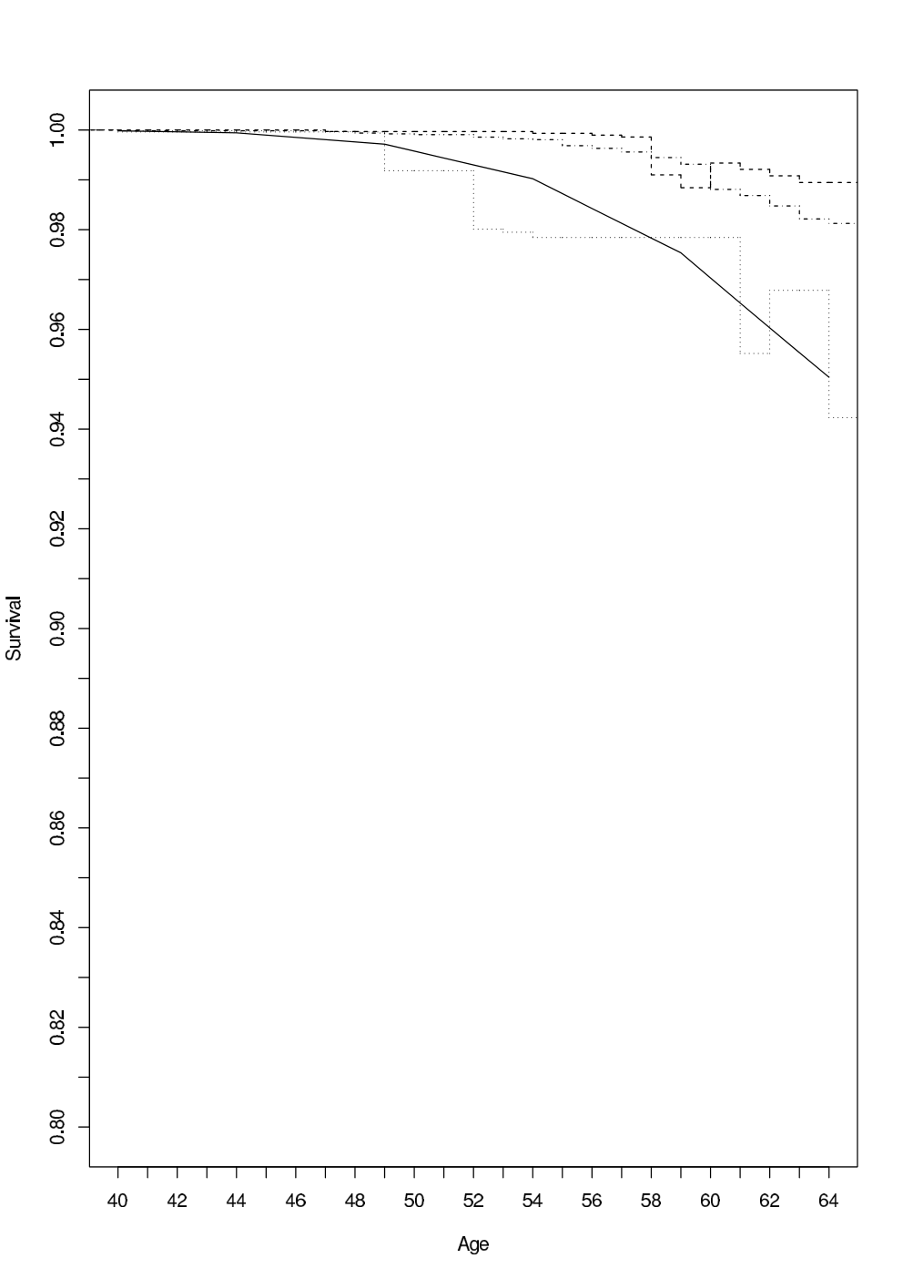
Giné, E. and Guillou, A. (2002). Rates of strong consistency for multivariate kernel density estimators. Annales de l’Institut Henri Poincaré (B) Probability and Statistics 38: 907-–922.

Schuster, E. F. (1969). Estimation of a probability density function and its derivatives. Annals of Mathematical Statistics 40: 1187–1195.

van der Vaart, A. W. (1998). Asymptotic Statistics. Cambridge University Press, Cambridge.