Geometric interpretation of the multi-scale entanglement renormalization ansatz

The multi-scale entanglement renormalization ansatz (MERA) MERA1; MERA2; MERA3; MERA4; MERA5; MERA6; MERA7 is a tensor network originally proposed as a variational ansatz for ground states of quantum spin chains that has over the years found a wider range of applications, including error correction error1; error2, machine learning machine1; machine2; machine3; machine4, statistical physics TNRyieldsMERA, holography H1; H2; dS1; dS2, and cosmology dS3; dS4. MERA spans an additional dimension, corresponding to scale, and is particularly well-suited to describe the ground state of a critical quantum spin chain, which we can think of as a lattice version of 1+1 conformal field theory (CFT). Moreover, the network of tensors resembles a discrete version of a hyperbolic geometry. Based on these and other observations Swingle conjectured H1; H2, in a pioneering contribution that initiated a fruitful, lasting interdisciplinary discussion connecting questions in quantum gravity with tensor networks H1; H2; dS1; dS2; dS3; dS4; EHM1; EHM2; HAPPY; Random1; Random2; cMERA; cMERAholo1; cMERAholo2; cMERAholo3; cMERAholo4; cMERAholo5; cMERAholo6; cMERAholo7; cMERAholo8; cMERAholo9; TNR; TNRholo1; TNRholo2; TNRholo3; TNRholo4; TNRholo5; TNRholo6, that MERA was a lattice realization of the AdS/CFT correspondence AdSCFT1; AdSCFT2; AdSCFT3. Specifically, MERA on the real line would describe a time slice of the Poincare patch of AdS₃, which corresponds to the hyperbolic plane H${}_{2}^{p}$, with line element

However, MERA is a quantum circuit that implements an entangling evolution (with time $\eta$ corresponding to the renormalization group or scale direction) and, as such, is naturally equipped with a causal structure and lorentzian signature MERA1; MERA2. This prompted Beny and several other authors, both in the context of holography dS1; dS2 and cosmology dS3; dS4, to conjecture that MERA on the real line should be interpreted instead as a Poincare patch of de Sitter spacetime dS${}_{2}^{p}$, with line element

Determining which geometry, if any, MERA may describe is thus important in order to assess the potential of this tensor network as a theoretical and numerical framework in both quantum gravity and cosmology. In this paper we establish that, when regarded as a discrete version of a CFT path integral, the geometry of MERA on the real line is that of a light sheet L${}_{2}^{p}$ with null scale direction $\eta$,

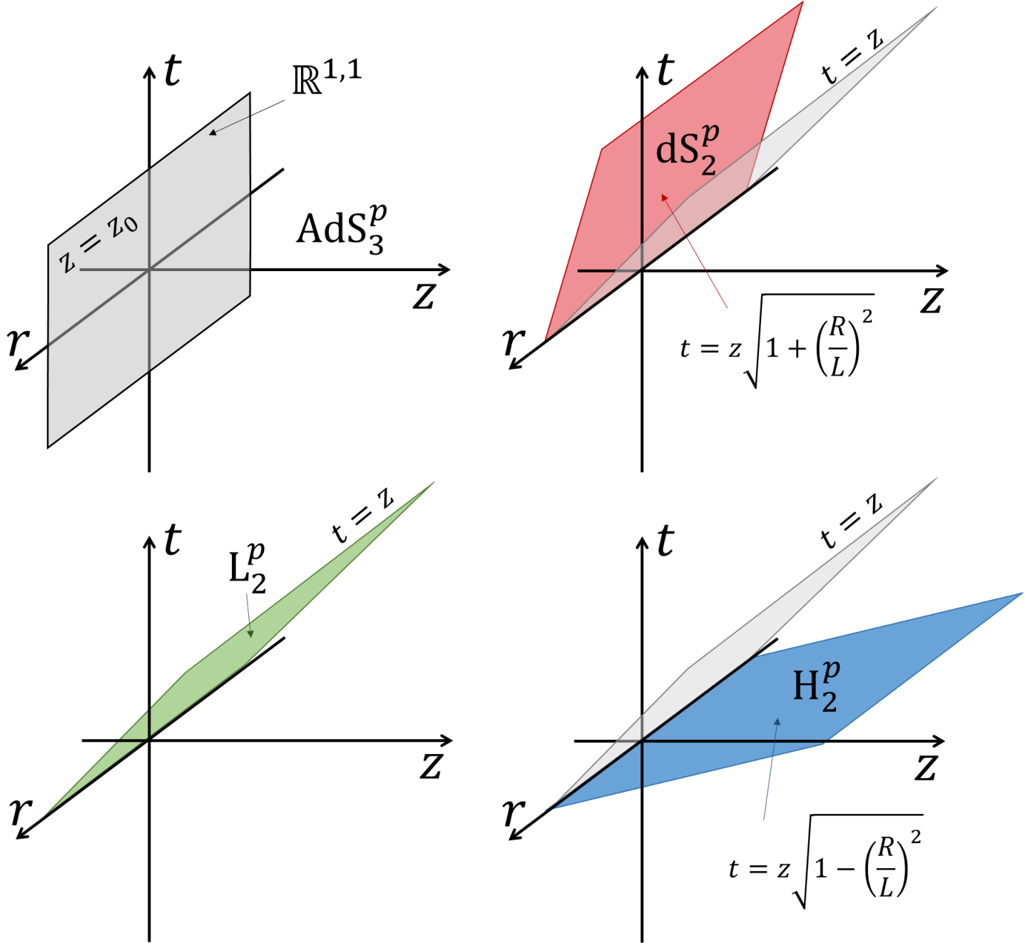
In other words, from the path integral perspective proposed in Refs. TNConfTrans; TNPathInt, MERA describes neither the hyperbolic plane nor de Sitter spacetime, but an intermediate geometry with degenerate signature, see Fig. 1. This result follows from the path integral geometry of MERA on the circle, which we determine by studying a layer $\mathcal{W}$ of MERA optimized for the ground state of a critical quantum spin chain. Specifically, we demonstrate that $\mathcal{W}$ acts on the low energy states of a periodic spin chain simply as the identity map $\mathbb{1}$, which is also the map enacted by a path integral on an annulus of a light cone L₂. In particular, $\mathcal{W}$ does not implement euclidean time evolution $e^{-\eta H}$ (nor real time evolution $e^{-i\eta H}$), as it would if it were a path integral on an annulus of the hyperbolic disk H₂ (respectively, of de Sitter spacetime dS₂).

We then propose two generalizations of MERA that may be useful toy models in holography and cosmology: (i) by interspersing layers $\mathcal{W}$ with layers of euclideons (tensors that implement euclidean time evolution $e^{-\eta H}$) we obtain a new tensor network representation of the CFT ground state corresponding to a path integral in the hyperbolic plane H₂; (ii) by interspersing layers $\mathcal{W}$ with layers of lorentzions (tensors that implement real time evolution $e^{-i\eta H}$) we produce a tensor network representation of the CFT ground state corresponding to a path integral in de Sitter spacetime dS₂.

Strategy.— Following Refs. TNConfTrans; TNPathInt, our plan is to regard the MERA network for the ground state of a critical spin chain as a discrete, approximate CFT path integral on some geometry, and to then assign that geometry to MERA. Needless to say, for this strategy to make sense, the tensor network must behave as a CFT path integral in the first place. In the continuum, the path integral on a strip defines a linear map $V:\mathcal{H}^{\mbox{\tiny CFT}}_{\mbox{\tiny in}}\rightarrow\mathcal{H}^{\mbox{\tiny CFT}}_{\mbox{\tiny out}}$ between the Hilbert spaces $\mathcal{H}^{\mbox{\tiny CFT}}_{\mbox{\tiny in}}$ and $\mathcal{H}^{\mbox{\tiny CFT}}_{\mbox{\tiny out}}$ at the boundaries $\Sigma_{\mbox{\tiny in}}$ and $\Sigma_{\mbox{\tiny out}}$ of the strip. This linear map $V$ enacts a conformal transformation that depends both on the geometry of the strip and on how we identified the two Hilbert spaces. On the other hand, a layer $\mathcal{W}$ of MERA also defines a linear map, also denoted by $\mathcal{W}$, between the Hilbert spaces of the two spin chains at its boundaries. We can then ask whether the map $\mathcal{W}$ matches the path integral map $V$ for some choice of strip geometry. It is highly non-trivial that the answer is affirmative –and not only for an optimized MERA, but also for a larger class of tensor networks described in Refs. TNConfTrans; TNPathInt).

The low energy states of a critical spin chain are in one-to-one correspondence with states of a CFT Cardy; KooSaleur; SpinChain1; SpinChain2. It is thus on these states that we want to compare the action of the linear maps $V$ and $\mathcal{W}$. In order to characterize the action of $\mathcal{W}$, we first need to explain how to relate the low energy states of the two spin chains in connects. Two difficulties lie ahead. First, in a numerical simulation of the real line (i.e. infinite critical spin chain), we do not know how to reliably compute low energy states due to the absence of a mass gap in the energy spectrum. For this reason we turn to studying finite periodic spin chains instead. Second, $\mathcal{W}$ is a coarse-graining transformation that maps states of a spin chain of size $N$ to states of a spin chain with size $N/2$. It is therefore not obvious how two identify the two Hilbert spaces, which have very different dimension. Here we will use the techniques of Refs. Cardy; KooSaleur; SpinChain1; SpinChain2; SpinChain3 to relate each low energy state in the two spin chains through their corresponding low energy state in the CFT. With this identification, we will then be ready to numerically determine the action of $\mathcal{W}$ and to finally compare it to candidate CFT linear maps $V$.

Path integral on an annulus.— We start by describing the linear map $V$ for three candidate geometries for MERA on the circle. Consider Minkowski $\mathbb{R}^{1,2}$ with metric $dl^{2}=-d{X_{0}}^{2}+d{X_{1}}^{2}+d{X_{2}}^{2}$ and the three two-dimensional manifolds given by the following constraints

see Fig. 1. We introduce polar coordinates $r=\sqrt{x^{2}+y^{2}}$ and $\theta=\arctan(y/x)$ and use the above constraints to arrive at the metrics of the hyperbolic plane H₂, the light cone L₂, and the de Sitter spacetime dS₂, namely

Notice that the light cone L₂ is the limit of small radius $R$ of both H₂ and dS₂. For simplicity we specialize to the case $r\gg R$. A standard computation Supplemental shows that the CFT path integral on an annulus with boundaries given by radial coordinate $r$ and $r/2$ produce the linear maps

where $H\equiv L_{0}+\bar{L}_{0}-c/12$ is the CFT Hamiltonian on the unit radius circle. Recall that simultaneous diagonalization of $H$ and the momentum operator $P=L_{0}-\bar{L}_{0}$,

yields energies $E_{\alpha}$ and momenta $P_{\alpha}$ that are given in terms of the CFT’s central charge $c$, scaling dimensions $\Delta_{\alpha}$ and conformal spins $S_{\alpha}$ according to CFT1; CFT2; CFT3

Map $\mathcal{W}$ between low energy states of two spin chains.— Consider now a critical spin chain Hamiltonian $H^{(\infty)}\equiv\sum_{n=\infty}^{\infty}h_{n}$ on the (discrete) real line, where $h_{n}$ is a local term that acts on a small neighbourhood of spin $n$. Following Refs. MERA5; MERA6, we obtain an approximate, scale invariant MERA representation of the ground state of $H^{(\infty)}$. The network is made of infinite layers $\mathcal{W}$ of tensors called disentanglers $u$ and isometries $w$, see Fig. 2(a). Using the same optimized tensors $u$ and $w$, we build a finite, periodic layer $\mathcal{W}$ that defines a map between two periodic chains made of $N$ and $N/2$ spins, see Fig. 2(b). The Hamiltonian $H^{(N)}\equiv\sum_{n=1}^{N}h_{n}$ on the periodic chain of size $N$ and the one-site translation operator $T^{(N)}$ can be simultaneously diagonalized,

Let $a_{\mbox{\tiny UV}}$ denote the lattice spacing, so that the radius of the periodic spin chain is $r=Na_{\mbox{\tiny UV}}/2\pi$. At low energies, after suitably normalizing $h_{n}$ normalization, the lattice Hamiltonian $H^{(N)}$ is a rescaled version of the CFT Hamiltonian $H$ Cardy, namely $H^{N}\approx H/r$, and also $P^{N}=P$, so that

We can thus identify each eigenstate $|\phi^{N}_{\alpha}\rangle$ on the lattice with a corresponding CFT state $|\phi^{\mbox{\tiny CFT}}_{\alpha}\rangle$, that is $\mbox{$|\phi^{N}_{\alpha}\rangle$}\sim\mbox{$|\phi^{\mbox{\tiny CFT}}_{\alpha}\rangle$}$. Repeating the same procedure for the spin chain of size $N/2$, we arrive at an analogous identification $\mbox{$|\phi^{N/2}_{\alpha}\rangle$}\sim\mbox{$|\phi^{\mbox{\tiny CFT}}_{\alpha}\rangle$}$, which results in an identification between the low energy states of the two spin chains,

Our goal is to then compute the matrix elements

and, by comparison with the maps in Eqs. (19)-(12), determine whether they match any of the following options

Numerical characterization of $\mathcal{W}$.— As a concrete example, we have considered the critical Ising model. Given the local Hamiltonian term $h^{\prime}_{n}=-\left(\sigma_{n}^{x}\sigma_{n+1}^{x}+\sigma_{n}^{z}\right)$, we produce a term $h_{n}$ by suitably coarse-graining $h^{\prime}_{n}$ Supplemental. In the coarse-grained spin chain, each site is described by a vector space of dimension $\chi=8$ and $h_{n}$ acts on three consecutive sites. Upon diagonalization of $H^{(N)}$ for $N=8$ sites, we obtain a number of low energy states $|\phi^{N}_{\alpha}\rangle$, which we organize Cardy; KooSaleur; SpinChain1; SpinChain2 into the identity, spin, and energy density conformal towers of the Ising CFT,

For instance, $|\mathbb{1}^{N}\rangle$ corresponds to the ground state of $H^{(N)}$, $|\sigma^{N}\rangle$ to its first excited state, and $|T^{N}\rangle$ is the (holomorphic) stress tensor state CFT1; CFT2; CFT3. Proceeding similarly with a chain of $N/2=4$ sites, we obtain analogous states $\mbox{$|\mathbb{1}^{N/2}\rangle$},\mbox{$|T^{N/2}\rangle$},\cdots$. A first numerical check confirms that $\mathcal{W}$ is indeed diagonal in these states,

in agreement with the three options (19)-(21). However, since $\mathcal{W}$ is (by construction) an isometric map, whose eigenvalues can only either vanish or be a complex phase, we have $|f_{\alpha}|=0$ or $1$, which rules out the euclidean evolution (19) corresponding to the hyperbolic disk H₂.

To discriminate between null and lorentzian evolutions, Eqs. (20) and(21), we first need to fix the arbitrary complex phase $e^{i\varphi_{\alpha}^{N}}$ in each of state $|\phi_{\alpha}^{N}\rangle$ that appears when diagonalizing the Hamiltonian $H^{(N)}$ complex, and similarly for $H^{(N/2)}$. Fortunately, we can use recently developed techniques SpinChain1; SpinChain2 based on the Koo-Saleur formula KooSaleur, which provides a lattice version $H^{(N)}\sim L_{n}+\bar{L}_{-n}$ of the Virasoro generators $L_{n}$, $\bar{L}_{-n}$ of the CFT, to establish relations between low energy states in a given conformal tower (e.g. $H_{2}^{(N)}\mbox{$|\mathbb{1}^{N}\rangle$}\approx\sqrt{c/2}\mbox{$|T^{N}\rangle$}$) and in this way eliminate relative complex phases (e.g. $e^{i(\varphi_{\mathbb{1}}^{N}-\varphi_{T}^{N})}$) within each conformal tower. Moreover, relative complex phases between different towers can be eliminated using lattice version of CFT operators SpinChain3. After carefully eliminating all these spurious complex phases Supplemental, the resulting matrix coefficients $\mathcal{W}_{\alpha\beta}$ are seen to coincide with the identity $\delta_{\alpha\beta}$, displaying no dependence on the energies $E_{\alpha}$. For instance, on the 17 lowest energy eigenstates of the Ising model, $\mathcal{W}$ acts as the identity map up to corrections below $10^{-2}$ Supplemental.

Geometric interpretation of the MERA.— We have thus numerically established that a periodic layer $\mathcal{W}$ of optimized MERA implements null time evolution on the low energy states of a periodic spin chain and therefore acts as if it was a CFT path integral on an annulus of the light cone L₂ in Eq. (8). Returning to the real line, the path integral on a strip of the geometries (1)-(3) with boundaries $\eta$ and $2\eta$, where we identify the points in two boundaries points at constant value of the new space coordinate $x\equiv rR/(a_{\mbox{\tiny UV}}\eta)$, produces the linear maps Supplemental

where now $H$ and $D$ are the CFT Hamiltonian and dilation operators on the real line Supplemental. It is well known that an infinite layer $\mathcal{W}$ of MERA implements a rescaling transformation by a scale factor $2$ MERA1; MERA2; MERA3; MERA4; MERA5; MERA6. Moreover, we have just seen on the circle that $\mathcal{W}$ does not implement time evolution. Therefore the infinite layer $\mathcal{W}$ of optimized MERA acts as $\mathcal{W}\approx 2^{iD}$, that is, as a CFT path integral on a strip of the light sheet L${}_{2}^{p}$ of Eq. (3). The presence of the dilation operator $D$ in $\mathcal{W}$ can be traced back to the identification of Hilbert spaces in the real line, which proceeds by identifying one-to-one the sites on the two infinite spin chains, in close analogy to the constant-$x$ identification in the continuum that produces the maps (26)-(28) Supplemental. Notice that on the circle, a one-to-one identification between sites was not possible due to the different sizes $N$ and $N/2$ of the spin chains, and we had to use instead the low energy spectrum identification, in close analogy to the constant-$\theta$ identification in the continuum that produces instead the maps (10)-(12).

Euclidean and lorentzian MERA.— Having numerically established the linear map implemented by a layer $\mathcal{W}$ of optimized MERA, we can now modify the tensor network so that it implements other maps and in this way reproduce CFT path integrals on other geometries. For instance, an infinite layer $\mathcal{W}_{+}\equiv\mathcal{W}\mathcal{T}$ obtained by pre-multiplying $\mathcal{W}$ by a transfer matrix $\mathcal{T}$ made of a row of euclideons $e$, where $\mathcal{T}$ implements an euclidean time evolution $e^{-H}$ TNConfTrans; TNPathInt, results in the linear map $V_{\mbox{\tiny H${}_{2}^{p}$}}$ of Eq. (26), thus corresponding to a path integral on a strip of the hyperbolic plane H${}_{2}^{p}$ (and similarly on the circle with map $V_{\mbox{\tiny H${}_{2}$}}$ of Eq. (10), corresponding to a path integral on an annulus of the hyperbolic disk H₂). The resulting construction in Fig. 3(a), that we call euclidean MERA, closely realizes the scenario, envisaged by Swingle H1; H2, of a tensor network that represents a time slice of AdS₃. In turn, a lorentzian MERA is obtained using instead layers $\mathcal{W}_{-}\equiv\mathcal{W}\mathcal{T}^{\prime}$, see Fig. 3(b), where $\mathcal{T}^{\prime}$ is made of a row of lorentzions $l$ and implements a lorentzian time evolution $e^{-iH}$ Supplemental. $\mathcal{W}_{-}$ is then seen to implement the linear map $V_{\mbox{\tiny dS${}_{2}^{p}$}}$ of Eq. (28), thus corresponding to a path integral on a strip of the Poincare de Sitter spacetime dS${}_{2}^{p}$ (and similarly on the circle), thus closely realizing the scenario, envisaged by Cedric and other authors dS1; dS2; dS3; dS4, of a tensor network that represents de Sitter spacetime.

Discussion.— In this work we have assigned a path integral geometry to the (null, euclidean, and lorentzian) MERA starting from three candidate geometries and enforcing only rule 1 of Ref. TNPathInt, which demands “consistency between the path integral map $V$ and the tensor network map $\mathcal{W}$”. However, a local rescaling $g_{\mu\nu}(\eta,r)\rightarrow g^{\prime}_{\mu\nu}(\eta,r)=\Omega(\eta,r)^{2}g_{\mu\nu}(\eta,r)$ in a CFT leaves the map $V$ essentially unchanged, so that a geometric assignment based on rule 1 of Ref. TNPathInt alone only determines the conformal class of the metric $g_{\mu\nu}$. However, we can now fix the scale factor $\Omega(\eta,r)$ and recover the geometries in Eqs. 1-3 and 7-9 (that is, without preassuming them as candidates) by enforcing rule 2 of Ref. TNPathInt, which states that “the lattice spacing is the same constant $a_{\mbox{\tiny UV}}$ throughout the tensor network” Supplemental.

In summary, we have numerically established that a MERA optimized to represent the ground state of a critical quantum spin chain on the circle / real line behaves as a CFT path integral on a light cone / light sheet geometry. Moreover, we have proposed two new tensor networks that correspond to hyperbolic space and de Sitter spacetime, thus realizing previously conjectured constructions. Particularly intriguing is the optimized MERA refusal to perform real time evolution (something that is in principle possible within the MERA variational class), suggesting that the optimal preparation of a CFT ground state through a path integral TNRholo1; TNRholo2; TNRholo3; TNRholo4; TNRholo5; TNRholo6; complexity1; complexity2; complexity3; complexity4 does not actually require time evolution Sully. Perhaps even more tantalizing is the fact that the tensor networks discussed above open a new venue to numerically simulate quantum field theories in curved spacetime Adam.

Acknowledgments. The authors thank Bartlomiej Czech, Pawel Caputa, Olalla Castro-Alvaredo, William Donnelly, Benjamin Doyon, Davide Gaiotto, Qi Hu, Lampros Lamprou, Juan Maldacena, David Mateos, Samuel McCandlish, James Sully, Vasudev Shyam, Tadashi Takayanagi, and Xiao-liang Qi for fruitful discussions and feedback. Very special thanks go to Ling-Yan (Janet) Hung and Rob Myers for their patient, tenacious attempt to teach us CFT and curved spacetime background material. The authors acknowledge support by the Simons Foundation (Many Electron Collaboration), by NSERC (discovery grant), and by Compute Canada. Research at Research at Perimeter Institute is supported by the Government of Canada through the Department of Innovation, Science and Economic Development Canada and by the Province of Ontario through the Ministry of Research, Innovation and Science.

References

- (1) G. Vidal, Entanglement renormalization, Phys. Rev. Let. 99, 220405 (2007), arXiv:cond-mat/0512165.
- (2) G. Vidal, A class of quantum many-body states that can be efficiently simulated, Phys. Rev. Lett. 101, 110501 (2008), arXiv:quant-ph/0610099.
- (3) G. Evenbly, G. Vidal, Algorithms for entanglement renormalization Phys. Rev. B 79 (14), 144108 (2009), arXiv:0707.1454.
- (4) V. Giovannetti, S. Montangero, R. Fazio Quantum Multiscale Entanglement Renormalization Ansatz Channels Phys. Rev. Lett. 101, 180503 (2009), arXiv:0804.0520.
- (5) R. N. C. Pfeifer, G. Evenbly, G. Vidal Entanglement renormalization, scale invariance, and quantum criticality, Phys. Rev. A 79(4), 040301(R) (2009), arXiv:0810.0580.
- (6) G. Evenbly, G. Vidal, Quantum Criticality with the Multi-scale Entanglement Renormalization Ansatz, chapter 4 of ”Strongly Correlated Systems. Numerical Methods” (Springer Series in Solid-State Sciences, Vol. 176 2013), arXiv:1109.5334
- (7) M. Aguado, G. Vidal Entanglement renormalization and topological order, Phys. Rev. Lett. 100, 070404 (2008), arXiv:0712.0348
- (8) A. J. Ferris, D. Poulin Tensor Networks and Quantum Error Correction, Phys. Rev. Lett. 113, 030501(2014), arXiv:1312.4578.
- (9) A.J. Ferris, D. Poulin, Branching MERA codes: A natural extension of classical and quantum polar codes, Information Theory (ISIT), 2014 IEEE International Symposium on, 1081-1085.
- (10) C. Beny, Deep learning and the renormalization group, arXiv:1301.3124
- (11) E.M. Stoudenmire, D.J. Schwab Supervised Learning with Quantum-Inspired Tensor Networks, Advances in Neural Information Processing Systems 29, 4799 (2016), arXiv:1605.05775.
- (12) Y. Levine, O. Sharir, N. Cohen, A. Shashua, Bridging Many-Body Quantum Physics and Deep Learning via Tensor Networks, arXiv:1803.09780.
- (13) I. Cong, S. Choi, M. D. Lukin, Quantum Convolutional Neural Networks, arXiv:1810.03787
- (14) G. Evenbly, G. Vidal Tensor network renormalization yields the multi-scale entanglement renormalization ansatz, Phys. Rev. Lett. 115, 200401 (2015), arXiv:1502.05385
- (15) B. Swingle, Entanglement Renormalization and Holography, Phys. Rev. D 86, 065007 (2012), arXiv:0905.1317.
- (16) B. Swingle, Constructing holographic spacetimes using entanglement renormalization, arXiv:1209.3304.
- (17) C. Beny, Causal structure of the entanglement renormalization ansatz, New J. Phys. 15 (2013) 023020, arXiv:1110.4872.
- (18) B. Czech, L. Lamprou, S.l McCandlish, and J. Sully, Tensor Networks from Kinematic Space, JHEP07 (2016) 100, arXiv:1512.01548.
- (19) R.S. Kunkolienkar, K. Banerjee, Towards a dS/MERA correspondence, Int. J. Mod. Phys. D 26, 1750143 (2017), arXiv:1611.08581.
- (20) N. Bao, C. Cao, S. M. Carroll, A. Chatwin-Davies, De Sitter space as a tensor network: Cosmic no-hair, complementarity, and complexity, Phys. Rev. D 96, 123536 (2017), arXiv:1709.03513.
- (21) X.-L. Qi, Exact holographic mapping and emergent spacetime geometry, arXiv:1309.6282.
- (22) C. H. Lee, X.-L. Qi Exact holographic mapping in free fermion systems, Phys. Rev. B 93,035112 (2016), arXiv:1503.08592.
- (23) F. Pastawski, B. Yoshida, D. Harlow, J. Preskill, Holographic quantum error-correcting codes: Toy models for the bulk/boundary correspondence, JHEP 06 (2015) 149, arXiv:1503.06237.
- (24) P. Hayden, S. Nezami, X.-L. Qi, N. Thomas, M. Walter, Z. Yang, Holographic duality from random tensor networks, JHEP 11 (2016) 009, arXiv:1601.01694.
- (25) X.-L. Qi, Z. Yang, Space-time random tensor networks and holographic duality, arXiv:1801.05289.
- (26) J. Haegeman, T. J. Osborne, H. Verschelde and F. Verstraete, Entanglement Renormalization for Quantum Fields in Real Space, Phys. Rev. Lett., 110, 100402 (2013), arxiv:1102.5524
- (27) A. Mollabashi, M. Naozaki, S. Ryu and T. Takayanagi, Holographic geometry of cMERA for quantum quenches and finite temperature, JHEP (2014) 2014: 98, arxiv:1311.6095.
- (28) M. Nozaki, S. Ryu and T. Takayanagi, Holographic geometry of entanglement renormalization in quantum field theories, JHEP (2012) 2012: 10, arxiv:1208.3469.
- (29) J. Molina-Vilaplana, Information geometry of entanglement renormalization for free quantum fields, JHEP (2015) 2015:2 (mar, 2015), arxiv:1503.07699.
- (30) J. Molina-Vilaplana, Entanglement renormalization and two dimensional string theory, Phys. Lett. B 755 (2016) 421-425, arxiv:1510.09020.
- (31) M. Miyaji, S. Ryu, T. Takayanagi and X. Wen, Boundary states as holographic duals of trivial spacetimes, JHEP (2015) 2015: 152, arxiv:1412.6226.
- (32) M. Miyaji, T. Numasawa, N. Shiba, T. Takayanagi, K. Watanabe, cMERA as Surface/State Correspondence in AdS/CFT, Phys. Rev. Lett. 115, 171602 (2015), arXiv:1506.01353.
- (33) M. Miyaji and T. Takayanagi, Surface/state correspondence as a generalized holography, Progress of Theoretical and Experimental Physics 2015 (mar, 2015) , arxiv:1503.03542.
- (34) X. Wen, G. Y. Cho, P. L. S. Lopes, Y. Gu, X. L. Qi and S. Ryu, Holographic entanglement renormalization of topological insulators, Phys. Rev. B 94, 075124 (2016), arxiv:1605.07199.
- (35) J. R. Fliss, R. G. Leigh and O. Parrikar, Unitary Networks from the Exact Renormalization of Wave Functionals, Phys. Rev. D 95, 126001 (2017), arxiv:1609.03493.
- (36) G. Evenbly, G. Vidal, Tensor network renormalization, Phys. Rev. Lett. 115 (18), 180405 (2015), arXiv:1412.0732.
- (37) M. Miyaji, T. Takayanagi, K. Watanabe, From Path Integrals to Tensor Networks for AdS/CFT, Phys. Rev. D 95, 066004 (2017), arXiv:1609.04645.
- (38) P. Caputa, N. Kundu, M. Miyaji, T. Takayanagi, K. Watanabe, Anti-de Sitter Space from Optimization of Path Integrals in Conformal Field Theories, Phys. Rev. Lett. 119, 071602 (2017), arXiv:1703.00456.
- (39) P. Caputa, N. Kundu, M. Miyaji, T. Takayanagi, K. Watanabe, Liouville Action as Path-Integral Complexity: From Continuous Tensor Networks to AdS/CFT, JHEP 11(2017)097, arXiv:1706.07056.
- (40) B. Czech, Einstein’s equations from Varying Complexity, Phys. Rev. Lett. 120, 031601 (2018), arXiv:1706.00965.
- (41) P. Caputa, J. M. Magan, Quantum Computation as Gravity, arXiv:1807.04422.
- (42) T. Takayanagi, Holographic Spacetimes as Quantum Circuits of Path-Integrations, arXiv:1808.09072
- (43) J.M. Maldacena, The Large N Limit of Superconformal Field Theories and Supergravity, Adv. Theor. Math. Phys. 2:231-252 (1998), arXiv:hep-th/9711200.
- (44) S. S. Gubser, I. R. Klebanov, and A. M. Polyakov, Gauge Theory Correlators from Non-Critical String Theory, Phys. Lett. B 428, 105 (1998), arXiv:hep-th/9802109.
- (45) E. Witten, Anti De Sitter Space And Holography, Adv. Theor. Math. Phys. 2, 253 (1998), arXiv:hep-th/9802150.
- (46) A. Milsted, G. Vidal, Tensor networks as conformal transformations, arXiv:1805.12524
- (47) A. Milsted, G. Vidal, Tensor networks as path integral geometry, arXiv:1807.02501
- (48) J. L. Cardy, Conformal invariance and universality in finite-size scaling, J. Phys. A: Math. Gen. 17, L385 (1984).
- (49) W. M. Koo and H. Saleur, Representations of the Virasoro algebra from lattice models, Nucl. Phys. B 426, 459 (1994), arXiv:hep-th/9312156.
- (50) A. Milsted, G. Vidal, Extraction of conformal data in critical quantum spin chains using the Koo-Saleur formula, Phys. Rev. B 96, 245105 (2017), arXiv:1706.01436
- (51) Y. Zou, A. Milsted, G. Vidal, Conformal data and renormalization group flow in critical quantum spin chains using periodic uniform matrix product states, arXiv:1710.05397
- (52) Y. Zou, A. Milsted, G. Vidal, Conformal fields and operator product expansion in critical quantum spin chains, In preparation.
- (53) G. Evenbly, Algorithms for tensor network renormalization Phys. Rev. B 95, 045117 (2017), arXiv:1509.07484.
- (54) G. Evenbly, G. Vidal Local scale transformations on the lattice with tensor network renormalization, Phys. Rev. Lett. 116, 040401 (2016), arXiv:1510.00689.
- (55) P. Ginsparg, Applied Conformal Field Theory, arXiv:hep-th/9108028 (1988).
- (56) P. Di Francesco, P. Mathieu, and D. Senechal, Conformal Field Theory (Springer, New York, 2012).
- (57) M. Henkel, Conformal Invariance and Critical Phenomena, (Springer, New York, 1999).
- (58) See appendices below for further details.
- (59) The local Hamiltonian term is normalized (by a constant shift and a rescaling, , where the constants and are independent of the size of the spin chain) such that the low energy spectrum matches that of a CFT on a circle of length , or radius , where is the lattice spacing.
- (60) If is a normalized eigenstate of , with , then so is for any angle . Therefore by diagonalizing we obtain (normalized) energy eigenvectors that are only defined up to an arbitrary complex phase .
- (61) D. Stanford, L. Susskind, Complexity and shock wave geometries, Phys. Rev. D 90, 126007 (2014), arxiv:1406.2678.
- (62) A. R. Brown, D. A. Roberts, L. Susskind, B. Swingle, Y. Zhao, Complexity, action, and black holes, Phys. Rev. D 93, 086006 (2016), arxiv:1512.04993.
- (63) A. R. Brown, D. A. Roberts, L. Susskind, B. Swingle, Y. Zhao, Holographic complexity equals bulk action?, Phys. Rev. Lett. 116, 191301 (2016), arxiv:1509.07876.
- (64) R. Jefferson, R. C. Myers, Circuit complexity in quantum field theory, JHEP10(2017)107, arXiv:1707.08570
- (65) S. Chapman, J. Eisert, L. Hackl, M. P. Heller, R. Jefferson, H. Marrochio, R. C. Myers, Complexity and entanglement for thermofield double states, arXiv:1810.05151
- (66) J. Sully, R. Myers, G. Vidal, The true truth about CFT complexity, in eternal preparation.
- (67) A. Lewis, Q. Hu, G. Vidal, Tensor networks for quantum field theories in curved spacetime, in preparation.
I Appendix: MERA on the circle
In this Appendix we review how to assign a path integral geometry to the periodic MERA, which is a tensor network used to represent the ground state of a critical quantum spin chain on the circle. We consider both the usual MERA (in what follows named null MERA) as well as the two extensions proposed in the main text, namely the euclidean MERA and the lorentzian MERA, see Fig. 4. We have argued that, from a path integral perspective, the periodic version of these tensor networks represent the following geometries: