Qubit positive-operator-valued measurements by destructive weak measurements

In earlier work Varbanov and Brun 2007, it was shown that a generalized measurement can be decomposed into a series of stochastic processes such that the trajectory corresponds to a random walk in a simplex. Here we use a similar approach to parametrize the measurement operator during the sequence of weak measurements. The intuition is to map the current POVM element at each step of a sequence of weak measurements into a convex combination of the original POVM elements. We will show that, for a linearly independent POVM, the conditions to perform a measurement where each outcome corresponds to a vector in the simplex can be satisfied.

To decompose a linearly independent POVM into stochastic processes of weak measurements, we use a family of measurement operators $M(\vec{x})$ of the form

$$M(\vec{x})=f(\vec{x})U(\vec{x})\sqrt{\sum^{n}_{i=1}x_{i}E_{i}},$$

(18)

where $U(\vec{x})$ is a unitary operator, $f(\vec{x})$ is a normalization factor, and

$$\vec{x}\in\triangle^{n-1}=\left\{(x_{1},\cdots,x_{n})|\sum^{n}_{i=1}x_{i}=1,\ x_{i}\geq 0\ \forall i\right\}.$$

(19)

The form of Eq. (18) is fairly general because any matrix allows for a polar decomposition, and Eq. (18) only requires the positive-semidefinite matrix to be the square root of a linear combination of the POVM elements. The vector $\vec{x}$ characterizes the position of the random walk in the $(n-1)$-simplex, $\triangle^{n-1}$. Note that for a given position $\vec{x}$ in the walk,

$$M^{\dagger}(\vec{x})M(\vec{x})\propto\sum^{n}_{i=1}x_{i}E_{i}.$$

(20)

This form characterizes how the POVM element of the weak measurement evolves as a convex combination of the original POVM elements. It will be shown in Sec. V that $\vec{x}$ will approach one of the vertices of $\triangle^{n-1}$ after many measurements: $\vec{x}\to(\cdots,0,1,0,\cdots)$. The vertex corresponds to the outcome $E_{j}$ of this POVM $\{E_{i}\}^{n}_{i=1}$. An example of performing a 3-outcome POVM is shown in Fig. 1.

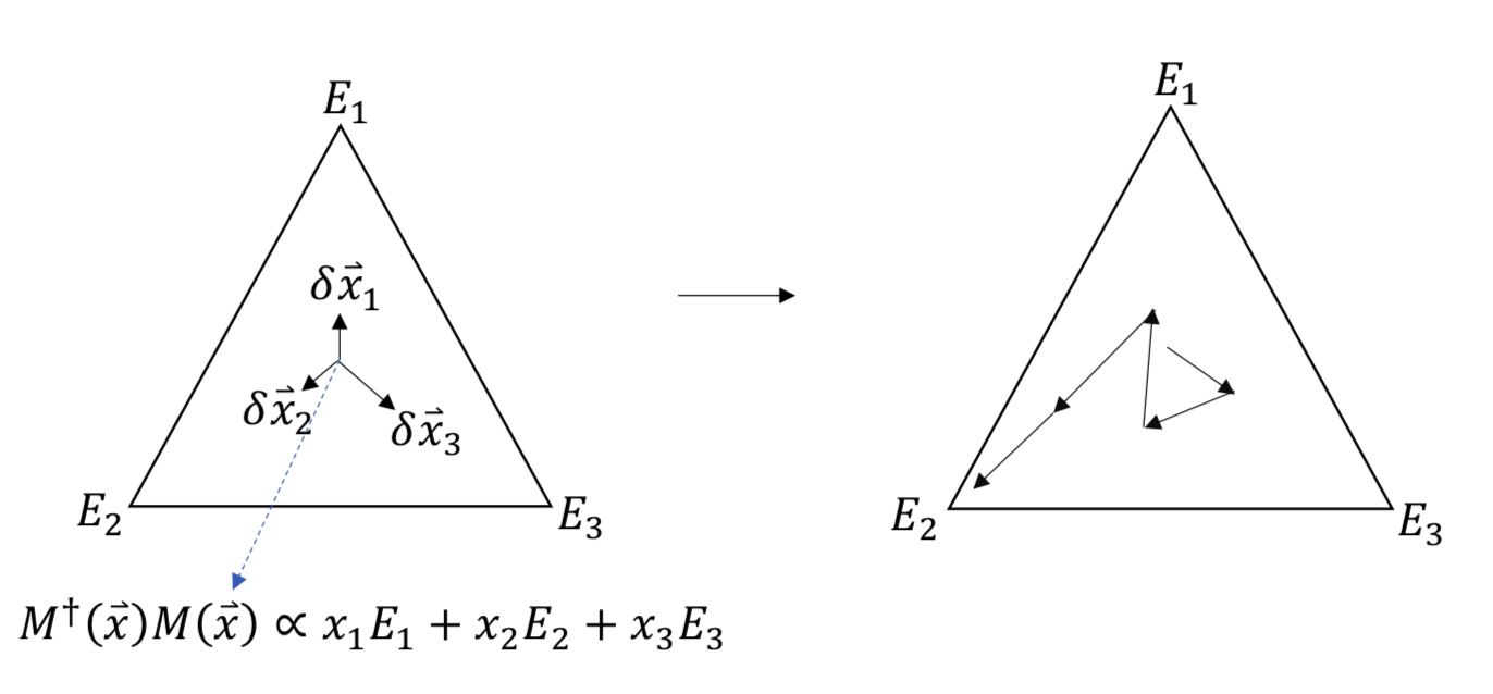
Before making any measurement, $\vec{x}$ is at the middle of $\triangle^{n-1}$, so the random walk starts from

$$\vec{x}=\vec{x}_{0}=\frac{1}{n}\left(\begin{array}[]{c}1\\ \vdots\\ 1\end{array}\right),$$

(21)

and $M(\vec{x}_{0})=U(\vec{x}_{0})=I$. After each weak measurement is made, the new position $\vec{x}$ remains in $\triangle^{n-1}$ if the weak measurement, with measurement operators $\{M_{k}(\vec{x})\}^{n}_{k=1}$ satisfying

$$\sum^{n}_{k=1}M^{\dagger}_{k}(\vec{x})M_{k}(\vec{x})=I,$$

(22)

satisfies

$$M^{\dagger}(\vec{x})M^{\dagger}_{k}(\vec{x})M_{k}(\vec{x})M(\vec{x})\propto M^{\dagger}(\vec{x}_{k})M(\vec{x}_{k})$$

(23)

for each outcome $k$ such that

$$\vec{x}_{k}\in\triangle^{n-1}.$$

(24)

Note that $\vec{x}_{k}$ is a new position in the simplex $\triangle^{n-1}$ after outcome $k$, and $\delta\vec{x}_{k}\equiv\vec{x}_{k}-\vec{x}$ is expected to be a small quantity given that we are performing weak measurements. Using Eq. (18) for $M(\vec{x})$, we can rewrite Eq. (23) as

		$\displaystyle\sqrt{\sum^{n}_{i=1}x_{i}E_{i}}U^{\dagger}(\vec{x})M^{\dagger}_{k}(\vec{x})M_{k}(\vec{x})U(\vec{x})\sqrt{\sum^{n}_{i=1}x_{i}E_{i}}$
		$\displaystyle\propto\sum^{n}_{i=1}(\vec{x}_{k})_{i}E_{i}.$		(25)

Define a new set of POVM elements by

$$E_{i}(\vec{x})\equiv U(\vec{x})E_{i}U^{\dagger}(\vec{x}),\ \ \forall\ i\in\{1,\cdots,n\}.$$

(26)

It can be easily checked that $\{E_{i}\}^{n}_{i=1}$ is linearly independent if and only if $\{E_{i}(\vec{x})\}^{n}_{i=1}$ is linearly independent. Inserting Eq. (26) back into Eq. (IV.1), we have

		$\displaystyle M^{\dagger}_{k}(\vec{x})M_{k}(\vec{x})\propto$
		$\displaystyle\left(\sum^{n}_{i=1}x_{i}E_{i}(\vec{x})\right)^{-\frac{1}{2}}\left(\sum^{n}_{i=1}(\vec{x}_{k})_{i}E_{i}(\vec{x})\right)\left(\sum^{n}_{i=1}x_{i}E_{i}(\vec{x})\right)^{-\frac{1}{2}}.$		(27)

We can expand all the operators as linear combinations of Pauli operators and the identity; i.e., for each $i$,

$$E_{i}(\vec{x})=q_{i}(I+\vec{v}_{i}\cdot\vec{\sigma}),$$

(28)

where $\vec{\sigma}$ is the vector of Pauli matrices and $q_{i}$, $\vec{v}_{i}$ are the expansion coefficients. By assumption, all $q_{i}$’s are strictly positive. For convenience, the indication of $\vec{x}$ dependence for $q_{i}$ and $\vec{v}_{i}$ have been dropped. We have

	$\displaystyle\sum^{n}_{i=1}x_{i}E_{i}(\vec{x})$	$\displaystyle=\sum^{n}_{i=1}x_{i}q_{i}I+\sum^{n}_{i=1}x_{i}q_{i}\vec{v}_{i}\cdot\vec{\sigma}$
		$\displaystyle\propto I+\frac{1}{\sum^{n}_{i=1}x_{i}q_{i}}\left(\sum^{n}_{i=1}x_{i}q_{i}\vec{v}_{i}\right)\cdot\vec{\sigma}$
		$\displaystyle=I+\vec{r}\cdot\vec{\sigma},$		(29)

where

$$\vec{r}\equiv\frac{1}{\sum^{n}_{i=1}x_{i}q_{i}}\left(\sum^{n}_{i=1}x_{i}q_{i}\vec{v}_{i}\right).$$

(30)

Using the property shown in Appendix A, the inverse square root of Eq. (IV.1) is

$$\left(\sum^{n}_{i=1}x_{i}E_{i}(\vec{x})\right)^{-\frac{1}{2}}\propto\left(I+\vec{r}\cdot\vec{\sigma}\right)^{-\frac{1}{2}}\propto(I-b\vec{r}\cdot\vec{\sigma}),$$

(31)

where

$$b=\frac{1-\sqrt{1-|\vec{r}|^{2}}}{|\vec{r}|^{2}}.$$

(32)

Similarly, we can write

$$\sum^{n}_{i=1}(\vec{x}_{k})_{i}E_{i}(\vec{x})\propto I+\vec{r}_{k}\cdot\vec{\sigma},$$

(33)

where

$$\vec{r}_{k}\equiv\frac{1}{\sum^{n}_{i=1}(\vec{x}_{k})_{i}q_{i}}\left(\sum^{n}_{i=1}(\vec{x}_{k})_{i}q_{i}\vec{v}_{i}\right),$$

(34)

and define $\delta\vec{r}_{k}\equiv\vec{r}_{k}-\vec{r}$. Inserting Eqs. (31) and (33) to Eq. (IV.1), the condition becomes

	$\displaystyle M^{\dagger}_{k}(\vec{x})M_{k}(\vec{x})$	$\displaystyle\propto(I-b\vec{r}\cdot\vec{\sigma})\left(I+\vec{r}_{k}\cdot\vec{\sigma}\right)(I-b\vec{r}\cdot\vec{\sigma})$		(35)
		$\displaystyle\propto I+\frac{b(\vec{r}\cdot\delta\vec{r}_{k})\vec{r}+(\frac{1}{b}-1)\delta\vec{r}_{k}}{1-\vec{r}\cdot\vec{r}_{k}}\cdot\vec{\sigma}.$		(36)

The transformation from Eq. (35) to Eq. (36) is by the properties of Pauli matrices and $1-2b+b^{2}|\vec{r}|^{2}=0$ from Eq. (32). Hence,

		$\displaystyle M^{\dagger}_{k}(\vec{x})M_{k}(\vec{x})=$
		$\displaystyle c_{k}\left[\left(1-\vec{r}\cdot\vec{r}_{k}\right)I+\left(b(\vec{r}\cdot\delta\vec{r}_{k})\vec{r}+(\frac{1}{b}-1)\delta\vec{r}_{k}\right)\cdot\vec{\sigma}\right],$		(37)

where the $c_{k}$’s are $positive$ constants to be determined. The condition to be a measurement,

$$\sum^{n}_{k=1}M^{\dagger}_{k}(\vec{x})M_{k}(\vec{x})=I,$$

(38)

requires

$\displaystyle\left\{\begin{array}[]{l}\displaystyle\sum^{n}_{k=1}c_{k}(1-|\vec{r}|^{2})-\displaystyle\sum^{n}_{k=1}c_{k}\delta\vec{r}_{k}\cdot\vec{r}=1,\\ b\left(\vec{r}\cdot\displaystyle\sum^{n}_{k=1}c_{k}\delta\vec{r}_{k}\right)\vec{r}+\left(\frac{1}{b}-1\right)\displaystyle\sum^{n}_{k=1}c_{k}\delta\vec{r}_{k}=0.\end{array}\right.$

It is sufficient to solve the following conditions,

$\displaystyle\left\{\begin{array}[]{l}\displaystyle\sum^{n}_{k=1}c_{k}=\frac{1}{1-|\vec{r}|^{2}},\\ \displaystyle\sum^{n}_{k=1}c_{k}\delta\vec{r}_{k}=0.\end{array}\right.$

Note that $|\vec{r}|$ cannot be 1 because $|\vec{r}|=1$ happens only if the $E_{i}$’s are $all$ proportional to the $same$ projector, but this contradicts the assumption that the $E_{i}$’s are linearly independent.

The question now becomes whether there exists a set of $c_{k}$’s ($>0$) and $\vec{x}_{k}$’s ($\in\triangle^{n-1}$) such that Eq. (IV.1) is satisfied. First of all, $\sum^{n}_{i=1}E_{i}(\vec{x})=I$ implies that

$$\vec{q}=(q_{1},\cdots,q_{n})\in\triangle^{n-1}\ \ \text{and}\ \ \sum^{n}_{i=1}q_{i}\vec{v}_{i}=0.$$

(45)

The $\vec{v}_{i}$’s and $\vec{r}$ are 3-dimensional Bloch vectors and $\vec{x}$ is an n-dimensional vector in $\triangle^{n-1}$, where $n$ can only be 2, 3 or 4 in our case. It is shown in Appendix B that there is a one-to-one map between $\triangle^{n-1}$ and the “allowed” space of $\vec{r}$, denoted as $\triangle^{\vec{r}}$,

$$\triangle^{\vec{r}}\equiv\{\vec{r}\mid\vec{r}=\frac{1}{\vec{x}\cdot\vec{q}}\left(\sum^{n}_{i=1}x_{i}q_{i}\vec{v}_{i}\right),\ \forall\vec{x}\in\triangle^{n-1}\}.$$

(46)

For $n=2$, $\triangle^{1}$ is a line and $\triangle^{\vec{r}}$ is a line spanned by a pair of parallel and opposite-directioned vectors $\vec{v}_{1,2}$; for $n=3$, $\triangle^{2}$ is a regular triangle and $\triangle^{\vec{r}}$ is a 2-D triangle stretched by $\vec{v}_{1,2,3}$; for $n=4$, $\triangle^{3}$ is a regular tetrahedron and $\triangle^{\vec{r}}$ is a tetrahedron stretched by $\vec{v}_{1,2,3,4}$. An example of the $n=3$ case is illustrated in Fig. 2. Note that the $\vec{v}_{i}$’s are $E_{i}(\vec{x})$’s Bloch vectors, which are rotated from the Bloch vectors of the original $E_{i}$’s.

It is clear that there are many solutions to Eq. (IV.1); one simple solution is

$\displaystyle\left\{\begin{array}[]{l}c_{k}=\frac{1}{n(1-|\vec{r}|^{2})},\ \ \ \ \forall k\in\{1,\cdots,n\},\\ \displaystyle\sum^{n}_{k=1}\delta\vec{r}_{k}=0,\end{array}\right.$

where the $\delta\vec{r}_{k}=\vec{r}_{k}-\vec{r}$ are vectors lying in $\triangle^{\vec{r}}$. For example, when $n=3$, the three vectors $\delta\vec{r}_{k}$’s lie in a triangle and add up to zero vector. The three $\delta\vec{r}_{k}$’s are given by three $\vec{r}_{k}$’s, which correspond to three $\vec{x}_{k}$’s in $\triangle^{n-1}$. In fact, we can solve for the set of $\vec{x}_{k}$’s if and only if we can solve for the set of $\delta\vec{r}_{k}$’s.

So far we have shown that it is possible to perform a weak measurement while staying in a simplex. However, it was assumed that we can choose arbitrary sets of $\vec{x}_{k}$’s, which correspond to arbitrary weak measurements. We now show that even using a more restricted class of weak measurements—destructive weak measurement—Eq. (IV.1) still can be satisfied. Therefore we can perform a series of destructive weak measurements such that it corresponds to a random walk in a simplex. However, the choice of $\delta\vec{r}_{k}$’s in Eq. (IV.1) are more restricted in this case.

In Sec. II, we reintroduced the model of destructive weak measurements in Chen and Brun 2018. It consists of coupling the system with an ancilla qubit in state $|0\rangle$ by a weak swap operation, followed by a projective POVM on the ancilla. The outcome $\hat{P}_{k}=s_{k}|e_{k}\rangle\langle e_{k}|$ of this projective POVM corresponds to a measurement operator

$\displaystyle M_{k}=\sqrt{s_{k}}\left(\begin{array}[]{cc}\langle e_{k}|0\rangle e^{-i\phi}&-i\langle e_{k}|1\rangle\sin\phi\\ 0&\langle e_{k}|0\rangle\cos\phi\end{array}\right)$

on the system. From the other direction, as shown in Chen and Brun 2018, for a set of eigenvectors $\{|b_{k}\rangle,|\overline{b_{k}}\rangle\}$ of $M^{\dagger}_{k}M_{k}$, where

$$|b_{k}\rangle=\alpha_{k}|0\rangle+\beta_{k}e^{i\chi_{k}}|1\rangle,\ \ |\overline{b_{k}}\rangle=\beta_{k}|0\rangle-\alpha_{k}e^{i\chi_{k}}|1\rangle,$$

(53)

and

$$\alpha_{k},\beta_{k}\geq 0,\ \ \alpha_{k}^{2}+\beta^{2}_{k}=1,\ \ \chi_{k}\in\mathbb{R},$$

(54)

there exists a corresponding vector $|e_{k}\rangle$ of $\hat{P}_{k}$ on the ancilla that will give us those eigenvectors. With this $|e_{k}\rangle$, the eigenvalues of $M^{\dagger}_{k}M_{k}$ take the form

$$\lambda_{k},\overline{\lambda}_{k}=\frac{1}{2}s_{k}\left(1+\frac{\sqrt{1-4\alpha_{k}^{2}\beta^{2}_{k}}\cos^{2}\phi\pm\sin^{2}\phi}{\sqrt{1-4\alpha^{2}_{k}\beta^{2}_{k}\cos^{2}\phi}}\right).$$

(55)

On the other hand, one can check that if $\sum^{n}_{k=1}M^{\dagger}_{k}M_{k}=I$ then the corresponding $\hat{P}_{k}$’s on the ancilla form a projective POVM.

This result can be translated into the Bloch sphere picture for $M^{\dagger}_{k}M_{k}$:

	$\displaystyle M^{\dagger}_{k}M_{k}$	$\displaystyle=\lambda_{k}|b_{k}\rangle\langle b_{k}|+\overline{\lambda}_{k}|\overline{b_{k}}\rangle\langle\overline{b_{k}}|$
		$\displaystyle=\frac{\left(\lambda_{k}+\overline{\lambda}_{k}\right)}{2}\left(I+\frac{\lambda_{k}-\overline{\lambda}_{k}}{\lambda_{k}+\overline{\lambda}_{k}}\hat{n}_{k}\cdot\vec{\sigma}\right),$		(56)

where the unit vector $\hat{n}_{k}$ is

$\displaystyle\hat{n}_{k}=\left(\begin{array}[]{c}2\alpha_{k}\beta_{k}\cos\chi_{k}\\ -2\alpha_{k}\beta_{k}\sin\chi_{k}\\ \alpha^{2}_{k}-\beta^{2}_{k}\end{array}\right).$

The explicit expression for $M^{\dagger}_{k}M_{k}$ is

		$\displaystyle M^{\dagger}_{k}M_{k}=\frac{s_{k}}{2}\left(2+\frac{2|(\hat{n}_{k})_{z}|\cos^{2}\phi}{\sqrt{\sin^{2}\phi+(\hat{n}_{k})_{z}^{2}\cos^{2}\phi}}\right)$
		$\displaystyle\times\left[I+\frac{\sin^{2}\phi}{|(\hat{n}_{k})_{z}|\cos^{2}\phi+\sqrt{\sin^{2}\phi+(\hat{n}_{k})^{2}_{z}\cos^{2}\phi}}\hat{n}_{k}\cdot\vec{\sigma}\right].$		(61)

Now the question becomes: can we use the destructive weak measurements to perform a series of measurements which keep the evolution of POVM elements in the simplex? More specifically, for a given position $\vec{x}$ in the simplex, can we match Eq. (IV.1) with Eq. (IV.2), for a set of $\{\delta\vec{r}_{k}\}$ and $\{c_{k}\}$ that satisfy Eq. (IV.1) and a set of $\{s_{k}>0\}$ and $\{\alpha_{k},\beta_{k}\}$ that satisfy Eq. (54)?

Note that in Eq. (IV.2) the vector $\hat{n}_{k}$ can be any unit vector, and the overall positive constant,

$$\frac{s_{k}}{2}\left(2+\frac{2|(\hat{n}_{k})_{z}|\cos^{2}\phi}{\sqrt{\sin^{2}\phi+(\hat{n}_{k})_{z}^{2}\cos^{2}\phi}}\right),$$

(62)

can be any positive number because $s_{k}$ can be freely chosen. The only constraint imposed by Eq. (IV.2) is that the Bloch vector’s length,

$$\frac{\sin^{2}\phi}{|(\hat{n}_{k})_{z}|\cos^{2}\phi+\sqrt{\sin^{2}\phi+(\hat{n}_{k})^{2}_{z}\cos^{2}\phi}},$$

(63)

is determined by the z-component of $\hat{n}_{k}$. On the other hand, the requirement that the POVM stay in the simplex means that the measurement operators must satisfy Eq. (IV.1), which can be rewritten as

		$\displaystyle M^{\dagger}_{k}(\vec{x})M_{k}(\vec{x})=c_{k}(1-|\vec{r}|^{2}-\vec{r}\cdot\delta\vec{r}_{k})$
		$\displaystyle\times\left[I+\frac{|\delta\vec{r}_{k}|\left((\hat{r}\cdot\delta\hat{r}_{k})\hat{r}+\sqrt{1-|\vec{r}|^{2}}(\hat{r}_{\perp}\cdot\delta\hat{r}_{k})\hat{r}_{\perp}\right)}{1-|\vec{r}|^{2}-\vec{r}\cdot\delta\vec{r}_{k}}\cdot\vec{\sigma}\right],$		(64)

where $\hat{r},\delta\hat{r}_{k}$ are the unit vectors of $\vec{r},\delta\vec{r}_{k}$, and

$$\delta\hat{r}_{k}=(\hat{r}\cdot\delta\hat{r}_{k})\hat{r}+(\hat{r}_{\perp}\cdot\delta\hat{r}_{k})\hat{r}_{\perp},\ \ \ \ \ \hat{r}_{\perp}\cdot\hat{r}=0.$$

(65)

The term $(\hat{r}_{\perp}\cdot\delta\hat{r}_{k})\hat{r}_{\perp}$ is just the orthogonal component of $\delta\hat{r}_{k}$ in the direction $\hat{r}_{\perp}$. (We use hats $\hat{v}$ to denote unit vectors.) The constraint is that the length of the Bloch vector of Eq. (IV.2) must equal Eq. (63),

		$\displaystyle\frac{|\delta\vec{r}_{k}|\sqrt{1-|\vec{r}|^{2}\sin^{2}\theta_{k}}}{1-|\vec{r}|^{2}-|\vec{r}||\delta\vec{r}_{k}|\cos\theta_{k}}$
		$\displaystyle=\frac{\sin^{2}\phi}{|(\hat{n}_{k})_{z}|\cos^{2}\phi+\sqrt{\sin^{2}\phi+(\hat{n}_{k})^{2}_{z}\cos^{2}\phi}},$		(66)

where $\cos\theta_{k}\equiv\hat{r}\cdot\delta\hat{r}_{k}$ and

$$(\hat{n}_{k})_{z}=\frac{(1-\sqrt{1-|\vec{r}|^{2}})(\hat{r})_{z}\cos\theta_{k}+\sqrt{1-|\vec{r}|^{2}}(\delta\hat{r}_{k})_{z}}{\sqrt{1-|\vec{r}|^{2}\sin^{2}\theta_{k}}}.$$

(67)

Note that the right hand side of Eq. (IV.2) depends only on the direction of $\delta\vec{r}_{k}$ (which is $\delta\hat{r}_{k}$), and it is a number between 0 and $\sin\phi$. We can solve Eq. (IV.2) by first determining the direction of $\delta\vec{r}_{k}$ and then solving for the length of $\delta\vec{r}_{k}$. For a given current position $\vec{r}$ in the simplex $\triangle^{\vec{r}}$, we first choose the directions of $\delta\vec{r}_{k}$’s by pointing from $\vec{r}$ toward the vertices of $\triangle^{\vec{r}}$; i.e., for each outcome $k$, the direction of $\delta\vec{r}_{k}$ is chosen to be parallel to $\vec{v}_{k}-\vec{r}$. Therefore,

$$\cos\theta_{k}=\hat{r}\cdot\delta\hat{r}_{k}=\hat{r}\cdot\frac{\vec{v}_{k}-\vec{r}}{\left|\vec{v}_{k}-\vec{r}\right|}.$$

(68)

Inserting these directions back into Eq. (IV.2), the left hand side becomes an increasing function of $|\delta\vec{r}_{k}|$: it increases from 0 to 1 as $|\delta\vec{r}_{k}|$ goes from 0 to $\left|\vec{v}_{k}-\vec{r}\right|$. For the directions $\delta\hat{r}_{k}$ chosen above, we can aways find lengths $|\delta\vec{r}_{k}|$ to satisfy Eq. (IV.2). For such $\delta\vec{r}_{k}$’s, the $c_{k}$’s can always be chosen to satisfy Eq. (IV.1) because the $\delta\vec{r}_{k}$’s are coplanar. Therefore, we have a set of $\delta\vec{r}_{k}$’s (and hence $\vec{x}_{k}$’s) and $c_{k}$’s that satisfy the constraints of the model of destructive weak measurement and the requirements to perform a weak measurement that corresponds to a random walk in a simplex.

From the form of the measurement operator in Eq. (IV.2), it is evident that after performing $N$ steps, the measurement operators accumulate as

	$\displaystyle M_{k_{N}}\cdots M_{k_{1}}$	$\displaystyle\propto\left(\begin{array}[]{cc}e^{-iN\phi}&\kappa\\ 0&\cos^{N}\phi\end{array}\right)$
		$\displaystyle=|0\rangle\langle\xi|+\cos^{N}\phi|1\rangle\langle 1|,$		(71)

where $\kappa$ is a number depending on the string of outcomes $k_{N}\cdots k_{1}$ and

$\displaystyle|\xi\rangle\equiv\left(\begin{array}[]{c}e^{iN\phi}\\ \kappa^{*}\end{array}\right).$

The POVM element of this string of outcomes is

	$\displaystyle E_{k_{N}\cdots k_{1}}$	$\displaystyle=M^{\dagger}_{k_{1}}\cdots M^{\dagger}_{k_{N}}M_{k_{N}}\cdots M_{k_{1}}$
		$\displaystyle\propto|\xi\rangle\langle\xi|+\cos^{2N}\phi|1\rangle\langle 1|.$		(75)

Thus for large $N$, the POVM element approaches a projector, $|\xi\rangle\langle\xi|$, at a rate $\cos^{2N}\phi$. On the other hand, because we only consider LIPPOVMs, the simplex, $\triangle^{\vec{r}}$, has vertices on the surface of the Bloch sphere. Those vertices represent the LIPPOVM’s elements which are proportional to projectors. The one-to-one correspondence between $\triangle^{\vec{r}}$ and $\triangle^{n-1}$ implies that their vertices are mapped to each other. Recall from Eq. (20) that when $\vec{x}$ approaches one of the vertices, the walk approaches a projector, which is one of the elements of the LIPPOVM. Therefore, in the large $N$ limit, the random walk on the simplex given by the destructive weak measurements must approach a vertex.

References

- Gisin (1984) N. Gisin, Phys. Rev. Lett. 52, 1657 (1984).
- Gisin and Percival (1993) N. Gisin and I. C. Percival, Journal of Physics A: Mathematical and General 26, 2245 (1993).
- Diósi (1988) L. Diósi, Physics Letters A 129, 419 (1988).
- Diosi (1988) L. Diosi, Journal of Physics A: Mathematical and General 21, 2885 (1988).
- Brun (2002) T. A. Brun, American Journal of Physics 70, 719 (2002), https://doi.org/10.1119/1.1475328 .
- Jacobs and Steck (2006) K. Jacobs and D. A. Steck, Contemporary Physics 47, 279 (2006), https://doi.org/10.1080/00107510601101934 .
- Wiseman (1996) H. M. Wiseman, Quantum and Semiclassical Optics: Journal of the European Optical Society Part B 8, 205 (1996).
- Roch et al. (2014) N. Roch, M. E. Schwartz, F. Motzoi, C. Macklin, R. Vijay, A. W. Eddins, A. N. Korotkov, K. B. Whaley, M. Sarovar, and I. Siddiqi, Phys. Rev. Lett. 112, 170501 (2014).
- Devoret and Schoelkopf (2013) M. H. Devoret and R. J. Schoelkopf, Science 339, 1169 (2013).
- Tan et al. (2015) D. Tan, S. J. Weber, I. Siddiqi, K. Mølmer, and K. W. Murch, Phys. Rev. Lett. 114, 090403 (2015).
- Shojaee et al. (2018) E. Shojaee, C. S. Jackson, C. A. Riofrío, A. Kalev, and I. H. Deutsch, Phys. Rev. Lett. 121, 130404 (2018).
- Wu (2013) S. Wu, Scientific Reports 3, 1193 (2013).
- Chantasri et al. (2019) A. Chantasri, S. Pang, T. Chalermpusitarak, and A. N. Jordan, Quantum Studies: Mathematics and Foundations (2019), 10.1007/s40509-019-00198-2.
- Wiseman (1995) H. M. Wiseman, Phys. Rev. Lett. 75, 4587 (1995).
- Wiseman and Killip (1998) H. M. Wiseman and R. B. Killip, Phys. Rev. A 57, 2169 (1998).
- Sayrin et al. (2011) C. Sayrin, I. Dotsenko, X. Zhou, B. Peaudecerf, T. Rybarczyk, S. Gleyzes, P. Rouchon, M. Mirrahimi, H. Amini, M. Brune, J.-M. Raimond, and S. Haroche, Nature 477, 73 (2011).
- Campagne-Ibarcq et al. (2013) P. Campagne-Ibarcq, E. Flurin, N. Roch, D. Darson, P. Morfin, M. Mirrahimi, M. H. Devoret, F. Mallet, and B. Huard, Phys. Rev. X 3, 021008 (2013).
- Vijay et al. (2012) R. Vijay, C. Macklin, D. H. Slichter, S. J. Weber, K. W. Murch, R. Naik, A. N. Korotkov, and I. Siddiqi, Nature 490, 77 (2012).
- Oreshkov and Brun (2005) O. Oreshkov and T. A. Brun, Phys. Rev. Lett. 95, 110409 (2005).
- Varbanov and Brun (2007) M. Varbanov and T. A. Brun, Phys. Rev. A 76, 032104 (2007).
- Florjanczyk and Brun (2014) J. Florjanczyk and T. A. Brun, Phys. Rev. A 90, 032102 (2014).
- Florjanczyk and Brun (2015) J. Florjanczyk and T. A. Brun, Phys. Rev. A 92, 062113 (2015).
- Clarke and Wilhelm (2008) J. Clarke and F. K. Wilhelm, Nature 453, 1031 (2008).
- Chen and Brun (2018) Y.-H. Chen and T. A. Brun, Phys. Rev. A 98, 062113 (2018).