Diagrammatic State Sums for 2D Pin-Minus TQFTs
Abstract
The two dimensional state sum models of Barrett and Tavares are extended to unoriented spacetimes. The input to the construction is an algebraic structure dubbed half twist algebras, a class of examples of which is real separable superalgebras with a continuous parameter. The construction generates pin-minus TQFTs, including the root invertible theory with partition function the Arf-Brown-Kervaire invariant. Decomposability, the stacking law, and Morita invariance of the construction are discussed.
I Introduction
State sum constructions of quantum field theories extend Feynman’s formulation of the time-sliced quantum mechanical path integral to theories of positive spatial dimension. They are closely related to lattice models, which are expected to generate all consistent11 1 Free of anomalies, such as the framing anomalies suffered by Reshetikhin-Turaev theories with nonzero chiral central charge. quantum field theories by a continuum limit. In the case of topological theories, which are sensitive only to the spacetime topology (rather than a metric), the study of state sums has been particularly fruitful, with applications in mathematics — perhaps most famously, to knot theory [1] — as well as in physics. Merits of the state sum approach include that its algebraic input is simpler than the continuum data and that quantities of interest may be computed by local algorithms. This, however, comes at the cost of redundancy, as lattice realizations are not unique. As we will see, this trade-off essentially reflects the difference between certain algebraic structures and their Morita classes.
Topological quantum field theories (TQFTs) have recently gained prominence in condensed matter physics due to their connection to topological phases of matter. It is claimed that the field theories encode the universal, long-distance effective behavior — the “phase” — of gapped quantum systems, which means characterizing their responses to topological probes and reproducing the ground state expectation values of nonlocal order parameters [2, 3]. State sum constructions of the field theories are directly related to the gapped lattice models that live at renormalization group fixed points [4, 2, 5]. According to this picture, a sensitivity of the theory to a spin structure, in addition to topology, captures the response of massive fermions in the gapped system to boundary conditions. Such field theories are known as spin-TQFTs. When a gapped system has a time-reversal symmetry, its effective field theory is insensitive to the orientation of spacetime and is defined on all unoriented spacetimes.22 2 The path integral on nonorientable spacetimes computes the time-reversal symmetry protected trivial (SPT) order [2, 3]. When fermions transform under time-reversal symmetry with , the appropriate geometric structure is a structure. Of particular physical relevance are theories in two (spacetime) dimensions and their relationship with time-reversal-invariant Majorana chains, which have been known for some time to have an interesting interacting gapped phase classification [6].
Given the usefulness of state sum models for purely topological theories, it is natural to ask whether spin- and -TQFTs yield state sums as well. The case of spin theories in two spacetime dimensions was recently studied by Barrett and Tavares [7] (see ref. [8] for an alternate approach). They exploit the relation between spin structures on a surface and immersions of into to construct, for each spin surface, a ribbon diagram, the twists and crossings of which keep track of the spin structure. Their state sum models are then computed locally on this discrete realization of the spin geometry.
The main result of our paper is a state sum construction for two dimensional theories. Our approach extends that of ref. [7] to unoriented spacetimes. The state sums amount to discretizations of all unitary invertible (as well as many non-unitary and/or non-invertible) field theories with this structure, in particular the Arf-Brown-Kervaire theory, which was recently studied along with its connection to Majorana chains in ref. [9]. A broad class of them has a simple algebraic characterization in terms of certain real superalgebras. From this perspective, the eight distinct powers of the Arf-Brown-Kervaire theory (the eight phases of time-reversal-invariant Majorana chains) arise from the eight Morita classes of central simple real superalgebras,33 3 As discussed below, the state sums for the non-central algebras describe the two symmetry-broken theories. a connection which has been noted previously in the context of tensor network states [6, 10, 11]. In topological theories, the state sum data has an interpretation as the space of states on the interval [12]; similarly, the real Clifford algebras , , whose state sums are the eight invertible theories, have to do with Majorana zero modes localized at the endpoints of the open chain.
The structure of the paper is as follows. In section II, we review some elementary facts about pin structures on closed surfaces and cobordisms and their relation to codimension one immersions and quadratic enhancements. Diffeomorphism classes of these objects and their classification by the Arf-Brown-Kervaire invariant are discussed. We also derive a simple expression for the evaluation of the quadratic enhancement on an embedded curve in terms of its ribbon diagram. In section III, we show how to construct a ribbon diagram from an immersed surface and evaluate its state sum. Imposing invariance under re-triangulation and regular homotopy, we derive the defining axioms of a half twist algebra. The state spaces of the associated -TQFT are constructed as well. In section IV, we specialize to a class of half twist algebras related to real superalgebras. Decomposability and stacking are understood on the level of these algebras, and it is shown that Morita equivalent algebras define the same theory. We explicitly compute the path integrals for the Euler and Arf-Brown-Kervaire theories and discuss the classification of invertible -TQFTs.
II Pin geometry in two dimensions
II.A Pin structures, immersions, and quadratic enhancements
The goal of this section is to review the following equivalences:
Pin structures generalize spin structures to unoriented smooth manifolds. The structure group 44 4 A Riemannian metric is required to reduce the structure group from to . of an unoriented manifold has two double covers and , which differ in the behavior of the lifts of odd reflections : in , they square to [13]. A structure on an unoriented manifold is a principal bundle with a -fold covering of the orthogonal frame bundle that restricts to the double cover on fibers. The following discussion of structures is adopted from ref. [14]. In terms of an open cover on , it is a global lift of the -valued transition functions to . The triple overlap condition ensures that any local lifts satisfy . By looking at the quadruple overlap, one sees that the signs form a Čech -cocycle. Local lifts are acted on transitively by -valued -cochains as , which shifts by the coboundary . The class is the obstruction to a global lift, or structure, and is for and for , where the denote the Stiefel-Whitney classes of the tangent bundle of . Two structures are regarded as isomorphic if they are related by a transformation , . If is closed55 5 Čech cocycles are often referred to as -gauge fields. and is a structure, the lift is again a structure, and the two are isomorphic iff is a coboundary ; thus, assuming vanishes, isomorphism classes of structures on form a torsor for . Our focus will be on surfaces and their structures, or simply “pin structures.” The obstruction class vanishes in two dimensions, so each surface supports exactly pin structures, up to isomorphism.
Another characterization of pin structures on a surface can be given in terms of immersions of into . Two immersions are said to be regular homotopic if they are connected by a smooth -parameter family of immersions [15]. Immersions of a surface into fall into regular homotopy classes [15, 16, 17], one for each isomorphism class of pin structure on . The pin structure corresponding to an immersion is obtained by pulling back the standard pin structure on by the immersion [14]. Two immersions are equivalent if there exists a diffeomorphism of such that , and these equivalence classes, called immersed surfaces, are said to be regular homotopic if their representative immersions are [15]. Equivalence of immersions corresponds to pin diffeomorphism of the corresponding pin surfaces.
Pin structures on surfaces have a third characterization: their isomorphism classes are in bijective correspondence with quadratic enhancements of the intersection form [14]; that is, functions
| (1) |
such that
| (2) |
where embeds into as a subgroup and denotes the intersection form on . In ref. [14] Kirby and Taylor demonstrate how to build a quadratic enhancement from a pin structure, while in ref. [15] Pinkall does the same from its associated immersion. Since the constructions are similar, below we will focus solely on the latter. Every quadratic enhancement arises from both a pin structure and an immersion, and the constructions are isomorphism and regular homotopy invariant, respectively. We say that two quadratic enhancements are equivalent if they are related as by a linear automorphism of . As all linear automorphisms that preserve the intersection form are induced by diffeomorphisms of [15, 18], all equivalences of quadratic enhancements arise from equivalences of immersions. A pin diffeomorphism that covers a diffeomorphism of the base space induces an equivalence on the associated quadratic forms. Quadratic enhancements form a torsor for by the action , with respect to which the correspondence with pin structures is equivariant [14].
II.B The quadratic enhancement as a self-linking number
Let us now follow ref. [15] in constructing a quadratic enhancement from an immersion. Begin by defining a function that takes closed loops in to their self-linking numbers. To be precise, is defined on smooth embeddings such that is also an embedding. Images of such embeddings have embedded tubular neighborhoods (“ribbons”) . The self-linking number is given by the linking number of the loop with the loop obtained by pushing along :
| (3) |
Under regular homotopy, is stable only modulo ; moreover, it depends only on the -homology class and defines a map on satisfying the quadratic enhancement condition (2).
By projecting a ribbon onto and obtaining a ribbon diagram, its self-linking number may be computed by a local algorithm. As is discussed in greater detail in section III.A, one may use regular homotopy so that the projection onto the -plane is an immersion of at all but finitely many points where the ribbon makes a half twist (left or right handed). The image of the curve may be taken to cross itself transversely and away from these points. Away from the twists and crossings, the self-linking number is zero. As demonstrated in Figure 1, each right handed half twist contributes to ; likewise, each left handed half twist contributes . Each crossing contributes . In total,
| (4) |

II.C The Arf-Brown-Kervaire invariant
The Arf-Brown-Kervaire (ABK) invariant of a surface with quadratic enhancement is defined as
| (5) |
It is valued in eighth roots of unity and has the nice property that two quadratic enhancements on have the same ABK invariant if and only if they are equivalent [19]. In other words, the ABK invariant is well-defined on diffeomorphism classes of pin surfaces as well as on immersed surfaces. The ABK invariant determines the pin bordism class of the pin surface and so defines an isomorphism .
II.D Decomposition of pin surfaces
Every closed unoriented surface may be decomposed as a connect sum of tori and real projective planes. Each of these building blocks has two diffeomorphism classes of pin structures. On the torus, there are four isomorphism classes of pin structures given by a choice of NS (bounding, antiperiodic) or R (non-bounding, periodic) boundary conditions around each independent -cycle. Pin diffeomorphisms covering Dehn twists relate the NS-NS, NS-R, and R-NS classes. To see this, note that a Dehn twist induces a map on a basis of . Then use the rule (2): the NS-NS pin structure becomes the NS-R pin structure
| (6) |
These pin structures are not diffeomorphic to the R-R pin structure. One may also use (5) to see that the NS-NS, NS-R, and R-NS pin structures have ABK invariant (and so are diffeomorphic to each other), while the R-R pin structure has ABK invariant . Moreover, since the ABK invariant determines the bordism class, this calculation shows that the NS-NS pin structure bounds a solid torus, while the R-R pin structure is non-bounding. On the real projective plane, there are two isomorphism classes of pin structure. To see this, note that , the generator of which is represented by -sided (i.e. orientation-reversing) curve and has self-intersection . Since , the rule (2) says
| (7) |
so there are two isomorphism classes of pin structures given by and . These are non-diffeomorphic since they have ABK invariants and , respectively. Call them and .
The pin structures on other surfaces may be readily understood from their connect sum decompositions. For example, the Klein bottle decomposes as . Let denote the generating -(co)cycles of the real projective planes. In this basis, the four quadratic enhancements are . In the familiar basis of given by the orientation-preserving curve and orientation-reversing curve , the possibilities are . They have ABK invariants , , , and , so there are three diffeomorphism classes of pin structures on , one of which is null-bordant.
II.E Pin bordism and TQFT
Our discussion so far has focused on closed surfaces. To define pin TQFTs, it is necessary to also understand pin one manifolds and the bordisms between them. There are two connected one dimensional pin manifolds given by the NS and R spin structures on the circle. A pin manifold with boundary induces a pin structure on its boundary, and a pin bordism between pin one manifolds and is a pin surface whose boundary, with induced pin structure, is .
Each of the two pin structures on the circle is related to a class of immersed circles in the plane, depicted in Figure 2. Fix two planes normal to the -axis. An immersion of the cobordism is an immersion of such that lie in , respectively. A regular homotopy of the immersions of the cobordism is again a -parameter family of immersions. We emphasize that at each value of the parameter, the boundaries are pinned to the planes .

The theory of quadratic enhancements associated to pin surfaces with boundary requires more care than we will give it here. The idea is to extend the discussion of ref. [20]. Choose a set of basepoints — one on each connected component of , and let a pin structure on be a pin structure on together with a trivialization of the bundle over . Such pin structures should be (non-canonically) identified with quadratic enhancements of the intersection form on , where is a closed pin surface obtained by sewing a punctured sphere into .
A pin TQFT assigns state spaces to the circles and linear maps to the pin bordisms between them. In particular, the mapping cylinders associated to elements of the pin mapping class group of the circles defines a supervector space structure on the state spaces. A complete algebraic characterization of pin TQFTs would resemble the discussions of refs. [21, 22, 9]. We will not give one here; instead our focus will be on the pin TQFTs that arise from the diagrammatic state sum construction introduced below.
III Ribbon diagrams and half twist algebras
A state sum model provides a combinatorial description of a theory like a TQFT or, in the present case, a pin TQFT. Focusing first on defining partition functions of closed spacetime manifolds, the idea is to define an invariant of discretized spacetimes, given as a weighted sum over colorings of a discretization. The weight assigned to a coloring is computed “locally” from contributions of local elements of the discretization. The requirement that the invariant is independent of the discretization imposes structure on the weights.
For example, in ref. [23] Fukuma, Hosono, and Kawai study two-dimensional topological state sums, which are defined on triangulated surfaces and whose weights receive contributions from the faces and edges of the triangulation. Topological invariance — that is, lack of dependence on the triangulation — imposes Pachner move conditions on this algebraic data. The result is that the local tensors assigned to faces and edges form a separable algebra.
State sum models for pin TQFTs have a similar logic. A discretization of a pin surface is a triangulation together with an additional combinatorial structure representing a pin structure. Finding these structures and the equivalence relations under which they represent the same continuum structure is not easy. One approach is to find a local combinatorial structure, or marking, as Novak and Runkel do for spin structures in ref. [8]. This paper follows a different path, one based on the connection between pin structures and immersions into . In the following, a discretization is a triangulation together with a choice of immersed surface. The construction is automatically invariant under equivalence of immersion, whereas invariance under regular homotopy is enforced by hand. The weights are products of tensors assigned to elements of the discretization. The requirement of invariance under change of discretization (Pachner moves and regular homotopy) means that these tensors satisfy several relations. The resulting algebraic structure is what we dub a half twist algebra and extends the separable algebras of ref. [23] to allow for the theory’s sensitivity to pin structure.
III.A Ribbon diagrams
We now construct a ribbon diagram from a triangulation of an immersed surface. Dual to the triangulation of the surface is a graph, which may be enlarged to a ribbon graph by taking a regular neighborhood, the compliment of which in is one or more disks. Any immersion of is regular homotopic to one that is an embedding on the ribbon graph [15]. This embedded ribbon graph is passed through the projection onto the -plane.66 6 The ribbon diagrams associated to any two projections are related by rotation of the immersed surface in , which is a regular homotopy. Since the state sum is, by construction, regular homotopy invariant, the choice of does not matter. By regular homotopy, the projection can be made to satisfy certain regularity conditions. First, the projection is an immersion of the ribbon graph at all but finitely many points where the ribbon makes a half twist [24]. Second, the edges of the graph intersect transversely in the image of . Third, the graph is parallel to the -direction at only finitely many “critical points” (nodes, caps, cups) where either all legs exit above the -parallel or all legs exit below (no saddle points). Fourth, each node of the graph is located at a critical point with its three legs exiting below. Fifth, at most one of the following can occur at any point: a half twist, a crossing, and a critical point. In addition to the image of the projection, the helicities of the half twists (right or left handed) are recorded. Unlike diagrams typical in knot theory, ours do not record whether one strand crosses over or under the other at a crossing, as these two configurations are related by regular homotopy. A ribbon diagram satisfying the regularity conditions is composed of the five building blocks — nodes, caps, cups, crossings, and half twists — depicted in Figure 3.

If two ribbon diagrams are built from the same regular homotopy class of ribbon graphs, they are related by the set of moves depicted in Figure 4. Moves (A1) and (A7)–(A9) are the ribbon Reidemeister moves77 7 Note that the first ribbon Reidemeister move (A7) is weaker than the first of the usual Reidemeister moves for knots, which does not preserve the ribbon structure. [24, 25]. Moves (A2) and (A5)–(A6) are additional moves for graphs with nodes [26, 27, 28]. The moves (A10)–(A13) involve half twists and have been studied in ref. [29]. The moves88 8 Two half twists is a full twist, and the ribbon Reidemeister moves show that a pair of full twists can be undone. show that a left handed twist is related by regular homotopy to a sequence of three right handed twists. This means, by replacing each left handed half twist by three right handed half twists, one obtains a ribbon diagram where the half twists are all right handed. In the following, we simplify the algebra by assuming that all half twists are right handed. Two of the moves, which may be more difficult to visualize, are depicted in ribbon form in Figure 5.
Any two triangulations on are related by the 2-2 (A3) and 3-1 (A4) Pachner moves [30, 31, 32], also depicted in Figure 4.


III.B Algebraic structure
We now show how to evaluate a partition function for a regular homotopy class of immersed surfaces. Begin with a ribbon diagram, decomposed into the five building blocks. Color the diagram by labeling the legs of each block by elements in a finite set . The blocks are assigned the following -valued weights:
- 1.
Nodes labeled left to right by receive a weight .
- 2.
Caps labeled left to right by receive a weight , while cups receive a weight .
- 3.
Crossings labeled as in Figure 3 by receive a weight .
- 4.
(Right handed) half twists labeled bottom to top by receive a weight .
- 5.
Vertices99 9 Surfaces with boundary are discussed in section III.C. In this more general case, only internal vertices receive a weight . of the triangulation receive a weight .
The weight of the colored diagram is the product of the weights of the pieces in its decomposition, and the partition function for a diagram is a sum of the weights of its colorings.
For the partition function to be independent of the discretization, it must be invariant under the moves of Figure 4. By evaluating them according to our procedure, we find the following algebraic conditions:
| (Snake) | (A1) | ||||||
| (Cyclicity) | (A2) | ||||||
| (Pachner 2-2) | (A3) | ||||||
| (Pachner 3-1) | (A4) | ||||||
| (Crossing at a critical point) | (A5) | ||||||
| (Crossing at a node) | (A6) | ||||||
| (Modified Reidemeister I) | (A7) | ||||||
| (Reidemeister II) | (A8) | ||||||
| (Reidemeister III) | (A9) | ||||||
| (Twist at a critical point) | (A10) | ||||||
| (Twist at a node) | (A11) | ||||||
| (Twist at a crossing) | (A12) | ||||||
| (Two half twists) | (A13) | ||||||

The conditions (A1)–(A4) define a special Frobenius algebra ; that is, an a unital, associative algebra with a non-degenerate bilinear form satisfying the Frobenius condition , , and the specialness1010 10 Ref. [12] discusses a generalization of the oriented state sum construction to non-special Frobenius algebras, where window elements are attached to vertices. In their language, we always take with . condition . This algebra is defined on the vector space with basis , , has product given by associative structure coefficients , unit , and non-degenerate bilinear form . Ref. [7] shows that the conditions (A1)–(A4) enforce the axioms of a special Frobenius algebra and, conversely, that a special Frobenius algebra defines tensors and that satisfy these conditions. If is taken to be the unique (up to ) symmetric special Frobenius form, this result reduces to the familiar case studied by Fukuma, Hosono, and Kawai [23].
The conditions (A5)–(A9) imply other relations like . The existence of a symmetric structure , satisfying the axioms, is also a constraint on . The Nakayama automorphism
| (8) |
measures the failure of to be symmetric. Ref. [7] demonstrates that conditions (A1)–(A9) imply
| (9) |
equivalently, that decomposes as a sum of symmetric and antisymmetric parts. Define the full twist
| (10) |
Ref. [7] argues from these conditions that is a Frobenius algebra automorphism; that is,
| (11) |
Moreover, is an involution and so defines a -grading on : on homogeneous elements,
| (12) |
The data satisfying these axioms is what ref. [7] use to define their spin state sums.
III.C State spaces and bordisms
The construction has so far focused on closed surfaces. In order to define a TQFT, it must also assign state spaces to one dimensional closed pin manifolds and linear maps to the pin bordisms between them. Given an immersion of , set up according to section II.E, form its ribbon diagram as usual. Suppose there are edges in the triangulation of and in that of . Then the state sum over internal colorings defines a map . This map has a clear dependence on the triangulation, as re-triangulating may change and . It is also non-invariant under regular homotopy, as crossing the external legs over each other introduces single factors of the crossing map . The following discussion shows that both of these problems are solved by composing each end with a certain projector.
Consider the ribbon diagrams depicted in Figure 6, which arise from immersions of cylindrical topologies. One diagram corresponds to a cylinder with boundary circles of NS type, the other R.1111 11 The ribbon diagrams for cylinders of circles with rotation numbers are related by the ribbon Reidemeister moves. Since the cylinder defines a regular homotopy between the input and output circles, they are immersed in the same way.

It has been argued by ref. [7] (see also [21]) that these diagrams define projectors and onto subspaces
| (13) | ||||
| (14) |
The maps assigned to other ribbon diagrams with cylindrical topology are related to these by composition with some power of , and we will not consider them here. By gluing a copy of into each NS-type connected component of and a copy of into each R-type component, the map becomes
| (15) |
where consists of a copy of for each NS-type component and R-type component, respectively, and likewise for . This solves the problem of triangulation-dependence.
One must check whether composition with and is independent of the way in which the cylindrical ribbon diagrams are glued into the cobordism. Regular homotopy has been used to push the legs of the cylindrical ribbon diagrams to the “front” (positive -coordinate) side of the cylinders, so it must also be checked that our construction of is independent of the way in which this was done. Both of these checks follow from (13) and (14), which show that and are unchanged by cyclic permutation of the legs, as in Figure 7. The only ambiguity that remains is due to reordering the boundary components, which introduces factors of . These terms reflect the fact that the product assigned to the pair-of-pants cobordism is not commutative, but twisted-commutative. To obtain a definite , one must fix an ordering of the boundary components; this is a characteristic of the continuum pin TQFT and not a relic of the state sum construction. For the special class of theories discussed in section IV, the product is graded-commutative with respect to the supervector structure on . In this case, may be interpreted as a map of exterior algebras, where denote boundary components.

An axiom of (pin) TQFT requires that gluing two bordisms along their cut boundaries amounts to composing the linear maps assigned to them. This is true of the present construction. To see this, start by leaving off the projectors and , so that the bordisms — for some fixed discretizations — are assigned matrices and . The amplitude for the composite bordism is a sum over colorings of the internal edges of as well as the edges of the glued boundary, weighted the product of the weights for . This is matrix multiplication, so . To complete the argument, add back the projectors . By re-triangulation invariance, the insertion of the projectors at the glued boundary must have no effect on the state sum, so
| (16) |
A Hermitian structure on a pin TQFT is a sesquilinear form on for each closed one dimensional pin manifold , with respect to which and are adjoint for any cobordism [33, 34]. Here, denotes the “opposite” pin cobordism from to . In terms of immersed surfaces, is obtained from by reflecting over an -plane. A unitary structure is a Hermitian structure for which the sesquilinear form is positive definite (an inner product).
IV Real superalgebras and the Arf-Brown-Kervaire TQFT
The remainder of this paper focuses on a special class of half twist algebras closely related to separable real superalgebras, the state sum models associated to which constitute a broad class of interesting examples such as the Arf-Brown-Kervaire theory. To be precise, these state sums take as a input a symmetric special Frobenius real superaglebra or, equivalently, a separable real superalgebra with a continuous parameter .1212 12 Sometimes we neglect and speak only of the superalgebra; this is because ’s contribution is just an Euler term.
IV.A Real superalgebras
A real superalgebra is an algebra over with a linear involution , with respect to which the product is equivariant, as in (11). Superalgebras inherit the natural symmetric structure
| (17) |
from the symmetric monoidal category of supervector spaces sVect. Separability1313 13 We are conflating separability and strong separability, which are equivalent conditions over or . means there is a symmetric1414 14 Here we mean “symmetric” in the usual sense, as a Frobenius algebra object in the symmetric monoidal category of vector spaces Vect, not that of supervector spaces sVect. special Frobenius inner product , unique up the nonzero real scalar , given by the trace form
| (18) |
where denotes left multiplication. The real algebra is equivalent to its complexification together with an antilinear automorphism of , called a real structure, that fixes .
By virtue of being special Frobenius, the complex algebra is separable as a superalgebra. This means it is a direct sum of simple superalgebras (“blocks”), of which there are two types: matrix algebras and odd algebras [35]. Each block has an involutive antilinear anti-automorphism given by conjugate transposition of or the factor.1515 15 There may exist other such maps, but our construction uses this canonical one. In any basis where , “conjugate transposition” is unambiguously defined as the map . The direct sum of these is a map on . Its composition with the real structure is a linear involutive anti-automorphism .
The structures , , , and of extend linearly onto , where the map satisfies
| (19) |
These relations resemble the four half twist axioms (A10)–(A13) but are not quite the same: while is -orthogonal, is -symmetric; while is an anti-automorphism, is a -twisted-automorphism; while is an involution, squares to . Outside of these differences, is much like a half twist algebra: its involution is determined by the symmetric structure as , and it is straightforward to verify that , , and are compatible in the sense that they satisfy the first nine axioms (A1)–(A9).
To make into a genuine half twist algebra, we would like to construct a half twist , satisfying (A10)–(A13), out of the involutive linear anti-automorphisms (associated with ), satisfying (19). If is any grading of the algebra that shares an eigenbasis with (such as ), we may define
| (20) |
It is straightforward to verify that squares to and is -symmetric. Moreover, is a -twisted-automorphism:
| (21) | ||||
The choice of has to do with the decomposability of the state sum and is discussed in section IV.D. A half twist algebra constructed from a real superalgebra is not generic. In particular, its crossing map is given by eq. (17) and its half twist satisfies . The symmetry of is not an independent condition, as the special form of means that the Nakayama automorphism (8) is trivial.
It is worth noting at this point that our separable superalgebras come with an sesquilinear form
| (22) |
In fact, if is positive, is positive definite and so defines an inner product. By (18) it is clear that vanishes if and are supported on different blocks. On an even block, , which is positive definite. On an odd block, , which is also positive definite.
In any theory, the circles and have macaroni bordisms,1616 16 Macaroni bordisms are cylinders with two ingoing boundary components. Accounting for spin structures, there are two distinct such bordisms on . Choose one. The other is related by composition with a cylinder. whose partition functions define bilinear forms and . Evaluating ribbon diagrams for the macaroni bordisms gives these maps in terms of the superalgebra data: and . Inserting the map , as in (22), one may define sesquilinear forms and . The form on an arbitrary closed one dimensional pin manifold is given as a tensor product of these forms.
We would like to show that state sum pin TQFTs associated with real separable superalgebras are unitary in the sense of section III.C. It remains to check adjointness. Due to the form of (18), this condition reads . In terms of ribbon diagrams in , reflection across the axis must have the effect of acting on each external leg by . The conditions on each building blocks read
| (23) |
The first condition follows from the fact that is an anti-automorphism, the second and third from symmetry of (18) and (17), and the fourth from the antilinearity of and the factor in (20). Unitarity also requires , which follows from . Therefore theories associated to real separable superalgebras are unitary.
A useful construction on superalgebras is the supertensor product . This superalgebra has underlying vector space with grading and associative product
| (24) |
where is the symmetric structure of sVect (17). The special symmetric Frobenius form is . It is helpful to interpret the product rule (24) diagrammatically. In Figure 8, the products on and are represented by trivalent nodes of red and blue lines, respectively. The product on has a red-blue crossing, contributing the sign . More generally, one may consider diagrams that consist of a red ribbon diagram superimposed on a blue ribbon diagram such that the usual regularity conditions are met. Color the red diagram by basis elements of and the blue diagram by basis elements of . The weight of this double coloring is the weight of the red coloring, according to , times the weight of the blue coloring, according to , times signs at each red-blue crossing. It is invariant under the usual moves (A1)-(A13) of each of the red and blue diagrams. Due to the graded products on and , the weight is also invariant under these same moves where some of the ribbons are red and some are blue. In particular, the weight is unchanged by pulling a red-blue crossing across a critical point, node, or half twist, and satisfies colored versions of the ribbon Reidemeister moves. This sort of representation will prove useful in section IV.D when we discuss the state sum for . It is worth mentioning that the supertensor product is the monoidal product of superalgebras when they are regarded as algebra objects in sVect. In this language, the colored moves are related to the graphical calculus of symmetric monoidal categories.

IV.B Example: Clifford algebras
In this section, we define the Clifford algebras and and discuss their associated half twist algebras, from which one can extract the state sum data . As will be shown in section IV.D, the significance of these examples is that they generate all theories associated to separable real superalgebras.1717 17 We leave open the question of whether there exist pin-TQFTs that do not arise via our state sum construction.
The real Clifford algebra is generated by anticommuting elements with and with . It has a basis for , . The form given by the counit
| (25) |
is Frobenius, symmetric, and special with . The grading is given by the standard involution
| (26) |
For the element , let , which is to say .
The corresponding half twist algebra is defined on the complexification , which comes with a real structure that fixes the -basis and complex conjugates its coefficients. Let us define new generators for and for , so that . The basis element has -eigenvalue , where . It remains to construct the half twist . The Clifford algebra has a natural Hermitian structure given by the conjugate transpose map
| (27) |
The composition fails the condition (A13); however, it can be corrected, as in eq. (20) with . Define
| (28) |
The general discussion in section IV.A shows that the half twist axioms are satisfied.
The complex Clifford algebra also appears as a real superalgebra generated by anticommuting elements with and central element with .1818 18 This algebra is graded-isomorphic to one with for some by the identification . On basis elements , the counit is if and otherwise. The form is Frobenius, symmetric, and special with . The central element is -even, while the are -odd, so where . The complexification has real structure that fixes the and . The structure is again given by conjugate transposition. According to (20) with , the half twist is the composition .
IV.C State sum for the Arf-Brown-Kervaire TQFT
The pin state sum construction discussed in section III amounts to choosing a discretization of a pin surface , building an associated ribbon diagram, and performing a weighted sum over colorings of the ribbon diagram. While this construction bears some resemblance to the state sums of Novak and Runkel [8], our approach to discretizing the (s)pin structure – based on immersions rather than markings – introduces a crucial difference: the existence of crossing elements means that a coloring of the ribbon diagram (in the plane) is not in general realized by a coloring of the ribbon graph (in the surface) projected onto the plane. For the present purpose of computing the state sum of the Arf-Brown-Kervaire theory, this difference is an obstacle, though one that can be avoided by restricting to the special class of half twist algebras discussed earlier in this section.
The state sum associated to a separable real superalgebra has the special property that it can be written as a sum over colorings of the graph dual to the triangulation of . These colorings are a special type of coloring of the ribbon diagram where all segments of a ribbon from node to node have the same label, as in Figure 9. A pin state sum localizes to these colorings if the amplitudes for all other colorings vanish. This means that is symmetric and there is a basis of eigenstates in which for some values . By (A5) and (A8), , and by definition of the full twist . The half twist algebra associated to separable real superalgebra satisfies these conditions with . The collection of edges labeled by -odd basis elements forms a -chain with coefficients for the triangulation of . Since the product is -equivariant (11), a coloring contributes zero amplitude to the state sum unless the number of odd labels surrounding each node of the graph is even; that is, unless is a cycle. Thus the sum over colorings reduces to a sum over cycles :
| (29) |

Consider the half twist algebra corresponding to . It is spanned by and the -odd generator with . In this basis, the tensor is , while is if an and otherwise. The half twist has , . The constant is .
Each cycle is represented by a collection of disjoint loops in the graph. Let us first consider the case of a single loop . Form a ribbon diagram and assign a weight to using the data of the half twist algebra. Without loss of generality, take the legs of each to point downward and those of each upward. The tensors and contribute and , respectively, since there are an even number of labels at each node, cap, and cup. Since the number of ’s is the number of vertices of the graph and the number of ’s is the number of edges, these contributions give an overall factor of . Each half twist traversed by contributes , while each self-crossing of contributes . Therefore, the contribution of to the state sum is , where counts the number of half twists plus twice the number of crossings. It was observed in section II.B eq. (4) that this is the quadratic enhancement associated to the pin structure on . Now allow for multiple loops. If the images of distinct loops intersect, they must do so at an even number of points, so the factor due to their crossing vanishes. The contribution to the state sum is . Since the loops are disjoint and so have intersection number zero, it follows from (2) that the exponent is , the quadratic enhancement evaluated on the cycle associated to . The contributions of two homologous chains differ by that of a boundary, which must be . This means that the sum over reduces to a sum over homology classes times the number of boundaries. This number is where is the number of faces of the graph.1919 19 Assuming is connected, the boundary map on -cells has a two element kernel. The full state sum is
| (30) | ||||
since is the Euler characteristic and .
Using the expressions (13) and (14), we find , spanned by , while , spanned by . In other words, the NS sector is even (as always), while the R sector is odd (unlike the trivial theory).
Here is a good place to discuss the theory associated to the real superalgebra . It is convenient to work in a basis of complex central idempotents and elements . In this basis, is , while vanishes if the three indices do not agree or if there are an odd number of ’s and is otherwise . The half twist exchanges with and with while multiplying the latter two by . This means that, if any loop in the ribbon diagram has an odd number of half twists, there is no way to color the edges such that the amplitude is nonzero. This happens if and only if is nonorientable; thus, the partition function vanishes on nonorientable surfaces. For orientable surfaces, it is always possible to remove all half twists from the ribbon diagram. Then, for colorings with nonzero amplitude, either all of the edges are labeled by or they are all labeled by . In each case, such colorings are given by disjoint loops labeled by with all other edges labeled by . As above, these configurations contribute factors of . The contributions of the and tensors are the same as before. In total,
| (31) |
The factor of comes from the equal contributions of the sector and the sector, and denotes the Arf invariant for the spin structure induced by the orientations and pin structure on [38, 39]; it is the restriction of the ABK invariant to orientable surfaces. One may compute the state spaces , spanned by and , and , spanned by and .
The vanishing of the partition function on nonorientable surfaces reflects the fact that the time reversal symmetry of the corresponding lattice model has been broken. This interpretation is also compatible with the two dimensional state spaces, which appear as ground state degeneracies in the lattice model.
IV.D Decomposability, stacking, and Morita equivalence
A TQFT is said to be decomposable if there exist TQFTs such that on all spaces and cobordisms. The previous subsection demonstrated how the data of a separable real superalgebra defines a pin TQFT . We now argue that if decomposes as the TQFT decomposes as . This result motivates us to restrict our attention to indecomposable separable (a.k.a. simple) algebras.
It is clear that the circle state spaces, found in section III.C to be certain twisted centers of , decompose as and . Thus . A coloring of a ribbon diagram by elements in a basis of has zero amplitude unless either all of the labels (internal and external) are from or they are all from . This is the case because it holds for the building blocks , , and . Therefore, acts as on the subspaces and as on , so (M), as claimed. In particular, when is a closed surface, .
The converse — that indecomposability of implies that of — of the statement above is not generally true for built out of with a half twist of the form of eq. (20); however, it holds for the examples considered in section IV.C due to our careful choices of the grading . The careful choice of for generic is the following. Decompose as a direct sum of Clifford algebras tensored with matrix algebras and choose on each real Clifford algebra, on each complex Clifford algebra, and on each matrix algebra. The complex algebra splits into blocks by orthogonal central idempotents . With these choices, fixes an if and only if does.2020 20 In the example of , the elements are fixed by neither nor when but are fixed by when . The meaning of fixing an is that decomposes along this block, while the meaning of fixing an is that the state sum decomposes. This is because, for colorings with nonzero weight, each of the three edges at a node must be colored in a single block, and so, unless exchanges blocks between nodes, the coloring of all edges of the ribbon diagram must be in a single block.
There is another operation on pin TQFTs called stacking. The result of stacking with is the theory defined by the graded tensor product . We now argue that .
Recall that (13) and (14). If , then for all ,
| (32) |
so . The same argument shows the converse. Similarly, if ,
| (33) |
Therefore, for . On a one dimensional closed pin manifold,
| (34) |
which is isomorphic to by a sign arising from the rule (17). Therefore on the level of state spaces. Note that this argument demonstrates that the supertensor product, rather than the ordinary tensor product, is the correct stacking operation.
The state sum for is given by a sum over colorings of a ribbon diagram by basis elements . One may represent these colorings as follows. Add to the ribbon diagram (in red) a copy of itself (in blue), shifted a small distance in the -direction, as in Figure 10. The weight of this red-blue diagram, discussed in section IV.A, reproduces the weight (24) at nodes as well as the correct weights for the other building blocks in . Now observe that the two diagrams may be pulled apart. This is allowed due to red-blue versions of the half twist axioms leaving the weight invariant. If is closed, we are done, as the weights for the theory are the products of those of the and theories. If has cut boundaries, we may assume that each connected component of the boundary has a single leg. Pulling apart the diagrams costs signs due to the crossings of these external legs, but these signs are precisely those in the isomorphism . We conclude that on the level of amplitudes as well.
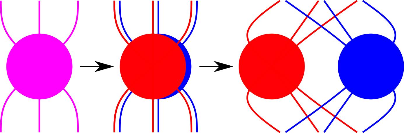
Two superalgebras are said to be (graded) Morita equivalent if their categories of graded modules are equivalent. When are simple, they each have a unique simple graded module (up to isomorphism, including parity change) [35], and so Morita equivalence means that the superalgebras of module endomorphisms (the “commutants”) of these modules are isomorphic. This relation between simple superalgebras is known as Brauer-Wall equivalence [36, 35]; another formulation, more useful for our purposes, says that are equivalent if they are related by stacking with matrix algebras; that is, if for some [37]. It is easy to see that the operation of stacking is compatible with this equivalence, so that one may speak of stacking equivalence classes: . It is worth emphasizing that the state sum construction takes as input a real superalgebra; forgetting the graded structure identifies many of these (and their Morita classes), as does complexifying and forgetting the real structure.
It will be shown in section IV.E that the pin TQFT corresponding to the algebras , with , is the unit in the monoid of pin TQFTs under stacking; in particular, it has state spaces and partition function for any closed pin surface . This fact justifies the conclusion that Morita equivalent algebras define the same TQFT, , up to an Euler term.
The Morita-invariance of the state sum construction motivates us to focus on certain convenient representatives from each Morita class. There are ten Morita classes of simple real superalgebras [36]. Eight of them are central simple and form a group under stacking. The real Clifford superalgebra — discussed in section IV.B — lives in the class labeled by its signature [13]. The remaining two Morita classes are non-central and do not have inverses under stacking. They are represented by the complex Clifford superalgebras , with being Morita invariant. In light of the result of section IV.C that the theory has partition function ABK, our discussion of stacking and Morita equivalence means that the algebra has partition function .
IV.E Invertible pin TQFTs
An invertible pin TQFT is one whose state spaces are one dimensional and whose partition functions on closed pin spacetimes are nonzero. Unitary2121 21 The assumption of unitarity is crucial. The non-unitary theory built from with has the same cobordism-invariant partition functions as the unitary theory built from with ; the two theories are distinguished on the macaroni cobordism. invertible theories2222 22 To be precise, we mean unitary invertible theories with values in supervector spaces. have a special property [40, 41]: not only are they completely determined by their partition functions on closed pin manifolds, these partition functions must be a cobordism invariant — a power of the ABK invariant — times an Euler term for .2323 23 Invertible pin TQFTs do not generate a complete set of pin diffeomorphism invariants, as the bounding torus and bounding Klein bottle cannot be distinguished: they have both ABK and trivial. In particular, if , the partition functions are cobordism-invariant and multiplicative under the appropriate notion of connect sum. These theories have been constructed as extended TQFTs in ref. [9]. Since and , the partition function on (alternatively, ) determines and therefore the full pin TQFT. In the following, we will compute the partition functions of for the theories associated to the real superalgebras and and find that they are and , respectively, up to Euler terms. Since these theories are invertible and unitary, this demonstrates that the state sum for matrix algebras is trivial — as claimed in section IV.D — while that for is the theory — in agreement with the findings of section IV.C.
A ribbon diagram for is depicted in Figure 11. It evaluates to
| (35) |
The matrix algebra is spanned by a basis of matrices with . The trace form is
| (36) |
Let be if and otherwise. The grading on is given by . acts trivially in this basis, and has a Hermitian structure given by conjugate transposition: . Therefore, by the discussion in section IV.A, the half twist is . Then compute
| (37) |
as claimed. Meanwhile was discussed in section IV.B. Let . Then compute
| (38) | ||||
This completes our argument. As a consistency check, one may evaluate the state sums on other closed pin manifolds and verify that they yield powers of the ABK invariant. This was done in ref. [7] for orientable pin (spin) surfaces. They show that yields partition function .
Acknowledgments
The author is especially grateful to John Barrett for acquainting me with the key references [7, 15], for productive discussions in the early stages of this project, and for sharing his thoughts on the manuscript. I would also like to thank Dave Aasen, Matt Heydeman, Nick Hunter-Jones, Anton Kapustin, and Eric Samperton for enlightening conversations and Arun Debray for valuable commentary on the manuscript. This work was performed partly at Fudan University and was supported in part by the U.S. Department of Energy, Office of Science, Office of High Energy Physics, under Award Number de-sc0011632 as well as the Simons Investigator Award.

References
- [1] L. H. Kauffman, “State models and the Jones polynomial,” Topology, 26(3), 395-407 (1987).
- [2] K. Shiozaki, S. Ryu, “Matrix Product States and Equivariant Topological Field Theories for Bosonic Symmetry-Protected Topological Phases in 1+1 Dimensions,” arXiv: 1607.06504
- [3] K. Shiozaki, H. Shapourian, K. Gomi, S. Ryu, “Many-Body Topological Invariants for Fermionic Short-Range Entangled Topological Phases Protected by Antiunitary Symmetries,” arXiv: 1710.01886.
- [4] A. Kapustin, A. Turzillo, M. You, “TQFT and MPS,” Phys. Rev. B 96, 075125 (2017).
- [5] A. Kapustin, A. Turzillo, M. You, “Spin TQFT and Fermionic MPS,” Phys. Rev. B 98, 125101 (2018).
- [6] L. Fidkowski, A. Kitaev, “Topological Phases of Fermions in One Dimension,” Phys. Rev. B, 83, 075103 (2011).
- [7] J. Barrett, S. Tavares, “Two-Dimensional State Sum Models and Spin Structures,” Commun. Math. Phys. 336, 63-100 (2015).
- [8] S. Novak, I. Runkel, “State Sum Construction of Two-Dimensional TQFTs on Spin Surfaces,” J. Knot Theory Ramifications 24 no.05, 1550028 (2015).
- [9] A. Debray, S. Gunningham, “The Arf-Brown TQFT of Surfaces,” arXiv: 1803.11183.
- [10] A. Turzillo, M. You, “Fermionic MPS and 1D SRE Phases with Anti-Unitary Symmetries,” Phys. Rev. B 99, 035103 (2019).
- [11] N. Bultinck, D. J. Williamson, J. Haegeman, F. Verstraete, “Fermionic matrix product states and one-dimensional topological phases,” Phys. Rev. B95,075108 (2017).
- [12] A. Lauda, H. Pfeiffer, “State sum construction of two-dimensional open-closed Topological Quantum Field Theories,” arXiv: math/0602047
- [13] M. Atiyah, R. Bott, A. Shapiro, “Clifford Modules,” Topology, 3 (Suppl. 1): 3–38 (1964).
- [14] R. C. Kirby, L. R. Taylor, “Pin structures on low dimensional manifolds,” Geometry of low-dimensional manifolds, 2, 177-242 (1989).
- [15] U. Pinkall, “Regular Homotopy Classes of Immersed Surfaces,” Topology Vol. 24. No. 4, 421-434 (1985).
- [16] I. James, E. Tomas, “Note on the classification of cross-sections,” Topology. 4 351-359 (1966).
- [17] K. Schlichting, “Regultire Homotopie geschlossener Flachen,” Diplomarbeit TU Berlin (1977).
- [18] W. H. Meeks III, J. Patrusky, “Representing homology classes by embedded circles on a compact surface,” Ill. J. Math. 22 262-269 (1978).
- [19] E.H. Brown, “Generalizations of the Kervaire invariant,” Ann. Math. 95 368-383 (1972).
- [20] G. Segal, “The Definition of a Conformal Field Theory,” in Topology, Geometry and Quantum Field Theory, ed. U. Tillmann, London Math. Soc. Lect. Note Ser., Vol. 30 8, p.421-577 (2004).
- [21] G. W. Moore, G. Segal, “D-branes and K-theory in 2D topological field theory,” arXiv: hep-th/0609042.
- [22] V. Turaev, P. Turner, “Unoriented topological quantum field theory and link homology,” Algebraic & Geometric Topology 6, 1069 (2006).
- [23] S. Fukuma, A. Hosono, H. Kawai, “Lattice Topological Field Theory in two dimensions,” Comm. Math. Phys. 161, no. 1, 157-175 (1994).
- [24] L. H. Kauffman, “An invariant of regular isotopy,” Trans. Am. Math. Soc. 318, 417-471 (1990).
- [25] P. J. Freyd, D. N. Yetter, “Braided compact closed categories with applications to low-dimensional topology,” Adv. Math., 77(2) 156-182 (1989).
- [26] D. N. Yetter. “Category theoretic representations of knotted graphs in s3,” Adv. Math., 77(2) 137-155 (1989).
- [27] L. H. Kauffman. “Knot diagrammatics,” Handbook of Knot Theory, 233-318, Elsevier (2005).
- [28] N. Yu. Reshetikhin, V. G. Turaev, “Ribbon graphs and their invariants derived from quantum groups,” Comm. Math. Phys., 127(1) 1–26 (1990).
- [29] O. Viro, “Quantum Relatives of the Alexander Polynomial,” St. Petersburg Math. J., Vol. 18, No. 3, 391-457 (2007).
- [30] U. Pachner, “P.l. homeomorphic manifolds are equivalent by elementary shellings,” Eur. J. Comb., 12(2) 129-145 (1991).
- [31] W. B. R. Lickorish, “Simplicial moves on complexes and manifolds,” In Proceedings of the Kirbyfest (Berkeley, CA, 1998), volume 2 of Geom. Topol. Monogr., 299-320 Geom. Topol. Publ., Coventry (1999).
- [32] A. Coward, M. Lackenby, “An upper bound on Reidemeister moves,” American Journal of Mathematics, 136 1023-1066 (2014).
- [33] V. Turaev, “Homotopy Quantum Field Theory,” EMS Tracts in Mathematics Vol. 10 (2010).
- [34] D. S. Freed, M. J. Hopkins, “Reflection positivity and invertible topological phases,” arXiv: 1604.06527.
- [35] P. Deligne, “Notes on Spinors,” Quantum Fields and Strings: a Course for Mathematicians, vol. 1, AMS. Providence, RI, pp. 99–135 (1999).
- [36] C. T. C. Wall, “Graded Brauer Groups,” Journal für die reine und angewandte Mathematik, 213, 187-199 (1964).
- [37] T.-Y. Lam, “Introduction to Quadratic Forms over Fields,” Graduate Studies in Mathematics Vol. 67, American Mathematical Soc. (2005).
- [38] C. Arf, “Untersuchungen über quadratische Formen in Körpern der Charakteristik 2, I,” J. Reine Angew. Math. 183, 148-167 (1941).
- [39] D. Johnson, “Spin structures and quadratic forms on surfaces,” J. London Math. Soc. (2) 22 no. 2, 365-373 (1980).
- [40] K. Yonekura, “On the cobordism classification of symmetry protected topological phases,” arXiv: 1803.10796.
- [41] D. S. Freed, G. W. Moore, “Setting the quantum integrand of M-theory,” Commun. Math. Phys. 263, 89-132 (2006).