A Physical Picture of Bispectrum Baryon Acoustic Oscillations in the Interferometric Basis2018A Physical Picture of Bispectrum Baryon Acoustic Oscillations in the Interferometric Basis–References
Abstract
We present a picture of the matter bispectrum in a novel “interferometric” basis designed to highlight interference of the baryon acoustic oscillations (BAO) in the power spectra composing it. Triangles where constructive interference amplifies BAO provide stronger cosmic distance constraints than triangles with destructive interference. We show that the amplitude of the BAO feature in the full cyclically summed bispectrum can be decomposed into simpler contributions from single terms or pairs of terms in the perturbation theory bispectrum, and that across large swathes of our parameter space the full BAO amplitude is described well by the amplitude of BAO in a single term. The dominant term is determined largely by the kernel of Eulerian standard perturbation theory. We present a simple physical picture of the BAO amplitude in each term; the BAO signal is strongest in triangle configurations where two wavenumbers differ by a multiple of the BAO fundamental wavelength.
Keywords:
dark energy – cosmological parameters – distance scale – cosmology: theory1 Introduction
The Baryon Acoustic Oscillation (BAO) method (Eisenstein et al. 1998; Blake & Glazebrook 2003; Hu & Haiman 2003; Linder 2003; Seo & Eisenstein 2003) has become a central means of pursuing the essential nature of dark energy, a mysterious substance making up roughly of the present-day Universe. The BAO method uses the imprint of sound waves in the early Universe on the late-time clustering of galaxies to probe the cosmic expansion history, which through general relativity is linked to dark energy.
The BAO method has been applied to the galaxy 2-point correlation function (2PCF) and power spectrum (Ross et al. 2017; Alam et al. 2017), as well as more recently to the galaxy 3-point correlation function (3PCF) (Gaztanaga et al. 2009; Slepian et al. 2017a; Slepian et al. 2017b) and bispectrum (Pearson & Samushia 2018), measuring respectively 2- and 3-point clustering over random in configuration space and Fourier space. While measurements of the bispectrum and 3PCF have improved BAO constraints over those of the power spectrum alone, optimal constraints are difficult to obtain given the large number of bispectrum triangles. Bispectrum covariance matrices are often estimated from mock catalogs (Gaztanaga et al. 2009; Pearson & Samushia 2018; though other approaches exist, see Slepian et al. 2017a; Slepian et al. 2017b). In order to properly estimate covariance matrices, the number of mock catalogs must greatly exceed the number of triangles (Percival et al. 2014); when many triangles are used to constrain BAO, the number of mocks needed is unrealistic with present computational resources. For example, Pearson & Samushia 2018 measured the bispectrum for a large number of triangles, but noted that their error bars were limited by the number of mocks available to estimate the covariance matrix; more mocks would improve their 1.1% precision joint constraints substantially to 0.7%, a gain of more than 30%.
With better understanding of which bispectrum triangles are most sensitive to BAO, future studies could obtain better BAO constraints with a smaller set of triangles and, therefore, a smaller covariance matrix. These triangles could be identified by measuring all bispectrum triangles and their covariances, but such an approach also faces the problem of limited mock catalogs. Because fully -body mocks cannot presently provide a good estimate of the full covariance matrix of all bispectrum triangles, we must select a set of optimal triangles for BAO constraints—without knowledge of the full covariance matrix.
Recently, our work in Child et al. 2018 proposed one technique to select bispectrum measurements that are sensitive to BAO. We highlighted that BAO in the bispectrum constructively interfere in certain triangle configurations, amplifying the BAO signal. In a short work, we measured bispectra only on triangles where the BAO signal is amplified. With this relatively small set of bispectrum measurements we found substantial improvements in BAO constraints over power spectrum measurements alone, equivalent to lengthening BOSS by roughly 30%. Our method for triangle selection greatly reduced the number of bispectrum measurements necessary to obtain such an improvement.
In detail, at leading order the bispectrum involves products of two power spectra; each power spectrum introduces an oscillatory BAO feature. When the oscillations are in phase, they amplify the BAO signal. In our earlier paper, we showed that this constructive interference increases the amplitude of BAO in the bispectrum. We introduced a new parametrization of bispectrum triangles: instead of the three triangle sides , , and , we use the length of one triangle side , the difference in length of the second from the first in units of the BAO fundamental wavelength, and the angle between them . We computed the BAO amplitude for a selection of triangle configurations, producing a map of the root-mean-square (RMS) amplitude as a function of the length difference and the opening angle. Using this RMS map, we can surgically identify the configurations most suitable for studies of BAO in the bispectrum.
The “interferometric basis” proposed in our earlier work promises other applications beyond improvement in BAO constraints with relatively few bispectrum measurements. First, since our method identifies the triangles that are most sensitive to BAO, it offers an approach to more efficiently investigate the independence of bispectrum information from that obtained via reconstruction (Eisenstein et al. 2007; Noh et al. 2009; Padmanabhan et al. 2009; Padmanabhan et al. 2012) and the covariance between the bispectrum and power spectrum. Second, our parameterization allows intuitive visualization of BAO in the bispectrum. Third, our interferometric approach is sensitive to phase shifts associated with (such as that driven by relativistic neutrinos at high redshift (Baumann et al. 2017)), spinning particles in the early Universe (Moradinezhad Dizgah et al. 2018), or relative velocities between baryons and dark matter (Dalal et al. 2010; Tseliakhovich & Hirata 2010; Yoo et al. 2011; Slepian et al. 2018).
In this paper, we investigate more fully the physics of BAO in the interferometric basis. The bispectrum is a sum of three cyclic terms, but for many triangles, the cyclic sum is dominated by only one or two of the three terms. Which term dominates is determined primarily by the kernel of Eulerian standard perturbation theory (SPT). Products of power spectra also enter the leading-order perturbation theory (PT) bispectrum, but their role in the dominance structure is secondary; instead, they introduce the oscillatory features whose interference is highlighted by our basis.
When the bispectrum is dominated by only one or two terms, the amplitude of BAO in the full bispectrum can be approximated by the BAO amplitude in the dominant term or terms. We show analytically that because BAO are a small feature in the power spectrum, the difference between the RMS amplitude computed under this approximation and the full RMS amplitude vanishes at leading order. We can therefore decompose the full RMS map into approximate “eigen-RMSes” computed from individual terms. Numerical work verifies that this decomposition successfully reproduces the primary features of the full RMS map.
To understand these features, we study the behavior of BAO in each term and pair of terms that can dominate the bispectrum. The structure of the power spectrum, in particular BAO and their envelope due to Silk damping, determines the RMS amplitude. For each triangle configuration, the BAO amplitude in each term is driven by one of four interactions between power spectra: interference, incoherence, feathering, or single power spectrum. The first, interference, can dramatically amplify BAO amplitude in certain configurations, like those used in Child et al. 2018 to constrain the BAO scale.
In general, then, the kernel determines which pairs of power spectra set the amplitude of BAO in the measured bispectrum. The remainder of the paper details this broad picture as follows. In §2, we review the interferometric basis as presented in our earlier work, and define the RMS amplitude of the ratio of physical to “no-wiggle” bispectrum we use in our analysis. §3 introduces notation used throughout. §4 shows which triangle configurations are dominated by a single term of the bispectrum cyclic sum; in these regions, the BAO signal in the bispectrum simplifies to the BAO signal in a single term, as shown analytically in §5. In §6, we numerically calculate the BAO amplitude in each term of the cyclic sum. These “eigen-RMSes” approximate the BAO amplitude in the full bispectrum in the regions where the corresponding terms dominate, and they assemble into a picture that matches the full map of BAO amplitude. §7 presents implications of our study for the reduced bispectrum, the 3PCF, and multipole expansions of the 3PCF and bispectrum. §8 concludes.
Throughout we adopt a spatially flat CDM cosmology at consistent with the WMAP-7 (Komatsu et al. 2011) parameters of the MockBOSS simulations (Sunayama et al. 2016) used in Child et al. 2018: , , , , and .
2 Interferometric Basis
Several sets of triangle parameters have been used in previous works for the isotropic bispectrum and three-point correlation function (3PCF). Sefusatti et al. 2010, Kayo et al. 2013, and Baldauf et al. 2015 considered the bispectrum for equilateral or isosceles triangles. Scoccimarro et al. 1998, Scoccimarro 2000, Bernardeau et al. 2002, Sefusatti et al. 2010, Baldauf et al. 2012, Gil-Marín et al. 2012, and Hikage et al. 2017 used one side , the ratio of a second side to the first , and the angle between the two ; the third side can also be parameterized simply as (Pearson & Samushia 2018) or by its ratio to (Jeong & Komatsu 2009; Baldauf et al. 2015). Scoccimarro 2000 and Sefusatti et al. 2006 allowed each triangle side to be any integer multiple of the bin width .
Like the bispectrum, the 3PCF can be parametrized using one side , the ratio of a second side to the first , and the opening angle (Kulkarni et al. 2007; Marín 2011; Marin et al. 2013). Other parameterizations use two sides and . The third parameter can be the opening angle between them (McBride et al. 2011a; McBride et al. 2011b; Guo et al. 2014; Guo et al. 2015), the cosine of the opening angle (Gaztanaga et al. 2009), a shape parameter combining the three side lengths (Peebles 1980; Jing & Börner 2004; Wang et al. 2004; Nichol et al. 2006), or a multipole expansion of the dependence on opening angle (Szapudi 2004; Pan & Szapudi 2005; Slepian et al. 2017a; Slepian et al. 2017b). Many studies of the anisotropic bispectrum and 3PCF, which retain information about the line of sight, have also employed a multipole basis with respect to the line of sight in redshift space (e.g. Gagrani & Samushia 2017; Yamamoto et al. 2017; Castorina & White 2018; Desjacques et al. 2018; Nan et al. 2018; Yankelevich & Porciani 2018). Slepian & Eisenstein 2018 and Sugiyama et al. 2018 use a spherical harmonic expansion of the 3PCF and bispectrum, which includes information on both the internal angle and the angles to the line of sight.
In Child et al. 2018, we introduced a new basis for bispectrum work motivated by the physics of BAO in the bispectrum. The bispectrum involves products of linear matter power spectra (e.g. Scoccimarro et al. 1998), as
| (1) |
We refer to as the pre-cyclic term, and to the terms denoted by cyc. as the post-cyclic terms. is the Eulerian standard perturbation theory kernel that generates a second-order density field when integrated against two linear density fields. The kernel depends only on two side lengths and and the angle between them (through the dot product ):
| (2) |
We will refer to the middle term of equation (2), , as the dipole contribution to .

The power spectra in equation (1) have BAO features that oscillate sinusoidally. These features can thus interfere, motivating us to consider a parameterization of the bispectrum that transparently captures the phase structure. In particular, we set up our parametrization to capture the phase structure of the pre-cyclic term (first term in equation 1) in and , as follows:
| (3) |
Throughout this work we assume without loss of generality that is positive, so . The external angle is shown in Figure 1. The fundamental wavelength of the BAO in Fourier space is given by
| (4) |
where is the effective sound horizon evaluated at a fiducial wavenumber . As discussed in Eisenstein & Hu 1998, the lowest-wavenumber nodes of the baryonic transfer function occur at higher wavenumber than the nodes of . The effective sound horizon grows with for and asymptotes to the sound horizon for ; we define according to its asymptotic value at .
We use “configuration” to describe a set of triangles with fixed and over the range . For each configuration, we divide into 100 bins of width . The other two wavenumbers and are calculated from each according to equation (3). We study configurations with and , with 80 points in and 80 in for a total of 6400 configurations. We sample many points simply to produce well-resolved figures, but we note that configurations that are close to each other in space are highly covariant.
We restrict to the range and to be less than about 4 to capture most of the effects of BAO. For most configurations, is smaller than the other two triangle sides, but for small and , can be smaller than . In our previous paper, these configurations were not used to constrain BAO because they are subject to cosmic variance and covariant with the power spectrum (as discussed under “Simulations” in Child et al. 2018).
Below our minimum wavenumber of , cosmic variance becomes significant; given the mock catalogs we use one cannot make a sufficient number of subdivisions to estimate covariances on these large scales. Of course at large scales the covariance should be dominated by the Gaussian Random Field (GRF) contribution, so a template could be used to model the covariance (e.g., as Slepian & Eisenstein 2015 does for the isotropic 3PCF and Slepian & Eisenstein 2018 for the anisotropic 3PCF).
However, even with an adequate covariance, the contribution of low-wavenumber modes to BAO constraints should be small given the small number of large-scale modes in the volume of a survey such as DESI11 1 http://desi.lbl.gov (DESI Collaboration et al. 2016). Our minimum wavenumber corresponds to a physical scale of ; DESI will have volume of order equivalent to a box side length of roughly . Thus there are of order 200 modes of wavelength in the box, enabling measurement to about 7% precision. The contribution of low-wavenumber bispectrum modes to BAO constraints will therefore be negligible compared to the 0.1% precision DESI will achieve using power spectrum BAO at higher wavenumber. It is the case that the other two triangle sides can probe higher wavenumbers—our maximum studied is , so corresponds to at most and . These wavenumbers do access BAO scales, but nonetheless, the bispectrum error bar will not be competitive with DESI power spectrum precision as the total bispectrum error bars of such configurations will be dominated by the cosmic variance of the shortest side .
At higher wavenumbers than our maximum, even at the level of linear theory Silk damping (Silk 1968) degrades the BAO signal. The Silk damping scale (equation 7 of Eisenstein & Hu 1998), is approximately for our cosmology; at wavenumbers above , the BAO signal in the transfer function is increasingly suppressed as (equation 21 of Eisenstein & Hu 1998).
Wavenumbers above are nonlinear, so perturbation theory no longer provides an accurate model of the bispectrum at these scales (Rampf & Wong 2012). Effective field theory (EFT) models perform reasonably well up to ; Carrasco et al. 2012 describes the power spectrum to the percent level for . In the case of the bispectrum (e.g. Bertolini & Solon 2016; Nadler et al. 2018; de Belsunce & Senatore 2018), the maximum wavenumber at which EFT agrees with simulations depends on configuration and cosmology, but EFT models of the real-space matter bispectrum perform well up to (Angulo et al. 2015; Baldauf et al. 2015). In redshift space, however, perturbation theory models break down at yet smaller wavenumbers, differing from bispectrum measurements at the 10% level by (Smith et al. 2008).
Baryonic effects, which are not as yet satisfactorily modeled, also become important at wavenumbers above our maximum. For , hydrodynamical simulations find a alteration in the power spectrum relative to dark-matter-only simulations (Chisari et al. 2018). As the bispectrum scales roughly as with the power spectrum, this uncertainty in the power spectrum likely translates to in the bispectum, which at tree level is proportional to the square of the power spectrum (see also the hierarchical ansatz of Groth & Peebles 1977). In the absence of a theoretical model for baryonic effects, the uncertainty in high-wavenumber models of the bispectrum is much too large to measure BAO to sub-percent precision.
Overall, then, the range of wavenumbers we consider is a conservative cut to isolate the regime where BAO effects are most prominent and the bispectrum is best understood. Within this range of scales, our interferometric basis identifies the configurations where constructive interference of power spectra amplifies the BAO “wiggles.” To quantify the presence of BAO in each configuration, we compute the RMS amplitude of the ratio of the bispectrum to its no-wiggle analog . We have
| (5) |
where the numerator is computed using power spectra from CAMB (Lewis et al. 2000) and the denominator using power spectra from the fitting formula for the no-wiggle transfer function of Eisenstein & Hu 1998. The variance is
| (6) |
where is the mean of on the same range, . Figure 2 shows the root-mean-square amplitude for a selection of configurations. Throughout this work we will refer to Figure 2 as the root-mean-square (RMS) map.

Our basis is a transformation of the triangle sides ; the axes and of our RMS map correspond roughly to and , respectively. In our basis, the wavenumbers and depend on , , and as
| (7) |
where the first equality for stems from the orientation of shown in Figure 1 and the law of cosines. Configurations with the same therefore lie along sloped curves in the plane. As the power spectrum depends only on the magnitude of the wavenumber, these curves are also traces of constant .
The parameter was chosen to produce constructive interference in the precyclic term of the bispectrum (first term in equation 1). However, constructive interference is not limited only to this single term: we expect interference as well where and , or and , differ by integer multiples of the BAO wavelength . We calculate the configurations for which these conditions are satisfied. Curves where are horizontal lines in the plane, as shown in the left panel of Figure 3; that is, where
| (8) |
The curves where , shown for in Figure 3, are given by
| (9) |
We only show the case as higher harmonics of do not correspond to features in the RMS map, as discussed in §6.1.2 below. The curves where , shown as dashed curves in the right panel of Figure 3, follow
| (10) |

In general, equations (9) and (10) depend on both and . In the special case of the equilateral configuration, the dependence cancels; that is, when and , equation (9) gives . For these configurations, equals for all . For all other configurations, however, equations (9) and (10) can only be satisfied for a single . When necessary, we choose a representative value of to compute the configurations for which equations (9) and (10) hold.
3 Notation
Here we define notation for several combinations of power spectra, kernels, and bispectra that will be used throughout.
BAO in the bispectrum come only from oscillations in the power spectrum, which we isolate as
| (11) |
where is defined through this equality and represents the BAO-only piece of the power spectrum. We note that ; the baryon fraction in our Universe is small (), so the BAO are a small feature in the power spectrum.
Each term in the cyclic sum (1) is denoted by
| (12) |
with
| (13) |
and
| (14) |
The ratio of each term to its no-wiggle analog is
| (15) |
where the second equality holds because the kernel is unaltered going from a physical to a “no-wiggle” cosmological model. The kernel stems from the Newtonian gravity solution of the equations of perturbation theory assuming an Einstein-De Sitter (matter-dominated) cosmology, and is thus independent of the input linear power spectrum. We note that all cosmological parameters of the no-wiggle model, including the matter density, are identical to the physical model.
Using the definition (11) of , we may rewrite
| (16) |
where the last equality defines , the oscillatory piece of one term of the bispectrum (1).
To refer to a ratio where one term in the sum is negligible, we use
| (17) |
The sum is not equal to of equation (5).
4 Regions of Dominance
In order to understand the behavior of the BAO amplitude shown in the RMS map (Figure 2), we seek to identify configurations where the cyclic sum of the perturbation theory bispectrum (1) simplifies. That is, we ask whether there are any regions where the behavior of the full bispectrum is determined by only one or two of the three terms in the cyclic sum.

Figure 4, our “dominance map,” shows that many of the configurations are indeed dominated by a single term (red and blue regions), and others are dominated by two terms while the third is negligible (green and purple regions). The RMS map (Figure 2) reflects the dominance structure. The horizontal bands at (red region, dominant) transition to sloped bands in the purple and black regions. The blue region ( dominant) corresponds to a pattern of small maxima and minima in the RMS map that we call “feathering.” Finally, in the green region at low and high , RMS amplitude is maximized for triangles where two wavevectors are nearly antiparallel and the third is small. The mechanisms that drive these different patterns in each region are described in detail in §6 below.
In this section, we detail the calculation and behavior of the dominance map (Figure 4). In §4.1, we present our definitions of dominance, which require the choice of a factor . The specific ways in which triangle geometry determines which term dominates are discussed in detail in §4.3; the dominance map is driven primarily by the behavior of the kernel reinforced by the broadband behavior of the power spectrum, as we will further detail in §4.2. In most regions of the dominance map, the maximum and minimum terms in the kernel also maximize or minimize the power spectrum; the exceptions are discussed in §4.4. In general, in the squeezed limit where one side of the triangle can be much larger than the smallest, terms including the largest wavenumber are small. In the other limit, an equilateral triangle, all three sides are similar so all functions of them are similar as well and no sides dominate. The dominance plot shows the transitions between these two regimes.
We note that we assume positive , and for , no region is dominated by (yellow) or the pair of terms (orange). When , and interchange. This would correspond to mirroring across the -axis; blue would become yellow.
4.1 Definition of “Dominance” and Choice of Dominance Ratio
We identify dominant terms by comparing the magnitudes of terms across . The dominance structure is determined by the broadband behavior of the bispectrum terms, so we use the no-wiggle bispectrum to fully isolate the broadband. Results are similar when the full bispectrum is used instead, as BAO are small relative to the broadband.
At each (, ) configuration, we calculate the ratios between each pair of terms as a function of . We then compare the medians, denoted , of these ratios to a factor . We use the median because it is a smooth function of our parameters and , unlike the mean, which can be skewed by large ratios between the terms at small . The median is more representative of the typical ratio across all we consider.
Dominance criterion—If exceeds each other term by at least a factor of , that is, if
| (18) |
we consider dominant.
Double dominance criterion—If two of the terms that enter the bispectrum determine its behavior while the third is relatively small, we say that two terms are double dominant. Two ratios must be within a factor of of each other but both exceed the third by at least a factor of . Because terms can be either positive or negative, this comparison alone is not obviously sufficient; one term could be large and positive, and the other large and negative, such that their sum is smaller than the third term. Therefore we also require the sum of the two dominant terms to exceed the third term by a factor . Our double dominance criterion is thus a set of four conditions: and are both dominant and only is negligible when
| (19) |
In practice, the final condition is not relevant for any configuration we test; the differences between large positive and negative terms remain much larger than the third term, for example in the region described in further detail in §4.3.4.
No term dominant—If the medians of all three ratios are within of each other, then no term is dominant.

The dominance region plot is weakly dependent on the choice of the factor , as shown in Figure 5. As the threshold for dominance rises, less of the plane is dominated by a single term; the -dominant, -dominant, and no-term-dominant regions encroach on the single-term-dominant regions. We choose as our standard threshold for dominance, as it is sufficiently large to separate the term that dominates the RMS amplitude. With this choice of , the non-dominant terms are typically less than 20% of the dominant term, so the ratio of the bispectrum to the no-wiggle bispectrum (5) can be Taylor-expanded about the ratio of a single term in the cyclic sum to its no-wiggle analog (as we do in §5).
4.2 Kernel Drives Dominance Structure
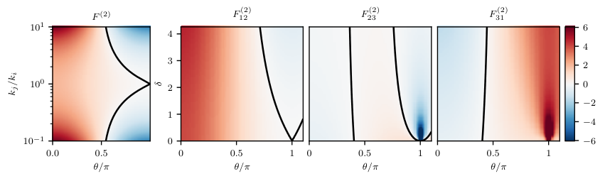
As seen in Figure 6, the structure of the full dominance plot strongly resembles that of a dominance plot for alone, which itself reflects the behavior of in the - plane (Figure 7).
Including expands some regions (near their borders, can move the maximum term from just under to just over the next-largest term). In Figure 6, we choose for the and panels to agree with our choice of for the product . As discussed in §4.3 (equation 20), the and dominance criteria cannot simply be multiplied together to determine dominance in , but these two contributions independently illuminate the full bispectrum dominance map.

The dynamic range of is larger than that of , so the kernel determines most of the dominance map of Figure 4. The middle term of the kernel, in equation (2), varies the most between configurations: it can be positive or negative, and can be very large when one side is much smaller than the other (for example, surrounding in Figure 7). Alternatively, can approach arbitrarily close to zero (black curves in Figure 7).
4.3 Regions of the Dominance Map
In this section, we step through each region of the dominance plot of Figure 4 from left to right to discuss the dominance behavior. In general, the relative magnitudes of the , , and differ across configurations due to differences in the dependence of the three wavenumbers , and (given in equation (7) and Figure 3).
For each region, we discuss the behavior of the and that enter the bispectrum. We build up understanding of each region by first analyzing their behavior separately, then considering the implications for the full dominance plot. We take this approach because the power spectrum products behave very differently from the kernels, even though dominance is determined by the median ratios of terms , which are medians of products and not products of medians:
| (20) |
We note that the power spectrum is maximal at ; above , declines monotonically as . Since our analysis covers the range , it is a good approximation that in our -range of interest the broadband power spectrum falls as . This approximation fails only in the low-, high- region where can be sufficiently small that increases with (discussed in §4.3.4 below).
4.3.1 Red region, dominant
When , Figure 4 shows that is the dominant term in the bispectrum cyclic sum (1). In this red region, configurations are constructive where and (defined in equation 11) are in phase, and destructive where they are out of phase. dominates because in both the kernel and the products of power spectra , the pre-cyclic terms are largest.
is much larger than and (as shown in Figure 7) because only in is the sign of the dipole contribution positive. The dot product of the unit vectors and , which determines the sign of the dipole contribution, approaches in . For and , the relevant dot product instead approaches . While and therefore contain both positive and negative contributions of similar magnitude, all contributions to are positive, so will be the largest . For example, where vanishes as well as (in the lower left corner, symbol), two sides, and , are equal, while . With these side lengths and dot products, and . exceeds the other two by a factor of eight.
The effect of the power spectrum products is to further separate the three cyclic terms. For , the triangle is obtuse (see in Figure 1). As and the triangle fully opens, approaches . For these obtuse triangles (see Figure 3) because always exceeds . The power spectrum is monotonically decreasing, so the ordering implies . Thus , reinforcing the order of the .
For nonzero (e.g., symbol in Figure 4), grows with , but remains dominant by our dominance criterion of . For large , is small relative to . The other two wavenumbers and are both larger than (Figure 3), so approaches . As a result, and are of similar magnitude (as in the purple region at low and high in the leftmost panel of Figure 6). The magnitudes of the and kernels also grow as increases, with the kernel approaching but remaining smaller than . As continues to increase, comes within a factor of 10 of , causing a purple region to appear in the upper left corner of the right panel of Figure 5. We note that this effect is too small to appear when the dominance criterion is , our choice in the main analysis of this work (as in Figure 4).
4.3.2 Middle region, no term dominant (black) or and dominant (purple)
Around , at most one term in the cyclic sum can be neglected. In the black region at low , all three terms are of comparable magnitude; in the purple region at larger , shrinks, but and are still large and of similar magnitude. The black region contains triangles that are nearly equilateral; triangles with and are equilateral for all . Since all three sides and angles are equal, all three terms in the bispectrum are identical, and no term can dominate any other.
In the purple region, is negligible compared to and . As increases along the line shown in Figures 3 and 4, and grow larger than . Since , and remain equal; their ratio will deviate little from unity. But as increases, both and shrink relative to the other terms. In particular, approaches zero. For large along , the unit vectors and are antiparallel as is relatively small, and their dot product becomes . Since , the dipole contribution in the kernel, and therefore vanishes. Furthermore, Figure 3 shows that at large , and are much larger than . The product of power spectra is therefore smaller than the other two products and , which both involve the much larger . Both and shrink as increases, so becomes smaller than the other two terms and can be neglected. Thus and dominate the bispectrum cyclic sum.
4.3.3 Blue region, dominant
At the right side of Figure 4, where is large (circle symbol), dominates the cyclic sum. Both and are large relative to the other kernels and products of power spectra.
In the kernel, as shown in Figure 7, vanishes, and negative contributions to make it smaller than . vanishes because in this region, triangles are in the squeezed limit, where . The third wavenumber approaches , meaning
| (21) |
so is small relative to the other two wavenumbers (see Figure 3). At the same time, the dot product approaches , so behaves as
| (22) |
In equation (22), the difference between and (3) is much smaller than , so and vanishes. Meanwhile, the other two terms do not vanish; but , so and approach
| (23) |
| (24) |
The magnitudes of and are comparable, so the dipole contributions in (equation 23) and in (equation 24) are similar in magnitude. Only in do both contributions have the same sign, so is larger than .
The reinforce the behavior of the kernel. is small, but still large enough that is monotonically decreasing; for of a few, equation (21) is near (§4.3). In this limit , so must be the largest of the three wavenumbers. In the power spectrum, then, . and , which include , are therefore smaller than , which does not. The largest power spectrum term is therefore as in the kernel, and dominates the bispectrum.
4.3.4 Green region, and dominant
In the lower right corner of Figure 4 around , (star symbol), the dominant terms are and . Dominance is once again driven by the kernel; and are very large (as shown in Figure 7) while vanishes.
vanishes for the same reason it does in the blue region, but the magnitude of is more comparable to that of than it is at higher . Along the line where , the blue region transitions to green at roughly (square symbol in Figure 4). Here, , which is nearing the lowest in our range (). Both and therefore exceed by up to a factor of . As in the blue region, triangles in the green region are squeezed, so the dot products between unit wavevectors are the same as in the blue region. The kernels then behave as equations (22–24), and (equation 22) vanishes. Unlike in the blue region, however, the dipole contribution is large enough that the constants in equations (23) and (24) become insignificant. and are thus both comparably large; is large and positive () while is large and negative (). This region satisfies our double dominance criterion (19), as even the sum exceeds the very small third term —for example, by a factor of at .
Our assumption that falls monotonically with breaks down in the green region. Because is proportional to (as in equation 21), becomes very small for small (see Figure 3). Our previous analysis assumed all wavenumbers were large enough that the power spectrum is monotonically decreasing, but in the green region, can be in the regime where increases with . Both and are still greater than , in the regime where falls with . For very small , then, may be smaller than and . As a result, can be the largest product of power spectra, despite the fact that and are much larger than . However, the power spectrum is overshadowed by the behavior of the kernel. Even for , where can exceed the other two products of power spectra by a factor of 25 at small , the median ratio of power spectra products, , is only 5. But the median ratio of kernels, , is of order because so nearly equals , driving to vanish. The dominance structure is thus driven primarily by the kernel.
4.4 Ordering of Subdominant Terms
The of equation (1) with maximum median is everywhere also the term with maximum median . The ordering of terms differs only in the regions shown in Figure 8, where the two subdominant terms are swapped. These regions arise because the kernel can be either positive or negative. In the range of wavenumbers of interest, the power spectrum is always positive but monotonically decreasing, so the products change smoothly. and , smaller than for small (see the left panel of Figure 6 and the top panel of Figure 9), cross above around the equilateral configuration (). is the first to cross above because , so . lags behind (see the top panel of Figure 9).

The behavior of the kernel (equation 2) is not as simple, as shown in the lower panel of Figure 9. First, it can be either positive or negative (see Figure 7), explaining the region in Figure 8 where the ordering of the subdominant terms differs between and . The difference arises because the absolute values of the two subdominant terms and spuriously cross when both are small. In detail, we take the absolute value of each , since the magnitudes of each term, not their signs, determine dominance. For , both and are negative, with more negative than . For , both terms are positive, with more positive than . must therefore cross above , and it does so in the same region around where both terms cross zero—but the terms are not equal to zero where they cross each other. As shown in Figure 7, the value of at which crosses zero depends on the ratio between the two sides and , so becomes positive at slightly lower than does . As approaches zero, its absolute value falls below the small and positive at (with , for example, as in Figure 9). After becomes positive, it crosses at . Meanwhile in the product of power spectra, the median exceeds the median for all . Therefore, in this narrow region where the median falls below the median , the smallest term is not the smallest term.
The order of the subdominant terms also differs around (Figure 8). Figure 9 shows that this region arises due to differences in the behavior of the median between the power spectrum and the kernel. The power spectrum decreases monotonically, so the median occurs at the median . Therefore and are equal when is evaluated at the median (see equation 10). In Figure 9, crosses above at (with ). Unlike the power spectrum, the kernel can be positive or negative, and in some configurations it is positive for some values of and negative for others. For these configurations, the absolute value of is not a monotonic function of , so its median does not necessarily occur at the median . Therefore crosses above at such that the that corresponds to the median equals the that corresponds to the median . In the example of Figure 9, the solution is . becomes the minimum at while does not become the minimum until . Therefore in the shaded region of Figure 9 between these two crossings (), the order of the subdominant terms differs.
In contrast, around , both and are positive for all . Their medians are both found at the median value of , so crosses above where (equation 9, evaluated at the median ). As the median occurs at the median , also crosses above where equation (9) is evaluated at the median . therefore becomes the maximum at the same value of where becomes the maximum .
Though we set out to explain the regions where the minimum differs from the minimum , our analysis also explains why the largest is always also the largest (see Figure 8). The median behaves most simply for and , which are both the maximum term at low . As increases, is always the first to cross , and is always the first to cross . and are never the maximum term because . The complexity of the ordering of subdominant terms arises from the and terms, but because these terms are never the maximum terms, the maximum term never differs between and .
5 Decomposition into Eigen-Root-Mean-Square Plots
We now show how the RMS amplitude (equation 6) can frequently be approximated as a linear combination of three terms. We first require an expression for the ratio (equation 5) of the full bispectrum (1) to its no-wiggle analog. We wish to leverage the fact that the BAO are a small fractional feature in the power spectrum, so we write
| (25) |
with the product of two no-wiggle power spectra and the BAO feature in the product (13) of linear power spectra. In particular we split the matter transfer function into smooth and oscillatory pieces as
| (26) |
where and are smooth functions of (Eisenstein & Hu 1998), is small (because ), and is the order zero spherical Bessel function.
The power spectrum is proportional to the primordial power spectrum and the matter transfer function as
| (27) |
We suppress the redshift dependence of the power spectrum for simplicity, as it does not affect our analysis. The products of power spectra are then
| (28) |
Taylor-expanding the fractions to leading order in we have
| (29) |
where we used the fact that the no-wiggle power spectrum is simply .
In the remainder of this section, we show that in regions where only one or two terms dominate the bispectrum, the variance of the full bispectrum is approximated to leading order by the variance of only the dominant term or terms. We first consider the case where one term is dominant and the other two negligible, and we then consider the case where one term is negligible and the other two must be retained.
5.1 Single Term Dominant
We first consider the case where one term in the bispectrum dominates over the other two; without loss of generality we take this to be the first term.
We calculate the RMS amplitude (equation 6) from the variance of the ratio , defined in equation (5) as
| (30) |
Our goal is to show that the variance of the approximate ratio
| (31) |
is the same as that of the full ratio, , to leading order in one or the other of two small parameters we define,
| (32) |
We first notice that the variance of is
| (33) |
the constant term in equation (31) of course contributes no variance. Since is second-order in the small parameter , we neglect all corrections at third order and higher. We will find that the difference between the full variance and the variance of vanishes at second order.
Factoring out the dominant term in the numerator and denominator of equation (31) and using the definitions above, we have the ratio as
| (34) |
In the second, approximate equality, we have Taylor-expanded the denominator to second order in . We include the second-order term for the moment but see that it drops out of our end result.
We now seek to exploit the fact that the BAO feature itself is small, i.e. (equation 29 with small ). Using as defined in equation (16) to simplify differences of and , we have
| (35) |
where to obtain the first equality we substituted the definitions (32) and to obtain the second we Taylor-expanded to leading order in . In the third equality, we defined
| (36) |
which is . The analog of equation (35) holds for the term by switching to everywhere.
We know the variance at leading order is from equation (33), so we only retain terms that are second order in a combination of and . Our approximate expression for the ratio is now
| (37) |
The first term is , the second and third , and the fourth and fifth . These last two terms cancel each other to second order; (equation 35) is itself second order, so at leading order the second to last term is equal to the last. Equation (38) then simplifies:
| (38) |
Now computing the expectation value of and factoring out to enable further Taylor expansions, we find
| (39) |
We now square the form above and multiply out to find
| (40) |
Now using equation (38) to compute the expectation value of , we obtain
| (41) |
The variance of is then
| (42) | ||||
Recalling that (equation 31) and denoting the variance of as , we find
| (43) | ||||
To second order, the difference (43) cancels. Thus, the difference between and is suppressed by one order relative to . Therefore is the leading contribution to the variance . When a single term dominates the bispectrum cyclic sum, the variance of that single term is a good approximation of the variance of the full bispectrum. In §6, we use this fact to better understand the behavior of the RMS map (Figure 2) in regions dominated by a single term.
5.2 Double Dominance
Our goal is to show that if the sum of two terms dominates the third in , then the variance of , , is well approximated by that of the two dominant terms, and that the error in making this approximation is one order higher than the result itself. The requirement that the sum of two terms is much larger than the remaining term is only one condition of our double dominance criterion (19), but this condition is sufficient to show that is well approximated by the contribution of only two terms. Our double dominance criterion is more strict in order to distinguish regions where two terms are both large from those where one term nearly dominates the full bispectrum, and its sum with either of the other two (comparably small) terms is much larger than the remaining term.
Without loss of generality we take . We again begin from equation (30) and calculate in terms of the variance of the two dominant terms, . We have
| (44) | ||||
where to obtain the second line we Taylor-expanded the denominator to second order in . We defined and its no-wiggle analog as
| (45) |
We also defined as the first factor in the first line of equation (44), as in equation (17). Multiplying out equation (44) and dropping terms, we obtain
| (46) |
The two small parameters and differ only in the BAO feature, which we again parameterize by (equation 16):
| (47) |
motivating us to define
| (48) |
where in the second, identical equality we are simply noting that we will drop the subscripts on . Physically, is the weighted average of the BAO features in the and terms in the bispectrum (1). Expanding equation (47) to second order in and , we find
| (49) |
So we see that
| (50) |
Retaining only terms at second order and lower, we then have
| (51) |
Now we have that to second order , and we find that
| (52) |
including all terms at second order and below.
Thus to second order the variance in the dominant terms differs from the variance in the full bispectrum only by
| (53) |
As in §5.1 above, the leading contribution to the difference has , in which case the two terms on the right side of equation (53) cancel. The error is therefore , where our notation indicates that the error is third order in small quantities but can have any combination of and reaching that order. In contrast, the result is second-order in . Thus we have shown that the error of approximating the variance of the full ratio by that of the ratio of the first two terms, , is one order smaller than the variance itself.
6 Numerical Eigen-Root-Mean-Square Calculations
As shown analytically in §5, in the regions of single and double dominance identified in §4, the RMS amplitude of BAO in the full bispectrum simplifies to the RMS amplitude of BAO in the dominant term or terms of the bispectrum cyclic sum (1). We calculate RMS maps for each single term and pair of terms . In Figure 10, we combine the single- and double-term RMS maps in the corresponding single- and double-dominance regions; the result matches the full RMS map of Figure 2 reasonably well. The simplified maps of therefore provide a good approximation to the full RMS map. In the remainder of this section, we fully detail the RMS maps for each single term (§6.1) and pair of terms (§6.2) over the full plane.

6.1 Single Term Dominant
While the BAO amplitude in the full bispectrum (1) is a complicated function of triangle configuration, many configurations have only a single term dominant, as discussed in §4. In those regions, the behavior of the RMS amplitude can be understood through the interaction between pairs of oscillating power spectra. In the red () and blue () regions of the dominance map (Figure 4) respectively, and dominate. We expect that in these regions, the RMS map (Figure 2) is well approximated by the RMS amplitude of BAO in the dominant term only (left panel of Figure 10).
Figure 11 zooms in on the RMS maps for each of the single terms, that is, the RMS amplitude (6) of the ratio of each term to its no-wiggle analog (15). No region with has dominant (see §4), but we discuss this term as well, both for completeness and because it nonetheless shares interesting physics with .

Each labeled region of the single-term-dominant RMS maps (Figure 11) is driven by one of the following mechanisms: interference (region B, §6.1.1), incoherence (region A, §6.1.2), feathering (region C, §6.1.3), or single power spectrum (region D, §6.1.4). Only the first mechanism, interference, applies to , while all four mechanisms occur in and .
The incoherence, feathering, and single power spectrum mechanisms arise from differences in the rate at which varies with across a configuration. At fixed and , the wavenumbers and vary with according to equation (7); their derivatives with respect to at fixed and are
| (54) |
The behavior of differs across the three regions marked in the right two panels of Figure 11. First, at the left edge of the RMS map (region B) where , and are parallel, so and . The derivative in equation (6.1) then simplifies to . Second, in regions C and D where approaches , is antiparallel to , so is the difference between the other two sides: . In other words, as in these configurations, , and is independent of for any fixed and configuration. Third, the only configuration where is unity for all is the equilateral triangle in region A, where and , implying . In general, the rate of change of with increases as decreases or increases.
In regions approaching or , therefore, may vary across a configuration twice as quickly as , or not at all. When shown as a function of , the oscillations in are consequently stretched (as ) or compressed (as ) relative to the oscillations in . While the wavelength of oscillations in and is the BAO fundamental wavelength (equation 4), the wavelength of oscillations in can be infinitely large or as small as . We find that the interference picture is a good description of the interaction between two oscillations when the ratio of their wavelengths is less than roughly 1.4; when the wavelength of differs from that of and by more than this factor, the concept of a phase shift between and the other power spectrum in the product becomes meaningless because the wavelengths are simply too different. In the products and , then, the BAO amplitude is no longer determined by any phase shift between the oscillations, but instead by the alignment of the first (and highest, as subsequent peaks will be suppressed by Silk damping) peaks in each.
6.1.1 Interference
Our basis was designed to highlight interference effects between pairs of power spectra, which determine in the regions marked “A” of Figure 11. As outlined in §2, when two wavenumbers and differ by a multiple of the fundamental BAO wavelength (equation 4), the two power spectra and interfere constructively and amplify BAO. In all three terms shown in Figure 12, interference produces bright ridges of amplified BAO corresponding to the configurations given by equations (8–10), where two wavenumbers differ by .

The left panel of Figure 12 is clearly similar to the low- region of the full RMS map (Figure 2) where dominates. RMS amplitude is maximized for , where and the two BAO features are perfectly in phase. Constructive interference repeats wherever the phase difference between the two power spectra is a multiple of the BAO fundamental wavelength , that is, for even integer values of . The first two harmonics are marked in the left panel of Figure 12. As increases, the maximum at even declines. This is a result of the declining amplitude of the BAO feature at small scales due to Silk damping. As rises, the dependence is unchanged, but becomes large enough that Silk damping reduces the amplitude of ; as the BAO wiggle contribution is damped, it provides less enhancement. In practice, nonlinear structure formation would also degrade the BAO signal at large , similar to the effects at large discussed in §2.
Power spectra also interfere constructively and destructively to produce distinct ridges and troughs in the and RMS maps (right two panels of Figure 12). As in , we expect the RMS amplitude in to be maximized when and are in phase or differ by a multiple of the wavelength, and the RMS amplitude in to be maximized when and are in phase or differ by a multiple of . The solutions (equations 9 and 10) to and , however, depend not only on and , but also on . As a result, for a single choice of , it is not possible for to equal (or to equal ) for all in a configuration. We therefore choose (that is, in the middle of our range) as a representative value of . We evaluate equation (9) at to compute the curve of shown in the middle panel of Figure 12. This curve does correspond to maximum , but the curve does not; it falls in region B (labeled in Figure 11 and discussed in §6.1.2), where the wavelengths of and are widely different and the interference picture no longer applies. We also evaluate equation (10) at to compute the curves of shown in the right panel of Figure 12.
6.1.2 Incoherence
In Region B (labeled in Figure 11) of the and RMS maps, the RMS amplitude is relatively uniform; is neither maximized nor minimized for these configurations. Because the wavelength of is much shorter than that of the other two power spectra in this region, the power spectra entering the products and are incoherent: they cannot interfere constructively or destructively, and patterns in arise from the amplitudes of the largest-scale peaks in the power spectra. BAO amplitude can only be enhanced when two peaks—a single pair—in the two power spectra align with and amplify each other, and the greatest amplitude occurs where these peaks are at large scales and therefore minimally Silk-damped.
As , each configuration spans a wider range of for a fixed range of , meaning that any change in maps to a larger change in (equation 6.1). In the limit, for example, spans at least twice the range of . The wavelength of as a function of is compressed relative to that of as a function of ( everywhere changes with at the same rate, since these two are related by addition of ). In the small- region, therefore, all the products of power spectra in terms that include — and —are products of oscillations with very different wavelengths (see Figure 13).
Although most of the pattern is washed out in the low- region of the RMS map (middle panel of Figure 12), faint banding is still visible around integer values of . The maxima diminish with increasing as they do in —the amplitude of the BAO oscillation in the power spectrum drops at higher wavenumbers. The banding is a result of the relative phase (controlled by ) between and at low . Because the wavelengths of and are very different, the peaks do not align more than once. The RMS amplitude is highest when the pair of aligned peaks are both large, but the amplitude of the oscillation in each falls with increasing wavenumber. Therefore, BAO are maximized when the lowest-wavenumber peak (or trough) in aligns with the lowest-wavenumber peak (or trough) in . When the lowest-wavenumber peak in aligns with a trough in , the small-wavenumber contributions cancel, and BAO are minimized.
The region of the RMS map behaves similarly to the same region in the RMS map—the wavelength of is again much shorter than the wavelength of . The phase of is fixed, so the faint banding pattern is diminished in . Silk damping still decreases the amplitude of oscillations in as increases; at large , becomes smooth and approaches unity. The RMS amplitude in therefore approaches that of only. Near , the small-wavenumber region is a minimum of . As in , contribution of the low-wavenumber region to the amplitude is therefore minimized, resulting in a faint minimum in the RMS map.
6.1.3 Feathering
In Region C of the and RMS maps in Figure 11, small maxima and minima alternate as increases. We refer to this behavior as “feathering,” a pattern of bright feathers alternating with regions of lower . As in Region B (§6.1.2), the behavior of in this region results from the difference in wavelength between and the other two power spectra. In Region C, approaches , so (equation 6.1) is small and changes little with . is then modulated by a stretched-out and slowly varying . Across the full range of , traverses half a wavelength. If this half wavelength starts from an extremum of where is small, and ends at the other extremum of where is large (see Figure 14), is maximized. In contrast, is minimized between the bright feathers, where instead for small , and again for the highest in our range. In this case, the range of is halved relative to the maximum case, and the amplitude contribution due to the modulation is minimized.
In region C of the RMS map (right panel of Figure 11), bright feathers alternate with brighter feathers (for example, the maximum at , ). This alternating pattern arises as at small moves from a trough, to unity, to a peak. Because Silk damping reduces BAO amplitude at small scales, is maximized for small . If this maximum coincides with a maximum in , its contribution to the RMS amplitude is larger than when it coincides with a minimum in . That is, is greater when travels from a peak to a trough than vice versa, because Silk damping reduces the contribution of peaks at high that coincide with the final peak in the latter case. Therefore, while all bright feathers occur where starts from an extremum, they are brighter where that extremum is a maximum and dimmer where it is a minimum. As increases, declines for the feathers, for the same reason as the interference described in §6.1.1. At high , is larger, so Silk damping reduces the amplitude of oscillations.
Similar logic holds for (middle panel of Figure 11). Bright feathers occur where is either a peak or a trough at low , and the opposite at high ; is minimized where instead is unity at both small and large wavenumber. However, unlike , there is no pattern of alternating brighter and dimmer maxima. In , is held fixed while the starting point of the oscillation in varies, so the initial peak in can correspond to either a trough in (as in Figure 14) or a peak. But in , the starting points of both and depend on —and differ by . In this region the magnitude of is determined by the difference . At the initial value of in our range, , the magnitude of is roughly . and therefore differ by less than one-fourth of the BAO fundamental wavelength . Whether is maximized or minimized at , at must fall in the same quarter wavelength, so its value must be close to that of but closer to unity. Since the difference between and is fixed at small (unlike the difference between and at small ), an initial peak or trough in can only correspond to a more limited range of values of , removing the mechanism by which the brightest feathers appear in the RMS map for .
6.1.4 Single Power Spectrum
Configurations in Region D (labeled in Figure 11) are squeezed, and only one power spectrum term contributes BAO. With only one oscillation, there can be no interference to amplify BAO, so is fairly uniform in Region D of the and RMS maps.
When , equation (6.1) gives ; that is, is independent of for any choice of . is then simply the oscillation from alone, with no interference. Similarly, reduces to . In both terms, the bispectrum BAO come solely from the oscillation of one . This oscillation is multiplied by , which does introduce a slight dependence on the parameter . While is constant as a function of for any value of , the value of that constant does depend on : as in equation (21), for all . The argument of changes with , so the level of oscillates up and down as increases. In , along the line depends only on the level of . When , the entire oscillation in is stretched vertically by a factor greater than unity, slightly increasing . The opposite is true when , which compresses the amplitude of the oscillation and decreases the RMS amplitude. This effect diminishes at higher , as converges to unity.
In , again the oscillation of with changing causes the RMS amplitude to depend on . Additionally, as increases, is increasingly Silk-damped, smoothly decreasing the RMS amplitude in . The faint banding in both and is visible along the rightmost edge of the middle and right panels of Figure 11.
6.2 Double Dominance
In the purple ( but ) and green ( and small) regions of the dominance map (Figure 4), two terms are of comparable magnitude. In these regions we calculate the RMS amplitude (6), shown in the second panel of Figure 10, of the ratio of the sum of the two dominant terms to its no-wiggle analog (17).
6.2.1 and Dominant
The purple region of the dominance map (Figure 4), where and are both dominant, is a region of transition between dominance at smaller and dominance at higher . The curve of passes through the center, as shown in Figure 15. Along this curve, and are very similar (but not identical, since the fact that is equal to for our representative does not imply that for all in a configuration). At lower than the cutoff defined by the curve of in Figure 15, begins to dominate. While is still large, is close to , so the oscillations and interference behavior of the two terms are very similar. The RMS amplitude is maximum on the lines where . The reverse holds at higher than the curve, where grows to become dominant. Again, the oscillatory behavior of the two terms is similar, with becoming dominant as continues to grow.

6.2.2 and Dominant
In the green region of the dominance map (Figure 4), and are dominant and is maximized, as shown in the RMS map (Figure 2). These are the squeezed configurations: points back along , and is slightly longer by , so the magnitude of is constant for any configuration—that is, when and is fixed, for all as in equation (21). The RMS amplitude arises from the sum of , which is large and positive, and , which is large and negative (as discussed in §4.3.4). Because is constant for all in a configuration, is a constant, so and . In the ratio of the sum to its no-wiggle analog, (equation 17), oscillations arise from the difference between the and contributions: a sine added to a negative sine, only slightly out of phase. As is positive, the negative is always slightly smaller in magnitude than , so remains positive.
6.3 No Term Negligible
In the final region around equilateral triangles (black region, Figure 4), all three sides are comparable and no term can be disregarded. We must simply reproduce the calculation of the full RMS map in this region, as shown in the middle right panel of Figure 10. The RMS amplitude is maximized at the equilateral triangle (), where all three sides of a triangle are equal—and therefore the kernels are all equal and the power spectra are all in phase.
7 Discussion
7.1 Implications for the Reduced Bispectrum
For many triangle configurations, we find that the full bispectrum RMS map is described well by the behavior of only one or two terms in the cyclic sum. The large dynamic range of the kernel can separate terms by an order of magnitude, allowing us to disregard smaller terms when computing the RMS amplitude. If this held for the reduced bispectrum (defined in e.g. Bernardeau et al. 2002)
| (55) |
we could simplify its behavior as well. Our work does show that there are regions where the numerator of can indeed be simplified.
However, a more useful approximation would be if one could approximate the denominator by just one term rather than the full cyclic sum of power spectra, or even a pair of products. Unfortunately, though, it is primarily the kernel that drives the dominance of one term relative to the others (see §4.2), and it does not enter the denominator of . As the leftmost panel of Figure 6 shows, a large swatch of the - plane is black (no term negligble) for the relevant products of power spectra . While there are several regions where two terms dominate the others (purple, blue, green), these do not seem to offer a significant simplification as they still produce a complicated denominator in equation (55).
It is only in the red ( dominant) and blue ( dominant) regions that the denominator greatly simplifies, to respectively or . Since the dominant term in is always the same as that in (see §4.4 and Figure 8), in these regions and , respectively, will be much larger than the other two . The bispectrum is therefore well-approximated by respectively and . Thus, in these limited regions, reduces to and . In short, working in the - basis does highlight convenient triangles where one can directly measure the growth kernel alone and easily divide out the linear theory density field statistics. The contribution of gravitational growth can thereby be isolated from that of the linear theory density field. This isolation might be especially useful in using the 3PCF as a probe of modified gravity (e.g., Vernizzi et al. 2018, in prep.).
Especially insofar as high-wavenumber details of the power spectrum sourced by baryon physics remain challenging to model, canceling out the power spectrum from measurements of may be desirable. Of course this must be weighed against the reduction in number of usable configurations, as this cancellation happens only on limited regions of the - plane. Further, at the wavenumbers where baryons become relevant, a tree-level, linearly biased model of the bispectrum is likely already beginning to falter; the numerator is measuring higher-order perturbation theory kernels and higher-order biasing even in these “simpler,” single-dominance regions.
7.2 Connection to Real Space
We now briefly discuss the connection of the present paper to the 3PCF in configuration space (i.e., real space without redshift-space distortions). Hoffmann et al. 2018 further discuss differences and similiarites between bispectrum and 3PCF more generally, though with a focus on bias parameters, most relevant for smaller scales than the BAO scales investigated here. The wiggles in the bispectrum ultimately correspond to sharp features in configuration space, in particular the BAO creases where one triangle side is the BAO scale or twice the BAO scale. These are visible in Figure 7 of Slepian & Eisenstein 2017, particularly in the linear bias () panel but also more faintly in and . The intuition is much the same as with the 2PCF and power spectrum, where a bump in configuration space leads to a harmonic series of oscillations in Fourier space. One important difference here is that the kernel, which weights the products of power spectrum by , acts like a derivative in configuration space. The BAO feature in the 3PCF is thus essentially the derivative of a BAO bump: positive as the BAO bump rises, then zero at the BAO scale, and negative at larger separations as the BAO bump falls.
7.3 Simplification of Multipole Basis
We now point out an interesting additional implication of our work. The multipole basis (expanding the angular dependence of the 3PCF or bispectrum in Legendre polynomials), proposed in Szapudi 2004 (see also Pan & Szapudi 2005), has recently been exploited in a series of works (Slepian & Eisenstein 2015; Slepian & Eisenstein 2016; Friesen et al. 2017) to accelerate measurement of the 3PCF. However, in practice that approach truncates the multipole expansion of the 3PCF as one measures it. The works cited above chose a maximum multipole of . In principle, however, even at tree level the 3PCF has support out to infinite , as the expansion is done with respect to and and have an infinite multipole series in this variable.
In practice the 3PCF seems well-converged when summed into a function of opening angle using different numbers of multipoles (see Figure 8 of Slepian & Eisenstein 2015). Our work shows that for certain configurations the multipole support is in principle finite. In the regions dominated by , the bispectrum multipole expansion has compact support, requiring (at least at tree level) only and . The same will hold for the 3PCF; Szapudi 2004 shows that a given in Fourier space maps to only the same in configuration space. (This immediately follows from the plane wave expansion into spherical harmonics and spherical Bessel functions, use of the spherical harmonic addition theorem, and orthogonality of the spherical harmonics.)
There are two implications here: first, the adequacy of tree level perturbation theory can be easily tested using a very small set of multipoles in the red region of dominance. Second, within this restricted region, the computational work and covariance matrix dimension can be greatly reduced by measuring the 3PCF in the multipole basis only to . Of course, the price is the reduced number of configurations (and signal) available. While this level of compression may not be necessary for isotropic statistics, RSD introduce a much richer angular structure at a fixed (see Slepian & Eisenstein 2018; Sugiyama et al. 2018), so a reduction in may be of particular value.
8 Conclusion
Our bispectrum basis (§2), designed to identify triangle configurations that amplify the BAO signal, also provides insight on the structure of BAO in the bispectrum. Our analysis in §4 shows that for certain triangle shapes, the bispectrum is dominated by only one or two terms of the cyclic sum (1). The dominance structure is driven primarily by the kernel of Eulerian standard perturbation theory (§4.2), which is highly sensitive to triangle shape. In §5 we show analytically that, because BAO are a small feature relative to the broadband bispectrum, the RMS BAO amplitude in the full bispectrum reduces to the RMS BAO amplitude in the dominant term or terms. The error in this approximation is suppressed by one order relative to the BAO amplitude itself. In §6, we build up the complete RMS map of the dependence of BAO amplitude on triangle parameters from simpler maps. These maps show the RMS BAO amplitude in each of the three terms contributing to the cyclic sum. In regions where the corresponding terms dominate the cyclic sum, the full RMS BAO amplitude is well approximated by the single-term-dominant or double-term-dominant maps. We reproduce the full bispectrum RMS map by stitching together these simpler maps in the regions where they provide the dominant contribution to bispectrum BAO, then fully discuss the mechanisms that drive BAO amplitude in each single-term-dominant (§6.1) and double-term-dominant (§6.2) RMS map.
The BAO amplitude in each single term is determined by one of four mechanisms: interference (§6.1.1), incoherence (§6.1.2), feathering (§6.1.3), or single power spectrum (§6.1.4). The first mechanism, interference, results from phase differences between two power spectra, and dramatically amplifies the BAO signal. The other three mechanisms occur where the wavelengths of the two BAO features are widely different, so the interaction between the two power spectra cannot consistently amplify BAO.
Finally, in §7 we outline implications of our work for the reduced bispectrum, its connection to the 3PCF, and the potential to simplify the multipole expansion of the bispectrum and 3PCF for certain triangle shapes.
In a previous paper (Child et al. 2018), we used the interferometric basis detailed here to obtain substantial improvement in BAO constraints over the power spectrum alone, using a relatively small number of bispectrum measurements that carry the most BAO information. Ideally, bispectrum measurements on all possible triangles would be used to constrain the BAO scale. However, the number of mock catalogs needed to accurately estimate and invert the covariance matrix scales with the number of triangles (Percival et al. 2014). The number of triangles that can be measured is therefore limited by the number of mock catalogs available, and bispectrum BAO constraints like those of Pearson & Samushia 2018 are limited by the error in the covariance matrix. Since current resources limit the number of triangles that can be used to constrain BAO in the bispectrum, the best constraints will be obtained from the triangles that carry the most BAO information and are most independent from each other. One way to identify these triangles is by measuring the full covariance matrix, but such an approach faces the same initial problem of limited mock catalogs.
We therefore face a circular problem: because it is computationally prohibitive to use fully -body mocks to constrain the covariance matrix of all bispectrum triangles, we wish to reduce the size of the covariance matrix by selecting a subset of optimal triangles for BAO constraints. But without the full covariance matrix, how can those triangles be identified? Our basis offers a compression to only those triangles that are most sensitive to BAO, enabling a 15% improvement over power spectrum BAO constraints using relatively few bispectrum measurements (Child et al. 2018).
Of course, the optimal set of triangles for BAO measurement depends not only on the amplitude of the BAO signal in each configuration, but also on its signal to noise ratio and its covariance with previously measured configurations. In future work, we will further develop an algorithm for selecting triangle configurations, assuming the number of mock catalogs available limit the number of bispectrum measurements that can be used.
In future work, we will use also use BAO-sensitive triangles to better understand the covariance structure of BAO in the bispectrum and power spectrum. Reconstruction (Eisenstein et al. 2007; Noh et al. 2009; Padmanabhan et al. 2009; Padmanabhan et al. 2012) is expected to affect the covariance between the power spectrum and bispectrum (Schmittfull et al. 2015; see also Slepian et al. 2018, §8.2), but as reconstruction is a numerical procedure, its effect on covariance is difficult to model analytically. Like the bispectrum measurements discussed in the previous paragraph, a full numerical study of the covariance between the post-reconstruction power spectrum and the pre-reconstruction bispectrum is limited by the number of fully -body mocks available. Fewer mocks are needed if analysis is restricted to the set of triangles most sensitive to BAO, reducing the dimension of the covariance matrix. We will study the effects of reconstruction on these triangle configurations. This effort will allow us to combine bispectrum measurements with the post-reconstruction power spectrum. Depending on the level of independence, the combination of bispectrum measurements and reconstruction may offer further improvement in BAO constraints over that offered by reconstruction alone.
Our approach offers many further applications to the study of BAO in the bispectrum, which we plan to address in future work. For example, the phase of BAO in the power spectrum is sensitive to , the effective number of relativistic neutrino species (Bashinsky & Seljak 2004; Follin et al. 2015; Baumann et al. 2017; Baumann et al. 2018). Our basis is very sensitive to phase effects, so it may be useful to constrain using the bispectrum (Child et al. 2019, in prep.). Other sources of a phase shift in power spectrum BAO such as relative velocities between baryons and dark matter (Dalal et al. 2010; Tseliakhovich & Hirata 2010; Yoo et al. 2011; Blazek et al. 2016; Schmidt 2016), constrained in the power spectrum by Yoo & Seljak 2013 and Beutler et al. 2017 and in the 3PCF by Slepian et al. 2018, may also be constrained using our interferometric basis. Last, our approach may enable study of massive spinning particles, which, if present during inflation, introduce oscillatory cosine terms in the bispectrum (Moradinezhad Dizgah et al. 2018). These terms depend on the wavenumbers, so they can interfere with each other when cyclically symmed.
Acknowledgements
We thank Salman Habib, Uroš Seljak, and Martin White for useful discussions. ZS thanks Joshua Silver and Roberta Cohen for hospitality in Chicago. HC was supported by the National Science Foundation Graduate Research Fellowship Program under Grant No. DGE-1746045 and an international travel allowance through Graduate Research Opportunities Worldwide (GROW). Any opinions, findings, and conclusions or recommendations expressed in this material are those of the author(s) and do not necessarily reflect the views of the National Science Foundation. The work of HC at ANL was supported under the U.S. DOE contract DE-AC02-06CH11357. Support for the work of ZS was provided by the National Aeronautics and Space Administration through Einstein Postdoctoral Fellowship Award Number PF7-180167 issued by the Chandra X-ray Observatory Center, which is operated by the Smithsonian Astrophysical Observatory for and on behalf of the National Aeronautics Space Administration under contract NAS8-03060. ZS also received support from the Berkeley Center for Cosmological Physics (BCCP), and is grateful to both BCCP and Lawrence Berkeley National Laboratory for hospitality during this work.
References
- Alam et al. (2017) Alam S., et al., 2017, MNRAS, 470, 2617
- Angulo et al. (2015) Angulo R. E., Foreman S., Schmittfull M., Senatore L., 2015, JCAP, 1510, 039
- Baldauf et al. (2012) Baldauf T., Seljak U., Desjacques V., McDonald P., 2012, Phys. Rev. D, 86, 083540
- Baldauf et al. (2015) Baldauf T., Mercolli L., Mirbabayi M., Pajer E., 2015, JCAP, 1505, 007
- Bashinsky & Seljak (2004) Bashinsky S., Seljak U., 2004, Phys. Rev., D69, 083002
- Baumann et al. (2017) Baumann D., Green D., Zaldarriaga M., 2017, JCAP, 1711, 007
- Baumann et al. (2018) Baumann D., Beutler F., Flauger R., Green D., Vargas-Magaña M., Slosar A., Wallisch B., Yèche C., 2018
- Bernardeau et al. (2002) Bernardeau F., Colombi S., Gaztañaga E., Scoccimarro R., 2002, Phys. Rep., 367, 1
- Bertolini & Solon (2016) Bertolini D., Solon M. P., 2016, JCAP, 1611, 030
- Beutler et al. (2017) Beutler F., Seljak U., Vlah Z., 2017, MNRAS, 470, 2723
- Blake & Glazebrook (2003) Blake C., Glazebrook K., 2003, ApJ, 594, 665
- Blazek et al. (2016) Blazek J. A., McEwen J. E., Hirata C. M., 2016, Physical Review Letters, 116, 121303
- Carrasco et al. (2012) Carrasco J. J. M., Hertzberg M. P., Senatore L., 2012, JHEP, 09, 082
- Castorina & White (2018) Castorina E., White M., 2018, MNRAS, 476, 4403
- Child et al. (2018) Child H. L., Takada M., Nishimichi T., Sunayama T., Slepian Z., Habib S., Heitmann K., 2018, preprint, (arXiv:1806.11147)
- Chisari et al. (2018) Chisari N. E., et al., 2018, MNRAS, 480, 3962
- DESI Collaboration et al. (2016) DESI Collaboration et al., 2016, preprint, p. arXiv:1611.00036 (arXiv:1611.00036)
- Dalal et al. (2010) Dalal N., Pen U.-L., Seljak U., 2010, J. Cosmology Astropart. Phys., 11, 007
- Desjacques et al. (2018) Desjacques V., Jeong D., Schmidt F., 2018, preprint, (arXiv:1806.04015)
- Eisenstein & Hu (1998) Eisenstein D. J., Hu W., 1998, ApJ, 496, 605
- Eisenstein et al. (1998) Eisenstein D. J., Hu W., Tegmark M., 1998, ApJ, 504, L57
- Eisenstein et al. (2007) Eisenstein D. J., Seo H.-J., Sirko E., Spergel D. N., 2007, ApJ, 664, 675
- Follin et al. (2015) Follin B., Knox L., Millea M., Pan Z., 2015, Phys. Rev. Lett., 115, 091301
- Friesen et al. (2017) Friesen B., et al., 2017, preprint, (arXiv:1709.00086)
- Gagrani & Samushia (2017) Gagrani P., Samushia L., 2017, MNRAS, 467, 928
- Gaztanaga et al. (2009) Gaztanaga E., Cabre A., Castander F., Crocce M., Fosalba P., 2009, Mon. Not. Roy. Astron. Soc., 399, 801
- Gil-Marín et al. (2012) Gil-Marín H., Wagner C., Fragkoudi F., Jimenez R., Verde L., 2012, J. Cosmology Astropart. Phys., 2, 047
- Groth & Peebles (1977) Groth E. J., Peebles P. J. E., 1977, ApJ, 217, 385
- Guo et al. (2014) Guo H., Li C., Jing Y. P., Börner G., 2014, ApJ, 780, 139
- Guo et al. (2015) Guo H., et al., 2015, MNRAS, 449, L95
- Hikage et al. (2017) Hikage C., Koyama K., Heavens A., 2017, Phys. Rev. D, 96, 043513
- Hoffmann et al. (2018) Hoffmann K., Gaztanaga E., Scoccimarro R., Crocce M., 2018, Mon. Not. Roy. Astron. Soc., 476, 814
- Hu & Haiman (2003) Hu W., Haiman Z., 2003, Phys. Rev. D, 68, 063004
- Jeong & Komatsu (2009) Jeong D., Komatsu E., 2009, ApJ, 703, 1230
- Jing & Börner (2004) Jing Y. P., Börner G., 2004, ApJ, 607, 140
- Kayo et al. (2013) Kayo I., Takada M., Jain B., 2013, MNRAS, 429, 344
- Komatsu et al. (2011) Komatsu E., et al., 2011, ApJS, 192, 18
- Kulkarni et al. (2007) Kulkarni G. V., Nichol R. C., Sheth R. K., Seo H.-J., Eisenstein D. J., Gray A., 2007, Mon. Not. Roy. Astron. Soc., 378, 1196
- Lewis et al. (2000) Lewis A., Challinor A., Lasenby A., 2000, Astrophys. J., 538, 473
- Linder (2003) Linder E. V., 2003, Physical Review Letters, 90, 091301
- Marín (2011) Marín F., 2011, ApJ, 737, 97
- Marin et al. (2013) Marin F. A., et al., 2013, Mon. Not. Roy. Astron. Soc., 432, 2654
- McBride et al. (2011a) McBride C. K., Connolly A. J., Gardner J. P., Scranton R., Newman J. A., Scoccimarro R., Zehavi I., Schneider D. P., 2011a, ApJ, 726, 13
- McBride et al. (2011b) McBride C. K., Connolly A. J., Gardner J. P., Scranton R., Scoccimarro R., Berlind A. A., Marín F., Schneider D. P., 2011b, ApJ, 739, 85
- Moradinezhad Dizgah et al. (2018) Moradinezhad Dizgah A., Lee H., Muñoz J. B., Dvorkin C., 2018, JCAP, 1805, 013
- Nadler et al. (2018) Nadler E. O., Perko A., Senatore L., 2018, JCAP, 1802, 058
- Nan et al. (2018) Nan Y., Yamamoto K., Hikage C., 2018, J. Cosmology Astropart. Phys., 7, 038
- Nichol et al. (2006) Nichol R. C., et al., 2006, Mon. Not. Roy. Astron. Soc., 368, 1507
- Noh et al. (2009) Noh Y., White M., Padmanabhan N., 2009, Phys. Rev. D, 80, 123501
- Padmanabhan et al. (2009) Padmanabhan N., White M., Cohn J. D., 2009, Phys. Rev. D, 79, 063523
- Padmanabhan et al. (2012) Padmanabhan N., Xu X., Eisenstein D. J., Scalzo R., Cuesta A. J., Mehta K. T., Kazin E., 2012, MNRAS, 427, 2132
- Pan & Szapudi (2005) Pan J., Szapudi I., 2005, Mon. Not. Roy. Astron. Soc., 362, 1363
- Pearson & Samushia (2018) Pearson D. W., Samushia L., 2018, MNRAS, 478, 4500
- Peebles (1980) Peebles P. J. E., 1980, The large-scale structure of the universe. Princeton University Press, Princeton, NJ
- Percival et al. (2014) Percival W. J., et al., 2014, Mon. Not. Roy. Astron. Soc., 439, 2531
- Rampf & Wong (2012) Rampf C., Wong Y. Y. Y., 2012, J. Cosmology Astropart. Phys., 6, 018
- Ross et al. (2017) Ross A. J., et al., 2017, Mon. Not. Roy. Astron. Soc., 464, 1168
- Schmidt (2016) Schmidt F., 2016, Phys. Rev. D, 94, 063508
- Schmittfull et al. (2015) Schmittfull M., Feng Y., Beutler F., Sherwin B., Chu M. Y., 2015, Phys. Rev., D92, 123522
- Scoccimarro (2000) Scoccimarro R., 2000, ApJ, 544, 597
- Scoccimarro et al. (1998) Scoccimarro R., Colombi S., Fry J. N., Frieman J. A., Hivon E., Melott A., 1998, Astrophys. J., 496, 586
- Sefusatti et al. (2006) Sefusatti E., Crocce M., Pueblas S., Scoccimarro R., 2006, Phys. Rev. D, 74, 023522
- Sefusatti et al. (2010) Sefusatti E., Crocce M., Desjacques V., 2010, MNRAS, 406, 1014
- Seo & Eisenstein (2003) Seo H.-J., Eisenstein D. J., 2003, ApJ, 598, 720
- Silk (1968) Silk J., 1968, ApJ, 151, 459
- Slepian & Eisenstein (2015) Slepian Z., Eisenstein D. J., 2015, Mon. Not. Roy. Astron. Soc., 454, 4142
- Slepian & Eisenstein (2016) Slepian Z., Eisenstein D. J., 2016, Mon. Not. Roy. Astron. Soc., 455, L31
- Slepian & Eisenstein (2017) Slepian Z., Eisenstein D. J., 2017, Mon. Not. Roy. Astron. Soc., 469, 2059
- Slepian & Eisenstein (2018) Slepian Z., Eisenstein D. J., 2018, Mon. Not. Roy. Astron. Soc., 478, 1468
- Slepian et al. (2017a) Slepian Z., et al., 2017a, Mon. Not. Roy. Astron. Soc., 468, 1070
- Slepian et al. (2017b) Slepian Z., et al., 2017b, Mon. Not. Roy. Astron. Soc., 469, 1738
- Slepian et al. (2018) Slepian Z., et al., 2018, Mon. Not. Roy. Astron. Soc., 474, 2109
- Smith et al. (2008) Smith R. E., Sheth R. K., Scoccimarro R., 2008, Phys. Rev., D78, 023523
- Sugiyama et al. (2018) Sugiyama N. S., Saito S., Beutler F., Seo H.-J., 2018, preprint, (arXiv:1803.02132)
- Sunayama et al. (2016) Sunayama T., Padmanabhan N., Heitmann K., Habib S., Rangel E., 2016, JCAP, 1605, 051
- Szapudi (2004) Szapudi I., 2004, ApJ, 605, L89
- Tseliakhovich & Hirata (2010) Tseliakhovich D., Hirata C., 2010, Phys. Rev. D, 82, 083520
- Wang et al. (2004) Wang Y., Yang X., Mo H. J., van den Bosch F. C., Chu Y., 2004, MNRAS, 353, 287
- Yamamoto et al. (2017) Yamamoto K., Nan Y., Hikage C., 2017, Phys. Rev. D, 95, 043528
- Yankelevich & Porciani (2018) Yankelevich V., Porciani C., 2018, preprint, (arXiv:1807.07076)
- Yoo & Seljak (2013) Yoo J., Seljak U., 2013, Phys. Rev. D, 88, 103520
- Yoo et al. (2011) Yoo J., Dalal N., Seljak U., 2011, J. Cosmology Astropart. Phys., 7, 018
- de Belsunce & Senatore (2018) de Belsunce R., Senatore L., 2018, preprint, (arXiv:1804.06849)