RH: THE MARGINAL LIKELIHOOD OF A TREE TOPOLOGY

19 dubious ways to compute the marginal likelihood of a phylogenetic tree topology

Mathieu Fourment¹, Andrew F. Magee², Chris Whidden³, Arman Bilge³,
Frederick A. Matsen IV^3,∗, Vladimir N. Minin^4,∗

Abstract.

The marginal likelihood of a model is a key quantity for assessing the evidence provided by the data in support of a model. The marginal likelihood is the normalizing constant for the posterior density, obtained by integrating the product of the likelihood and the prior with respect to model parameters. Thus, the computational burden of computing the marginal likelihood scales with the dimension of the parameter space. In phylogenetics, where we work with tree topologies that are high-dimensional models, standard approaches to computing marginal likelihoods are very slow. Here we study methods to quickly compute the marginal likelihood of a single fixed tree topology. We benchmark the speed and accuracy of 19 different methods to compute the marginal likelihood of phylogenetic topologies on a suite of real datasets. These methods include several new ones that we develop explicitly to solve this problem, as well as existing algorithms that we apply to phylogenetic models for the first time. Altogether, our results show that the accuracy of these methods varies widely, and that accuracy does not necessarily correlate with computational burden. Our newly developed methods are orders of magnitude faster than standard approaches, and in some cases, their accuracy rivals the best established estimators.

¹University of Technology Sydney, ithree institute, Ultimo NSW 2007, Australia
²Department of Biology, University of Washington, Seattle, WA, 98195, USA
³Fred Hutchinson Cancer Research Center, Seattle, WA, 98109, USA
⁴Department of Statistics, University of California, Irvine, CA, 92697, USA

Corresponding authors: Frederick A. Matsen IV, Fred Hutchinson Cancer Research Center, 1100 Fairview Ave. N, Mail stop M1-B514, Seattle, WA, 98109, USA; E-mail: matsen@fredhutch.org & Vladimir Minin, Department of Statistics, University of California, Irvine, CA, 92697, USA; E-mail: vminin@uci.edu

Keywords: Bayesian inference, model selection, evidence, importance sampling, variational Bayes

Introduction

In phylogenetic inference, the tree topology forms a key object of inference. In Bayesian phylogenetics, this translates to approximating the posterior distribution of tree topologies. Typically, a joint posterior distribution of tree topologies and continuous parameters, including branch lengths and substitution model parameters, is approximated directly via Markov chain Monte Carlo (MCMC), as done in the popular Bayesian phylogenetics software MrBayes (Ronquist et al. 2012). However, MCMC over topologies is computationally expensive (Lakner et al. 2008; Höhna et al. 2008). These MCMC algorithms spend a nontrivial amount of time marginalizing over branch lengths and substitution models parameters and discarding them so that the estimated posterior probability of a tree topology is the proportion of MCMC iterations in which it appears. Therefore, fast marginalization over continuous phylogenetic parameters may offer a boon to MCMC algorithm efficiency or even allow one to perform Bayesian phylogenetic inference without MCMC. In this paper, we review existing methods and develop new ones to compute the posterior probabilities of tree topologies by quickly marginalizing out branch lengths to compute the marginal likelihood of a given topology. We compare speed and accuracy of 19 methods and examine whether there is a speed-accuracy trade off.

Given that the bulk of Bayesian inference is performed with methods that work because they allow the marginal likelihood to be avoided, why would one want to compute them at all? One potential application of these marginal likelihood computations is the development of fast, MCMC-free Bayesian phylogenetic inference. To make such an advance, first one would need to identify a large enough set of a posteori highly probable tree topologies, such as with a new optimization-based method called phylogenetic topographer (PT) (Whidden et al. 2018). Once a set of promising tree topologies is formed, we can compute their marginal likelihoods, then renormalize these marginal likelihoods (perhaps after multiplying by a prior) to obtain approximate posterior probabilities of tree topologies — the key output of Bayesian phylogenetic inference. Luckily, we can tap into a substantial body of research on computing the marginal likelihood of purely continuous statistical models in order to integrate out continuous parameters for any given tree topology (Hans et al. 2007; Lenkoski and Dobra 2011). It is therefore high time we consider the possibility of constructing the posterior distribution on topologies without MCMC. To do so, we must know: how well, and how quickly, can we compute the marginal likelihood of a topology?

In this paper, we address this question by benchmarking a wide range of methods for calculating the marginal likelihood of a topology with respect to branch lengths under the JC69 model, the simplest nucleotide substitution model. These approaches include very fast approximations including several based on the Laplace approximation (Tierney and Kadane 1986; Kass and Raftery 1995) and variational approaches (Ranganath et al. 2014). There are also approaches that require some sampling (though not of topologies), including those that make use of MCMC samples (c.f. bridge sampling, (Overstall and Forster 2010; Gronau et al. 2017)) and approaches that employ importance sampling (c.f. naïve Monte Carlo, (Hammersley and Handscomb 1964; Raftery and Banfield 1991)). We also include approaches that make use of a set of so-called power posteriors, including the path sampling (Ogata 1989; Gelman and Meng 1998; Lartillot and Philippe 2006; Baele et al. 2012) method frequently used in phylogenetics. Using a set of empirical datasets and a common inference framework, we benchmark 19 methods for computing the marginal likelihood of tree topologies. These 19 methods include some well-known in the phylogenetics literature, some we apply for the first time in phylogenetics, and others that we develop explicitly for this problem. We find that some of these new methods provide estimates that compare favorably to the precise (but slow) state-of-the-art approaches, while running orders of magnitudes more quickly. The title of our paper is adapted from the classic review of matrix exponentiation methods by Moler and Van Loan 1978; Moler and Van Loan 2003; it is not meant to cast doubt on the methods presented here, although we do find that some rather “dubious” methods making strong simplifying assumptions perform surprisingly well!

Methods

Table 1. Names, abbreviations, and number of required MCMC chains involved in applying the 19 methods. GLIS, VBIS, and NMC (^∗) do not require MCMC samples but perform importance sampling. Stepping stone and path sampling methods employ an un-specified number of steps; we found 50 to be sufficient.

Abbreviation	Full name	$\#$ MCMC chains
ELBO	Evidence Lower Bound	0
GLIS	Gamma Laplus Importance Sampling	0^∗
VBIS	Varational Bayes Importance Sampling	0^∗
BL	Beta^′ Laplus	0
GL	Gamma Laplus	0
LL	Lognormal Laplus	0
MAP	Maximum un-normalized posterior probability	0
ML	Maximum likelihood	0
NMC	Naïve Monte Carlo	0^∗
BS	Bridge Sampling	1
CPO	Conditional Predictive Ordinates	1
HM	Harmonic Mean	1
SHM	Stabilized Harmonic Mean	1
NS	Nested Sampling	multiple short chains
PPD	Pointwise Predictive Density	1
PS	Path Sampling	50
MPS	Modified Path Sampling	50
SS	Stepping Stone	50
GSS	Generalized Stepping Stone	50

Marginal likelihoods

Consider a (fixed) unrooted topology $\tau$ for $S$ species with unconstrained branch length vector $\bm{\theta}=(\theta_{1},\theta_{2},\dots,\theta_{2S-3})$ and the JC69 (Jukes-Cantor) model (Jukes and Cantor 1969). The JC69 model does not any have free parameters as it assumes equal base frequencies and equal substitution rate for all pairs of nucleotides. If branch lengths are measured in units of the expected number of substitutions per site and the JC69 substitution model is employed, the posterior distribution is given by:

p(\bm{\theta}\mid\tau,D)=\frac{p(D\mid\bm{\theta},\tau)p(\bm{\theta}\mid\tau)}{\int_{[0,\infty]^{2S-3}}p(D\mid\bm{\theta},\tau)p(\bm{\theta}\mid\tau)\text{d}\bm{\theta}}.

The normalizing constant in the denominator of the right hand side is the marginal likelihood of the phylogenetic tree topology model $\tau$ , $p(D\mid\tau)$ . It is this marginal likelihood (of a sequence alignment given a topology) that is the quantity of interest in this manuscript. As is typical, we place independent exponential priors on branch lengths with a prior expectation of 0.1 substitutions, such that $p(\bm{\theta}\mid\tau)=p(\bm{\theta})=\prod_{i=1}^{2S-3}p(\theta_{i})$ , where $p(x)$ is the exponential density.

Calculating marginal likelihoods is an area of active statistical research, both inside and outside of phylogenetics. A complete review of all the methods that have been proposed for this purpose is outside the scope of this paper, and we refer readers to reviews by Gelman and Meng 1998 and Gronau et al. 2017. We will first provide a basic sketch of the types of methods we employ (see Table 1 for abbreviations). Second, we describe some new methods for calculating the marginal likelihood designed specifically for topologies. Finally, a more detailed explanation of all the methods used in this paper can be found in the supplementary materials.

Methods for calculating the marginal likelihood can be broken down into two main categories: sampling-free methods and sampling-based methods. The majority of sampling-free methods revolve around replacing the intractable posterior distribution with one whose normalizing constant can be more easily computed. These approaches include the Laplace approximation (Tierney and Kadane 1986; Kass and Raftery 1995), three new variations on this theme that we introduce here (the Laplus approximations), and a variational Bayes approximation (Ranganath et al. 2014) from which we derive the evidence lower bound (ELBO). We additionally investigate the performance of the maximum likelihood and maximum a posteriori estimators to approximate the marginal likelihood.

The sampling-based approaches can further be broken down into importance sampling and MCMC-based aproaches. In importance sampling, samples drawn from a tractable proposal distribution are used to calculate the marginal likelihood using simple identities. How well an importance sampling method works depends on how close the proposal distribution is to the true posterior. We examine three importance sampling approaches, naïve Monte Carlo (NMC) (Hammersley and Handscomb 1964; Raftery and Banfield 1991), which uses the prior distribution as the proposal distribution, and two approaches using more sophisticated proposal distributions. Lastly, the MCMC-based methods can be broken down into those that can be used with a single chain, and those that require many chains. Among single-chain methods, we include the well-known harmonic mean (HM) estimator (Newton and Raftery 1994), a variation thereof known as the stabilized harmonic mean (SHM) (Newton and Raftery 1994), bridge sampling (BS) (Overstall and Forster 2010; Gronau et al. 2017), conditional predictive ordinates (CPO) (Lewis et al. 2013), and the pointwise predictive density (PPD) (Vehtari et al. 2017). Finally, the nested sampling (NS) method sits somewhere in between the single- and multiple-chain categories as it requires simulations from multiple short MCMC runs (Skilling 2004; Skilling et al. 2006; Maturana Russel et al. 2018).

The final set of methods all require multiple chains, which are “heated” with a heating parameter that interpolates between the posterior distribution and some other distribution. For the path sampling (Ogata 1989; Gelman and Meng 1998; Lartillot and Philippe 2006; Friel and Pettitt 2008; Baele et al. 2012) and stepping stone (SS) methods (Xie et al. 2010), the power posterior path links the posterior to the prior distribution. Fan et al. 2010 proposed the generalized stepping stone (GSS) method in which the path is defined between the posterior and a reference distribution, hence avoiding issues associated with sampling from vague priors.

A number of the above methods have been previously applied to phylogenetics, including all power posterior approaches, the harmonic mean, and conditional predictive ordinates. In phylogenetics, path sampling and stepping stone are currently the most widely used methods, and are included in popular inference programs like BEAST (Drummond et al. 2012) and MrBayes (Ronquist et al. 2012).

Laplus

The Laplace approximation (Tierney and Kadane 1986; Kass and Raftery 1995) replaces the true log-posterior distribution with a multivariate normal distribution. The mean is taken to be the joint posterior mode ( $\bm{\tilde{\theta}}=(\tilde{\theta}_{1},\tilde{\theta}_{2},\dots,\tilde{\theta}_{2S-3})$ , and the covariance matrix is taken to be the inverse of the observed information matrix of $l(\bm{\theta})=\log(p(D|\bm{\theta},\tau)\,p(\bm{\theta}\mid\tau))$ evaluated at $\bm{\tilde{\theta}}$ . Previous studies have approximated the likelihood surface of phylogenies using multivariate normal distributions (Thorne et al. 1998; Guindon 2010), including the use of parameter transformations to account for positivity and skew (Reis and Yang 2011). However, the posterior distribution of branch lengths may have its mode at 0 in some dimensions, which is not a shape that can be attained by any transformation of a normal distribution. In related work, the conditional posterior distribution of single branch lengths has been approximated with a gamma distribution, which can accommodate the zero mode, enabling independence sampling (Aberer et al. 2015).

We depart from the aforementioned approaches and introduce a novel framework to approximate the joint posterior distribution on branch lengths. For simplicity, in all cases we assume that a posteriori branch lengths are independent. This is obviously not true in practice, but we find that posterior correlations are often quite small, and that our independence assumption works well. This assumption also greatly reduces the computational burden by allowing us to sidestep computing every second partial derivative.

Our “Laplus” approximation then takes the maximum a posteriori (MAP) vector of branch lengths $\bm{\tilde{\theta}}$ and the vector of second derivatives $\left(\frac{\partial^{2}l}{\partial\theta_{1}^{2}},\frac{\partial^{2}l}{\partial\theta_{2}^{2}},\dots,\frac{\partial^{2}l}{\partial\theta_{2S-3}^{2}}\right)$ and finds the parameters of our approximating distributions for each branch, $\bm{\phi}_{i}$ , by matching modes and second derivatives of the approximating and posterior distributions of branch lengths. Unlike the method of moments and maximum likelihood estimation, our approach is fast as it does not require a set of samples to estimate the parameters of the distribution. We consider three distributions for approximating the marginal posteriors of branch lengths: lognormal, gamma, and beta^′ (i.e. beta prime). The general procedure for the Laplus approximations is similar regardless of what distribution (i.e. the choice of $q$ in $q(x;\bm{\phi}_{i})$ ) is chosen to approximate the posterior, and is written here algorithmically:

(1)

Find the (joint) MAP branch lengths, $\bm{\tilde{\theta}}=(\tilde{\theta}_{1},\tilde{\theta}_{2},\dots,\tilde{\theta}_{2S-3})$

(2)

For $i=1,\dots,2S-3$

(i)

Compute $\frac{\partial^{2}l}{\partial\theta_{i}^{2}}$ , the second derivative of the log unnormalized posterior with respect to the $i^{\textnormal{th}}$ branch

(ii)

Find parameters of $\bm{\phi}_{i}$ by solving

	$\displaystyle\frac{d^{2}}{dx^{2}}\log(q(x;\bm{\phi}_{i}))$	$\displaystyle=\frac{\partial^{2}l}{\partial\theta_{i}^{2}}\Big\|_{\theta_{i}=\tilde{\theta}_{i}},$
	$\displaystyle\text{mode}(q(x;\bm{\phi}_{i}))$	$\displaystyle=\tilde{\theta}_{i}$

(iii)

Catch exceptions

(3)

Compute the marginal likelihood as $\hat{p}_{\text{Laplus}}(D\mid\tau)=\frac{p(D\mid\bm{\tilde{\theta}},\tau)p(\bm{\tilde{\theta}}\mid\tau)}{\prod_{i}q(\tilde{\theta}_{i};\bm{\phi}_{i})}$ .

Exceptions occur when elements of $\bm{\phi}_{i}$ are outside of the domain of support, when the second derivative is nonnegative (so the posterior has a mode at 0), or when elements of $\bm{\phi}_{i}$ are otherwise suspect (such as producing particularly high-variance distributions with very short branches). Exceptions and their handling depend on the distributional kernel (choice of $q$ ), and we defer a full discussion of this to the supplementary material.

Variational inference

The main idea behind variational inference is to transform posterior approximation into an optimization problem using a family of approximate densities. The aim is to find the member of that family with the minimum Kullback-Leibler (KL) divergence to the posterior distribution of interest:

\bm{\phi}^{*}=\argmin_{\bm{\phi}\in\bm{\Phi}}\mathrm{KL}(q(\bm{\theta};\bm{\phi})\parallel p(\bm{\theta}\mid D,\tau)),

where $q(\bm{\theta};\bm{\phi})$ is the variational distribution parametrized by a vector $\bm{\phi}\in\bm{\Phi}$ and KL is defined as

\mathrm{KL}(q\parallel p)=\int_{\bm{\theta}}q(\bm{\theta};\bm{\phi})\log\frac{q(\bm{\theta};\bm{\phi})}{p(\bm{\theta}\mid D,\tau)}.

To minimize the KL divergence, we first rewrite the KL equation:

	$\displaystyle\mathrm{KL}(q(\bm{\theta};\bm{\phi})\parallel p(\bm{\theta}\mid D,\tau))$	$\displaystyle=\mathop{\mathbb{E}}[\log q(\bm{\theta};\bm{\phi})]-\mathop{\mathbb{E}}[\log p(\bm{\theta}\mid D,\tau)]$
		$\displaystyle=\mathop{\mathbb{E}}[\log q(\bm{\theta};\bm{\phi})]-\mathop{\mathbb{E}}[\log p(\bm{\theta},D\mid\tau)]+\log p(D\mid\tau),$

where the expectations are taken with respect to the variational distribution $q$ . The third term $\log p(D\mid\tau)$ on the right hand side of the last equality is a constant with respect to the variational distribution so it can be ignored for the purpose of the minimization. After switching the sign of the other two terms, the minimization problem can be framed as a maximization problem of the function

\textrm{ELBO}(\bm{\phi})=\mathop{\mathbb{E}}[\log p(\bm{\theta},D\mid\tau)]-\mathop{\mathbb{E}}[\log q(\bm{\theta};\bm{\phi})].

The ELBO is easier to calculate than the KL divergence as it does not involve computing the intractable posterior normalisation term $p(D\mid\tau)$ . The ELBO gives a lower bound of the marginal likelihood, the very measure we are interested in estimating here. Here we use the ELBO estimate $\hat{p}_{\textrm{ELBO}}(D\mid\tau):=\max_{\bm{\phi}\in\bm{\Phi}}\textrm{ELBO}(\bm{\phi})$ to approximate the marginal likelihood of a topology.

We used a Gaussian variational mean-field approximation applied to log-transformed branch lengths to ensure that the variational distribution stays within the support of the posterior. The mean-field approximation assumes complete factorisation of the distribution over each of the $2S-3$ branch length variables and each factor is governed by its own variational parameters $\bm{\phi}_{i}$ :

q(\theta_{1},\dots,\theta_{2S-3};\bm{\phi})=\prod_{i=1}^{2S-3}q(\theta_{i};\bm{\phi}_{i}),

where $q(\theta_{i};\bm{\phi}_{i})$ is a log-normal density and $\bm{\phi}_{i}=(\mu_{i},\sigma_{i})$ . As in the Laplus approximation, this model also assumes that there is no correlation between branches.

The variational parameters are estimated using stochastic gradient ascent using a black box approach (Ranganath et al. 2014) similar to the algorithm implemented in Stan (Kucukelbir et al. 2015).

Importance sampling

The Laplus and variational Bayes approximations of the marginal likelihood are fast, but in practice the approximate posterior does not always match the posterior of interest well. Since these methods rely on independent univariate probability distributions (e.g. gamma, normal, etc), samples can be efficiently drawn from the approximate posterior distributions. We thus also used importance sampling to reduce the bias of the Laplus and variational Bayes methods using the approximate posterior distribution as the importance instrument distribution.

The importance sampling estimate of $p(D\mid\tau)$ using an approximate normalized probability distribution (instrument distribution) $g$ is

\hat{p}_{\textrm{IS}}(D\mid\tau)=\frac{1}{N}\sum_{i=1}^{N}\frac{p(D\mid\tilde{\bm{\theta}}_{i},\tau)p(\tilde{\bm{\theta}}_{i}\mid\tau)}{g(\tilde{\bm{\theta}}_{i})}\text{, where }\tilde{\bm{\theta}}_{i}\sim g(\bm{\theta}).

Benchmarks

We benchmark the 19 methods for estimating fixed-tree marginal phylogenetic likelihood on 5 empirical datasets from a suite of standard test datasets (Lakner et al. 2008; Höhna and Drummond 2011; Larget 2013; Whidden and Matsen IV 2015), which we call DS1 through DS5. These datasets vary from 25 to 50 taxa, with alignment number of sites ranging from 378 to 2520. Instead of focusing primarily on the accuracy of the estimate of the single-tree marginal likelihoods, we focus on the approximate posterior of topologies we obtain by applying our marginal likelihood methods to each and normalizing the result as described below. We take measures of the goodness of these posteriors that directly address approximation error in quantities of interest, namely the posterior probabilities of topologies and the probabilities of tree splits. These are compelling choices because Bayesian phylogenetic inference is not performed to answer the question “what is the marginal likelihood of this topology” but rather to quantify support for evolutionary relationships/hypotheses. We note that the posterior of trees is also useful in other contexts, such as examining the information content of a dataset (Lewis et al. 2016).

To compare marginal likelihood methods’ accuracy and precision, we need to establish a ground truth for $p(\tau_{i}\mid D)$ for each tree topology $\tau_{i}$ . To do this, we use the extensive runs (called golden runs) of MrBayes from Whidden and Matsen IV 2015, which consist of 10 chains run for 1 billion generations each (subsampled every 1000 generations), with 25% discarded as burnin and all chains pooled when computing posterior summaries. This results in 7.5 million MCMC samples from 7.5 billion generations, with common diagnostics showing convergence of the chains. The credible sets contain between 5 and 1,141,881 topologies. For datasets DS1 to DS4, we run each of the 19 methods for calculating marginal likelihoods on every tree in the 95% posterior credible set. DS5 has a credible set that is too large (over one million topologies), so we consider only the 1000 most probable trees from this dataset. The only input for each of the 19 methods from the golden runs is the tree topology without branch lengths. In the Golden runs, MrBayes was set up to use a uniform prior for topologies and independent exponential priors with mean 0.1 for the branch lengths.

After arriving at a set of trees for each benchmark dataset, we renormalize MrBayes posterior probabilities so that they sum to one over the selected trees: $\sum_{i}P(\tau_{i}\mid D)=1$ . We assume these probabilities form the true posterior mass function of tree topologies and measure accuracy with respect to this function. We use the Bayes rule to convert our approximations of the marginal likelihood to the posterior probability:

\hat{p}(\tau_{i}\mid D)=\frac{\hat{p}(D\mid\tau_{i})p(\tau_{i})}{\sum_{j}\hat{p}(D\mid\tau_{j})p(\tau_{j})}=\frac{\hat{p}(D\mid\tau_{i})}{\sum_{j}\hat{p}(D\mid\tau_{j})},

where the last equality holds because we assumed the uniform prior over the tree topologies. The marginal likelihood estimations were replicated 10 times for each combination of method and dataset, allowing us to derive the standard deviation of the marginal likelihood estimates.

We employ two different measures to determine closeness of an approximate posterior to the golden run posterior. Since many questions in phylogenetics concern the probabilities of individual splits, we consider the error in their estimated posterior probabilities. We calculate the root mean-squared deviation (RMSD) of the probabilities of splits, computed as $\text{RMSD}=\sqrt{\frac{1}{S}\sum_{i}(\hat{f}(s_{i})-f(s_{i}))^{2}}$ , where $s_{i}$ is a split (or bipartition) and $S$ the number of splits in the tree topology set. The probabilities of a split are given by $f(s_{i})=\sum_{j}p(\tau_{j}\mid D)\,\mathbbm{1}_{s_{i}\in\tau_{j}}$ and $\hat{f}(s_{i})=\sum_{j}\hat{p}(\tau_{j}\mid D)\,\mathbbm{1}_{s_{i}\in\tau_{j}}$ , that is, they are the sums of posterior probabilities of the topologies that contain that split. To assess how well the posterior probabilities of topologies are estimated, we use the Kullback-Leibler (KL) divergence from $\hat{\mathbf{p}}=(\hat{p}(\tau_{1}\mid D),\dots,\hat{p}(\tau_{N}\mid D))$ to $\mathbf{p}=(p(\tau_{1}\mid D),\dots,p(\tau_{N}\mid D))$ , where $N$ is the number of unique topologies in the 95% posterior credible set of the golden run. This is computed as as $\mathrm{KL}(\mathbf{p}\parallel\hat{\mathbf{p}})=\sum_{i}p(\tau_{i}\mid D)\log\frac{p(\tau_{i}\mid D)}{\hat{p}(\tau_{i}\mid D)}$ .

Given that these 19 marginal likelihood calculation methods vary widely in their computational efficiency, we also seek to benchmark the speed of the methods. As our measure of speed, we take the average time (per dataset) required to compute the marginal likelihood of a topology. The speed of these methods depends on a number of dataset-specific features (including on the size of the dataset and the number of phylogenies in the credible set), on run-time decisions (such as the number of MCMC iterations), and on the code that implements them. By incorporating multiple datasets (to average over dataset-specific effects) and implementing the methods in a single package (to control for run-time and implementation-specific effects), we are able to examine the general tradeoff between speed and accuracy, and highlight the use-cases we think the methods are suited for.

Every method was implemented within the phylogenetic package physher (Fourment and Holmes 2014) (https://github.com/4ment/physher) and we used the same priors as in the golden runs of MrBayes. Datasets and scripts used in this study are available from https://github.com/4ment/marginal-experiments/. We note that this study used a single-threaded version of physher, leaving much room to improve the speed of these embarrassingly parallelizable algorithms. All analyses were run on Intel Xeon E5-26972.60GHz processors running CentOS release 6.1 with 244 GB of RAM.

Results

Accuracy and precision

RMSD

When comparing multiple replicate MCMC analyses (multiple runs), a standard metric in phylogenetics is the average standard deviation of split frequencies (ASDSF). Typically an ASDSF below 0.01 is taken to be evidence that two MCMC analyses are sampling the same distribution. We use the related (but stricter) RMSD as our measure of approximation error (Figure 1). By considering the plots of split probabilities organized by their RMSD, (Figure 2, Supplementary Figures S1, S2, S3, and S4), we developed two cutoffs for RMSD to classify method performance. We call methods with RMSD less than 0.01 to be in “good” agreement with ground truth, while we say that methods with RMSD between 0.01 and 0.05 are in “acceptable” agreement. RMSD above 0.05 indicates substantial disagreement between ground truth and estimates. Most of the 19 methods’ estimates fall within these categories consistently across the 5 datasets. MAP, ML, GL and BL span the boundary between good and acceptable, while LL spans all three categories. Recall that all methods abbreviations are in Table 1.

Figure 1. Average split posterior RMSD for 10 replicate runs of each dataset. LL, GL, BL, MAP, and ML are deterministic and therefore only one replicate is shown. The horizontal dashed and solid lines depict RMSDs of 0.05 and 0.01, respectively.

KL divergence

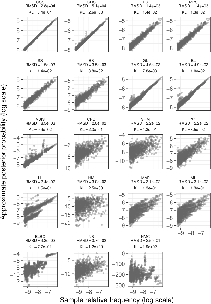
Broadly speaking, there is concordance between the performance of approximations whether measured by KL divergence or RMSD (Figures 2, 3). This is reassuring, as a good approximation should estimate the marginal likelihoods well, which should result in good approximations to the posterior, and thus good estimation of the split probabilities. We also find that the methods do a better job approximating the marginal likelihood of more probable trees than less probable trees (seen as triangular shapes of scatter points in Figure 3). However, even methods that lead to notable scatter between truth and approximation, such as PPD, can yield quite good estimates of the probabilities of splits. Additionally, if the only quantity of interest is the 50% majority-rule consensus tree, then even methods that estimate the marginal likelihood quite poorly can lead to reasonable trees (Figure 5). To get the same consensus tree, a method must merely place the same splits in the upper 50% range of posterior probability, so this measure can hide a substantial amount of variability in the estimated marginal likelihoods.

Figure 2. The posterior probabilities of all the splits observed in DS5 for a single replicate. MrBayes posteriors are plotted on the x-axis versus the denoted approximation on the y-axis. Points are colored by the thresholds we discuss: RMSD

<

0.01 is a good approximation (green), 0.01

\leq

RMSD

<

0.05 is a potentially acceptable approximation (yellow), and RMSD

\geq

0.05 is poor (red). Panels are ordered by RMSD in increasing order.

Refer to caption — Figure 3. The approximate posterior probabilities of the topologies in DS5 versus the ground truth posterior probabilities from MrBayes, plotted on the log scale for clarity. The rank-ordering of the methods is closest to average for DS5. Results are for a single run of each method. Panels are ordered by RMSD in increasing order.

Speed

Fast methods can give accurate results, while slow methods need not be accurate (Figure 4). Indeed, GL is very fast to compute and gives good results, GLIS is only slightly slower and gives excellent results, while NS is slow to compute and gives rather bad results for this problem.

Method speed is primarily determined by the amount of sampling performed by the method: the more sampling required by a method, the slower it is. The fastest methods are deterministic and do not perform sampling at all, with MAP and ML being the fastest of the 19, requiring only optimization. There is a minor added computational cost of calculating additional derivatives of the phylogenetic likelihood function (here purely the derivatives with respect to branch lengths) in the case of the Laplus approximations. The calculation of the ELBO is slightly slower due to the cost of optimizing the variational parameters through stochastic gradient ascent. The next jump in speed is to methods that perform importance sampling. The single-chain methods are very consistent in time requirements since the computation time is largely dominated by the MCMC. They are notably slower than the importance sampling methods, because MCMC here used one million samples per tree, while we use 10,000 for importance sampling. The slowest methods require running multiple MCMC chains, and aside from GSS time requirements are essentially identical between these methods. We used 50 power posteriors in our analysis of stepping stone and path sampling methods, and as expected we find that they are very nearly 50 times slower than the single-chain methods. The consistency of the number of chains and the time requirement of the method clearly demonstrates that the largest computational effort is in the MCMC. It is worth noting, though, that after an MCMC analysis has run (power posteriors or single chains), any appropriate method can be used to post-process the chains and calculate the marginal likelihood, as MrBayes does with arithmetic and harmonic means. As an implementation detail of this study, every single-chain method uses the same MCMC samples to estimate the marginal likelihood and similarly, the power posterior-based methods use the same power posterior samples.

Figure 4. Average RMSD of splits in the approximate posterior against running time. Text denotes method used, while superscripts label applications to individual datasets. Four methods are omitted for visual clarity: MAP is essentially identical to ML, BL is nearly identical to GL, and PS and MPS are both similar to SS. The horizontal dashed and solid lines depict RMSDs of 0.01 and 0.05 respectively. The RMSD is calculated using the average marginal likelihood of each tree from each of 10 replicate analyses. The running time is calculated using the average running time of each tree from each of 10 replicate analyses.

Monte Carlo error

No method to estimate the posterior probability of a tree is without sources of error. Monte Carlo error is a feature of all of sampling-based methods we benchmarked, including the methods using at least one MCMC chain and importance sampling methods (marked by asterisks in Table 1). For these methods, and the variational approach (which uses stochastic optimization with noisy gradient estimates and thus also has inter-run variability) we ran 10 replicate analyses (Figure S11). Interestingly, we find that the inter-run variability of the methods is correlated with the goodness of the estimates (and hence the rank-orderings of the methods are similar in Figure S11 and Figure 1). In discussing how well the methods approximate the posterior distribution of trees, to diminish the effects of Monte Carlo error, we use the average estimated marginal likelihood across the replicate analyses.

Summary trees

The accuracy of summary trees was correlated as expected with the accuracy of the posterior estimate on splits (Figure 5). We use majority-rule consensus trees (Margush and McMorris 1981), where a split appears in the consensus tree only if it appears in tree topologies whose posterior probabilities sum to at least 0.5. Thus for two approximate posteriors to produce the same summary tree, they must only agree on whether a split probability is above or below this threshold, meaning this is a less sensitive measure of how good an approximate posterior is than RMSD or KL. In Figure 5, we show consensus trees for methods representing good approximations (RMSD $<$ 0.01), acceptable approximations (0.01 $\leq$ RMSD $<$ 0.05), and poor approximations (RMSD $\geq$ 0.05) for DS5 for a single run of each method. In this run, every good approximate posterior and most (0.59%) acceptable approximate posteriors produced a consensus tree identical to the golden run consensus tree. A small portion (0.25%) of poor approximate posteriors also produced identical consensus trees.

Figure 5. Majority rule consensus trees DS5 based on four sources for posterior probabilities of trees. Each taxon is assigned a unique color and the branch leading to that taxon is colored the same in all 4 trees to show differences. The golden run and GLIS trees are identical, while the tree for ML has a Robinson-Foulds distance of 4 to those trees and the tree for NMC a distance 14 (and 10 from the ML tree). Nodes with red circles denote parts of the tree different from the golden run tree.

Discussion

In this paper, we present the most comprehensive benchmark to date of methods for computing marginal likelihoods of phylogenetic tree topologies. A number of estimators we benchmark are well known to the phylogenetics community, namely power posterior methods (e.g. GSS) and the HM. We also include estimators that have been used less frequently in phylogenetics and are mainly more recent proposals: CPO, NS, and the SHM. Three estimators, BS, PPD, and NMC, to the best of our knowledge, have not previously been used in phylogenetics. Variational approaches have been proposed for models of heterogeneous stationary frequencies (Dang and Kishino 2018), otherwise intractable phylogenetic models (Jojic et al. 2004; Wexler and Geiger 2007; Cohn et al. 2010), and to fit approximations to distributions on trees (Zhang and Matsen 2018), but to our knowledge this is the first application of the ELBO to phylogenetic model comparison. One goal of this paper is to find methods that could work well with MCMC-free tree exploration approaches like PT, which requires evaluating the marginal likelihoods of hundreds or thousands of topologies. Aside from the ELBO, none of the above methods are fast enough to be suitable for this purpose. To this end, we develop the Laplus approximations and importance sampling methods based on Laplus and variational approximations. We also consider simply using the ML and the MAP.

Choosing a method to use in practical scenarios

As expected, methods differ drastically in runtime in proportion to the required Monte Carlo sampling effort. The fastest methods took less than one second per topology on all datasets analyzed, while the slowest took over 10,000. Perhaps surprisingly, there is no general tradeoff between speed and accuracy; while the slowest methods are among the most accurate, there are fast methods that are as good. We break the methods down into four categories: slow, moderately slow, fast, and ultrafast, and will now reviewing the methods by category—from slow and well-known to fast and novel—highlighting the best performers and their use cases.

At the slow end of the spectrum, we find that the tried-and-true power posterior methods perform quite well, with GSS providing the best (and most precise) estimates of all 19 methods. The boost in performance compared from GSS relative to the other power posterior methods comes at the cost of a marginal increase in computation time due to the estimation and multiple evaluation of the reference distribution. The approximations produced by PS, MPS, and SS are all acceptable (i.e. RMSD $<0.05$ ), with most of approximations falling into the good category (i.e. RMSD $<0.01$ ), and are similar in terms of speed, accuracy, and precision. The power posterior methods remain the best general-purpose tools for phylogenetic model comparisons, though they are certainly too slow to explore the tree space produced by PT.

In the middle of the speed axis, we find that BS is the most promising method, with performance that is on par with PS, MPS, and SS. As BS requires an order of magnitude less time than these power posterior-based methods, if it is extended to incorporate sampling trees (perhaps following Baele et al. 2015) it could become a valuable general-purpose model selection tool. The other estimators in this category span from poor to acceptable. The HM is a very bad estimator of the marginal likelihood, though the related SHM produces posteriors that are acceptable. Two other methods similar in spirit to the HM, CPO (a harmonic sitewise approach) and PPD (a sitewise arithmetic approach), both perform much better than the HM or the SHM. NS would appear to be an unwise choice for estimating the marginal likelihoods of topologies, as it produces poor approximate posteriors. We note that this is a somewhat different application of NS than the recent work by Maturana Russel et al. 2018, who report better results of using NS when averaging over (ultrametric) trees.

GLIS is the best fast method, and one of the best among the 19. With 10,000 samples, it produces estimates of the marginal likelihood on par with GSS while working three orders of magnitude more quickly. VBIS produces marginal likelihoods almost as good but is somewhat slower. The ELBO, while faster than either GLIS or VBIS (which uses the variational approximation as the importance distribution) is notably worse. It is possible that this approach suffers from getting stuck in local minima, and that multiple starting points could improve its performance, and consequently the performance of VBIS. The worst method in this speed category with regards to accuracy, indeed of all 19 methods, is NMC.

Among the ultrafast methods, the best candidate is GL. All the Laplus approximations are capable of yielding quite good estimates of the posterior distribution on trees, though they are quite variable in performance between methods, and LL can produce poor approximate posteriors. MAP and ML are faster than any of the Laplus approximations, but are not as good. However, the success of all of these methods is truly remarkable. Empirical posterior distributions on branch lengths are clearly not point-masses, and yet simply normalizing the unnormalized posterior at the maximum outperforms 6 of the 19 tested methods. The success of the Laplus approximations suggests that our assumption of independence of branch lengths may not be too unreasonable, though their rather large inter-dataset variability and the improvement from importance sampling (i.e. GLIS) suggest that relaxing this assumption may improve performance.

Future directions

We restricted ourselves here to fixed-topology inference under the simplest substitution model. Future work should generalize beyond this simplest model to obtain a marginal likelihood across all continuous model parameters for more complex models.

Another direction for future work is to investigate the effect of modelling correlation between model parameters, including within branch lengths. Although our preliminary results suggest that correlation between branch lengths is not strong, this assumption is not likely to hold for other parameters in more sophisticated models, such as the coalescent model in which the tree height/length is likely to be positively correlated with parameters governing population dynamics.

Another future research avenue is to find some way to reduce the inter-dataset variability of the Laplus approximations. While this class of methods does very well on some datasets, in others there is a subset of topologies that present difficulties, possibly due to short branches with odd posterior distributions. The problems of identifying these branches and what to do with them remain open, but solving them may greatly improve the performance of the Laplus approximation.

For fixed topology models, our results suggest bridge sampling is an accurate estimator that does not require as much compute time as the power posterior-based methods. To apply this method more broadly to the phylogenetic field we must develop novel bridge sampling proposal distributions, perhaps modeling correlation between parameters other than branch lengths, and more importantly proposals that sample a variety of tree topologies. However there has been some work on developing approximations of the posterior probability of trees (Höhna and Drummond 2011; Larget 2013; Zhang and Matsen 2018), notably within the GSS framework (Baele et al. 2015).

Another avenue for research would be to develop a diagnostic to determine an appropriate number of power posteriors that is required to accurately estimate marginal likelihoods. Preliminary analyses have shown that the estimates calculated from 100 power posteriors were similar to estimates using 50 steps, it is however possible that fewer steps would be sufficient.

Perhaps more enticing, though, is the prospect of integrating one of the fast or ultrafast methods with PT. PT currently uses ML—the fastest method of the 19—because speed is important, but GL is comparable in speed while producing much better marginal likelihood estimates, so its inclusion in PT is worth investigating. For the added time cost of drawing samples and calculating additional likelihoods, GLIS achieves an even more impressive estimate of the marginal likelihood than GL. However, given that PT explores far more trees than it eventually stores, this added time cost is almost certainly prohibitive, unless the number of importance samples can be drastically reduced. Nonetheless, once PT has found a set of high-likelihood trees, it seems prudent to use GLIS on this set to produce the final approximate posterior.

Acknowledgements

This research funded by National Science Foundation grant CISE-1561334, CISE-1564137 and National Institutes of Health grant U54-GM111274. The research of FAM was supported in part by a Faculty Scholar grant from the Howard Hughes Medical Institute and the Simons Foundation. Computational facilities were provided to MF by the UTS eResearch High Performance Computer Cluster.

References

Aberer et al. [2015] Andre J Aberer, Alexandros Stamatakis, and Fredrik Ronquist. An efficient independence sampler for updating branches in Bayesian Markov chain Monte Carlo sampling of phylogenetic trees. Systematic Biology, 65(1):161–176, 2015.
Baele et al. [2012] Guy Baele, Philippe Lemey, Trevor Bedford, Andrew Rambaut, Marc A Suchard, and Alexander V Alekseyenko. Improving the accuracy of demographic and molecular clock model comparison while accommodating phylogenetic uncertainty. Molecular Biology and Evolution, 29(9):2157–2167, 2012.
Baele et al. [2015] Guy Baele, Philippe Lemey, and Marc A Suchard. Genealogical working distributions for Bayesian model testing with phylogenetic uncertainty. Systematic Biology, 65(2):250–264, 2015.
Cohn et al. [2010] Ido Cohn, Tal El-Hay, Nir Friedman, and Raz Kupferman. Mean field variational approximation for continuous-time Bayesian networks. Journal of Machine Learning Research, 11(Oct):2745–2783, 2010.
Dang and Kishino [2018] Tung Dang and Hirohisa Kishino. Stochastic variational inference for Bayesian phylogenetics: A case of CAT model. bioRxiv, page 358747, 2018.
Drummond et al. [2012] Alexei J Drummond, Marc A Suchard, Dong Xie, and Andrew Rambaut. Bayesian phylogenetics with BEAUti and the BEAST 1.7. Molecular Biology and Evolution, 29(8):1969–1973, 2012.
Fan et al. [2010] Yu Fan, Rui Wu, Ming-Hui Chen, Lynn Kuo, and Paul O Lewis. Choosing among partition models in Bayesian phylogenetics. Molecular Biology and Evolution, 28(1):523–532, 2010.
Fourment and Holmes [2014] Mathieu Fourment and Edward C Holmes. Novel non-parametric models to estimate evolutionary rates and divergence times from heterochronous sequence data. BMC Evolutionary Biology, 14(1):163, 2014.
Friel and Pettitt [2008] Nial Friel and Anthony N Pettitt. Marginal likelihood estimation via power posteriors. Journal of the Royal Statistical Society: Series B (Statistical Methodology), 70(3):589–607, 2008.
Friel et al. [2014] Nial Friel, Merrilee Hurn, and Jason Wyse. Improving power posterior estimation of statistical evidence. Statistics and Computing, 24(5):709–723, 2014.
Gelman and Meng [1998] Andrew Gelman and Xiao-Li Meng. Simulating normalizing constants: from importance sampling to bridge sampling to path sampling. Statistical Science, pages 163–185, 1998.
Gelman et al. [1996] Andrew Gelman, Xiao-Li Meng, and Hal Stern. Posterior predictive assessment of model fitness via realized discrepancies. Statistica Sinica, pages 733–760, 1996.
Gronau et al. [2017] Quentin F Gronau, Alexandra Sarafoglou, Dora Matzke, Alexander Ly, Udo Boehm, Maarten Marsman, David S Leslie, Jonathan J Forster, Eric-Jan Wagenmakers, and Helen Steingroever. A tutorial on bridge sampling. Journal of Mathematical Psychology, 81:80–97, 2017.
Guindon [2010] Stéphane Guindon. Bayesian estimation of divergence times from large sequence alignments. Molecular Biology and Evolution, 27(8):1768–1781, 2010.
Hammersley and Handscomb [1964] John Michael Hammersley and David Christopher Handscomb. General principles of the Monte Carlo method. In Monte Carlo Methods, pages 50–75. Springer, 1964.
Hans et al. [2007] Chris Hans, Adrian Dobra, and Mike West. Shotgun stochastic search for “large p” regression. Journal of the American Statistical Association, 102(478):507–516, 2007.
Höhna and Drummond [2011] Sebastian Höhna and Alexei J Drummond. Guided tree topology proposals for Bayesian phylogenetic inference. Systematic Biology, 61(1):1–11, 2011.
Höhna et al. [2008] Sebastian Höhna, Michael Defoin-Platel, and Alexei J Drummond. Clock-constrained tree proposal operators in Bayesian phylogenetic inference. In 8th IEEE International Conference on BioInformatics and BioEngineering (BIBE 2008), pages 1–7, Athens, Greece, 2008.
Jojic et al. [2004] Vladimir Jojic, Nebojsa Jojic, Chris Meek, Dan Geiger, Adam Siepel, David Haussler, and David Heckerman. Efficient approximations for learning phylogenetic HMM models from data. Bioinformatics, 20(suppl_1):i161–i168, 2004.
Jukes and Cantor [1969] T.H Jukes and C.R. Cantor. Evolution of protein molecules. In Mammalian Protein Metabolism, pages 21–32. Academic Press, New York, 1969.
Kass and Raftery [1995] Robert E Kass and Adrian E Raftery. Bayes factors. Journal of the American Statistical Association, 90(430):773–795, 1995.
Kucukelbir et al. [2015] Alp Kucukelbir, Rajesh Ranganath, Andrew Gelman, and David Blei. Automatic variational inference in Stan. In Advances in Neural Information Processing Systems, pages 568–576, 2015.
Lakner et al. [2008] Clemens Lakner, Paul Van Der Mark, John P Huelsenbeck, Bret Larget, and Fredrik Ronquist. Efficiency of Markov chain Monte Carlo tree proposals in Bayesian phylogenetics. Systematic Biology, 57(1):86–103, 2008.
Larget [2013] Bret Larget. The estimation of tree posterior probabilities using conditional clade probability distributions. Systematic Biology, 62(4):501–511, 2013.
Lartillot and Philippe [2006] Nicolas Lartillot and Hervé Philippe. Computing Bayes factors using thermodynamic integration. Systematic Biology, 55(2):195–207, 2006.
Lenkoski and Dobra [2011] Alex Lenkoski and Adrian Dobra. Computational aspects related to inference in Gaussian graphical models with the G-Wishart prior. Journal of Computational and Graphical Statistics, 20(1):140–157, 2011.
Lewis et al. [2013] Paul O Lewis, Wangang Xie, Ming-Hui Chen, Yu Fan, and Lynn Kuo. Posterior predictive Bayesian phylogenetic model selection. Systematic Biology, 63(3):309–321, 2013.
Lewis et al. [2016] Paul O Lewis, Ming-Hui Chen, Lynn Kuo, Louise A Lewis, Karolina Fučíková, Suman Neupane, Yu-Bo Wang, and Daoyuan Shi. Estimating Bayesian phylogenetic information content. Systematic Biology, 65(6):1009–1023, 2016.
Margush and McMorris [1981] Timothy Margush and Fred R McMorris. Consensusn-trees. Bulletin of Mathematical Biology, 43(2):239–244, 1981.
Maturana Russel et al. [2018] Patricio Maturana Russel, Brendon J Brewer, Steffen Klaere, and Remco R Bouckaert. Model selection and parameter inference in phylogenetics using nested sampling. Systematic Biology, June 2018. doi: 10.1093/sysbio/syy050.
Meng and Wong [1996] Xiao-Li Meng and Wing Hung Wong. Simulating ratios of normalizing constants via a simple identity: a theoretical exploration. Statistica Sinica, pages 831–860, 1996.
Moler and Van Loan [1978] C Moler and C Van Loan. Nineteen dubious ways to compute the exponential of a matrix. SIAM Rev., 20(4):801–836, October 1978.
Moler and Van Loan [2003] C Moler and C Van Loan. Nineteen dubious ways to compute the exponential of a matrix, Twenty-Five years later. SIAM Rev., 45(1):3–49, 2003.
Newton and Raftery [1994] Michael A Newton and Adrian E Raftery. Approximate Bayesian inference with the weighted likelihood bootstrap. Journal of the Royal Statistical Society. Series B (Methodological), pages 3–48, 1994.
Ogata [1989] Yosihiko Ogata. A Monte Carlo method for high dimensional integration. Numerische Mathematik, 55(2):137–157, 1989.
Overstall and Forster [2010] Antony M Overstall and Jonathan J Forster. Default Bayesian model determination methods for generalised linear mixed models. Computational Statistics & Data Analysis, 54(12):3269–3288, 2010.
Owen [2013] Art B. Owen. Monte Carlo Theory, Methods and Examples. 2013. https://statweb.stanford.edu/~owen/mc/.
Raftery and Banfield [1991] Adrian E Raftery and Jeffrey D Banfield. Stopping the Gibbs sampler, the use of morphology, and other issues in spatial statistics (Bayesian image restoration, with two applications in spatial statistics)–(discussion). Annals of the Institute of Statistical Mathematics, 43(1):p32–43, 1991.
Ranganath et al. [2014] Rajesh Ranganath, Sean Gerrish, and David Blei. Black box variational inference. In Artificial Intelligence and Statistics, pages 814–822, 2014.
Reis and Yang [2011] Mario dos Reis and Ziheng Yang. Approximate likelihood calculation on a phylogeny for Bayesian estimation of divergence times. Molecular Biology and Evolution, 28(7):2161–2172, 2011.
Ronquist et al. [2012] Fredrik Ronquist, Maxim Teslenko, Paul Van Der Mark, Daniel L Ayres, Aaron Darling, Sebastian Höhna, Bret Larget, Liang Liu, Marc A Suchard, and John P Huelsenbeck. MrBayes 3.2: efficient Bayesian phylogenetic inference and model choice across a large model space. Systematic Biology, 61(3):539–542, 2012.
Skilling [2004] John Skilling. Nested sampling. In AIP Conference Proceedings, volume 735, pages 395–405. AIP, 2004.
Skilling et al. [2006] John Skilling et al. Nested sampling for general Bayesian computation. Bayesian Analysis, 1(4):833–859, 2006.
Thorne et al. [1998] Jeffrey L Thorne, Hirohisa Kishino, and Ian S Painter. Estimating the rate of evolution of the rate of molecular evolution. Molecular Biology and Evolution, 15(12):1647–1657, 1998.
Tierney and Kadane [1986] Luke Tierney and Joseph B Kadane. Accurate approximations for posterior moments and marginal densities. Journal of the American Statistical Association, 81(393):82–86, 1986.
Vehtari et al. [2017] Aki Vehtari, Andrew Gelman, and Jonah Gabry. Practical Bayesian model evaluation using leave-one-out cross-validation and WAIC. Statistics and Computing, 27(5):1413–1432, 2017.
Wexler and Geiger [2007] Ydo Wexler and Dan Geiger. Variational upper bounds for probabilistic phylogenetic models. In Annual International Conference on Research in Computational Molecular Biology, pages 226–237. Springer, 2007.
Whidden and Matsen IV [2015] Chris Whidden and Frederick A Matsen IV. Quantifying MCMC exploration of phylogenetic tree space. Systematic Biology, 64(3):472–491, 2015.
Whidden et al. [2018] Chris Whidden, Brian Claywell, Thayer Fisher, Andy Magee, Mathieu Fourment, and Frederick A Matsen IV. Systematic exploration of the high likelihood density set of phylogenetic trees. 2018.
Xie et al. [2010] Wangang Xie, Paul O Lewis, Yu Fan, Lynn Kuo, and Ming-Hui Chen. Improving marginal likelihood estimation for Bayesian phylogenetic model selection. Systematic Biology, 60(2):150–160, 2010.
Zhang and Matsen [2018] C. Zhang and F. A. Matsen, IV. Generalizing tree probability estimation via Bayesian networks. ArXiv e-prints, May 2018.

1. Methods

In the Bayesian framework, the marginal likelihood or evidence of data $D$ conditioned on model $\tau$ with associated parameters $\bm{\theta}=(\theta_{1},\theta_{2},\dots,\theta_{N})$ is

p(D\mid\tau)=\int p(D\mid\bm{\theta},\tau)p(\bm{\theta}\mid\tau)d\bm{\theta},

where $p(D\mid\bm{\theta},\tau)$ is the probability of the data given parameters $\bm{\theta}$ , $p(\bm{\theta}\mid\tau)$ is the prior on $\bm{\theta}$ , and the integral is of dimension N.

Dependence on model $\tau$ is suppressed in the rest of the document to simplify notation.

1.1. Laplace method

1.1.1. Classical Laplace

The Laplace method [Tierney and Kadane 1986] approximates the marginal likelihood by approximating the posterior distribution using a multivariate normal distribution with mean equal to the maximum a posteriori estimates $\bm{\tilde{\theta}}$ , and covariance $\tilde{\Sigma}=(-H)^{-1}$ where $H$ is the Hessian matrix of second derivatives of $\log(p(D\mid\bm{\theta})p(\bm{\theta}))$ . Specifically, let us define $l(\bm{\theta})=\log(p(D\mid\bm{\theta})p(\bm{\theta}))$ and Taylor-expand $l(\bm{\theta})$ around $\bm{\tilde{\theta}}$ . Exponentiating this quadratic approximation leads to a normal distribution with $\bm{\tilde{\mu}}=\bm{\tilde{\theta}}$ and $\tilde{\Sigma}=-H^{-1}$ . Integrating the normal distribution yields the Laplace marginal likelihood estimator

\hat{p}_{L}(D)\approx(2\pi)^{d/2}\det(\tilde{\Sigma})^{1/2}p(D\mid\bm{\tilde{\theta}})p(\bm{\tilde{\theta}}),

where $\det(\tilde{\Sigma})$ is the determinant of the covariance matrix.

Unfortunately, the above normal approximation is not always accurate in practice. In our specific phylogenetic setting, the positivity of branch lengths creates problems for the normal approximation. It is however possible to improve the normal approximation of the posterior and the Laplace method if we transform each variable $\theta_{i}$ using a one-to-one twice differentiable function $g$ such as $\theta_{i}=g(z_{i})$ and $z_{i}=g^{-1}(\theta_{i})$ . Applying the chain rule, the Hessian of the posterior for the transformed parameters is

H_{i,j}^{z}=\frac{\partial^{2}l}{\partial z_{i}\partial z_{j}}=\begin{cases}\frac{\partial l}{\partial\theta_{i}}\frac{\partial^{2}\theta_{i}}{\partial z_{i}^{2}}+H_{ii}\left(\frac{\partial\theta_{i}}{\partial z_{i}}\right)^{2}&\text{for }i=j,\\ H_{ij}\frac{\partial\theta_{i}}{\partial z_{i}}\frac{\partial\theta_{j}}{\partial z_{j}}&\text{otherwise}.\end{cases}

The transformation requires an adjustment to account for the distortion of the distribution hence insuring that the distribution integrates to 1. Therefore, given $\bm{z}\sim\mathcal{N}(\bm{\mu},\bm{\Sigma})$ the density of $\bm{\theta}$ is

p(\bm{\theta})=\mathcal{N}(g^{-1}(\bm{\theta})\mid\bm{\mu},\bm{\Sigma})\,|\det J_{g^{-1}}(\bm{\theta})|,

where $|\det J_{g^{-1}}(\bm{\theta})|$ is the absolute value of the determinant of the Jacobian matrix evaluated at $\bm{\theta}$ . However, we find in practice that some branch length posteriors are monotonically decreasing functions with modes at 0, and thus the transformation approach is not sufficient to make the normal approximation accurate.

1.1.2. The Laplus approximations

However, while some transformations may work well for a branch or subset of branches, we find in practice that there is no one transformation that works well for all branches on a tree. As an alternative we use a family of approximations inspired by the Laplace that we call the Laplus approximations (in recognition of the fact that they are like the Laplace but designed for parameters on $\mathbb{R}^{+}$ ). We share with the Laplace approximation the assumption that the posterior is concentrated around the mode, $\bm{\tilde{\theta}}$ . Unlike the Laplace approximation, we assume that branch lengths are mutually independent, such that we can make the approximation

p(\bm{\theta}\mid\tau,D)\approx\prod_{i}q(\theta_{i};\bm{\phi}_{i})

Here $q$ is a parametric distribution with known normalizing constant (such as the gamma distribution) that we will use to approximate the posterior distributions for each branch. For a given branch, $\bm{\phi}_{i}$ are the parameters of $q$ that approximate the marginal posterior of that branch. Let $C$ be a constant such that

p(\bm{\theta}\mid\tau,D)=C\times p(D\mid\tau,\bm{\theta})p(\bm{\theta})

That is, $C$ is the inverse of the marginal likelihood that we seek to estimate, and using our approximation above,

C=\frac{p(\bm{\theta}\mid\tau,D)}{p(D\mid\tau,\bm{\theta})p(\bm{\theta})}\approx\frac{\prod_{i}q(\theta_{i};\bm{\phi}_{i})}{p(D\mid\tau,\bm{\theta})p(\bm{\theta})}

Finally, by applying this equation at the posterior mode, our resulting estimate of the marginal likelihood is

\hat{p}_{\text{Laplus}}(D)=\hat{C}^{-1}=\frac{p(D|\bm{\tilde{\theta}})p(\bm{\tilde{\theta}})}{\prod_{i}q(\tilde{\theta}_{i};\bm{\phi}_{i})}

The general procedure for the Laplus approximations is similar regardless of parametric distributional family assumption $q$ . Our goal is to take the joint MAP estimates of the branch lengths $\bm{\tilde{\theta}}$ and the vector of second derivatives of the log-posterior $(\frac{\partial^{2}l}{\partial\theta_{1}^{2}},\frac{\partial^{2}l}{\partial\theta_{2}^{2}},\dots,\frac{\partial^{2}l}{\partial\theta_{n}^{2}})$ and find the parameters of our approximating distributions for each branch, $\bm{\phi}_{i}$ , by matching modes and second derivatives of the approximating and posterior distributions of branch lengths. The complete procedure is written here algorithmically.

(1)

Find the (joint) MAP branch lengths, $\bm{\tilde{\theta}}=(\tilde{\theta}_{1},\tilde{\theta}_{2},\dots,\tilde{\theta}_{n})$

(2)

for $i$ in $1:n$

(i)

Compute $\frac{\partial^{2}l}{\partial\theta_{i}^{2}}$ , the second derivative of the log unnormalized posterior with respect to the $i^{\textnormal{th}}$ branch

(ii)

Find parameters of $\bm{\phi}_{i}$ by solving

	$\displaystyle\frac{d^{2}}{dx^{2}}\log(q(x;\bm{\phi}_{i}))$	$\displaystyle=\frac{\partial^{2}l}{\partial\theta_{i}^{2}}\Big\|_{\theta_{i}=\tilde{\theta}_{i}}$
	$\displaystyle\text{mode}(q(x;\bm{\phi}_{i}))$	$\displaystyle=\tilde{\theta}_{i}$

(iii)

Catch exceptions

(3)

Compute the marginal likelihood as $\hat{p}_{\text{Laplus}}(D)=\frac{p(D|\bm{\tilde{\theta}})p(\bm{\tilde{\theta}})}{\prod_{i}q(\tilde{\theta}_{i};\bm{\phi}_{i})}$

Exceptions occur when elements of $\bm{\phi}_{i}$ are outside of the domain of support, when $H_{ii}$ is nonnegative (so the posterior has a mode at 0), or when elements of $\bm{\phi}_{i}$ are otherwise suspect (such as producing particularly high-variance distributions with very short branches). Exceptions and their handling depend on the distributional assumption, and so we describe exception handling in the section for each distribution individually. We consider three choices for $q$ , the gamma distribution, the Beta^′ distribution, and the lognormal distribution. Since the Laplus method is not derived through a Taylor expansion of the unnormalised posterior, it is not subject to some of the assumptions required by Laplace’s method. Although both methods require the function to be twice differentiable, Laplace’s method assumes that the global maxima $\tilde{\bm{\theta}}$ is not at the boundary of the interval of integration so that the first derivatives vanishes at $\tilde{\bm{\theta}}$ . Zero-length branches have typically non-zero (i.e. negative) first derivatives and positive second derivatives making the Laplus method attractive. And while it is obvious that there must be some dependence between branch lengths, we find in practice that the posterior correlations between branch lengths are often quite small.

1.1.3. Gamma-Laplus

Here we seek to approximate the marginal posteriors of all branch lengths with gamma distributions. The vector $\bm{\phi}_{i}=(\alpha_{i},\beta_{i})$ contains the shape and rate parameters of the gamma distribution; the log probability density function of the gamma is

\log(\text{Gamma}(x;\alpha,\beta))=\alpha\log(\beta)-\log(\Gamma(\alpha))+(\alpha-1)\log(x)-\beta x.

The first and second derivatives of the log gamma distribution with respect to $x$ are given by

	$\displaystyle\frac{d}{dx}\log(\text{Gamma}(x;\alpha,\beta))$	$\displaystyle=\frac{\alpha-1}{x}-\beta,$
	$\displaystyle\frac{d^{2}}{dx^{2}}\log(\text{Gamma}(x;\alpha,\beta))$	$\displaystyle=-\frac{\alpha-1}{x^{2}}.$

We make use of the second derivative of the log-posterior at the mode, $H_{ii}=\frac{\partial^{2}l}{\partial\theta_{i}^{2}}\Big|_{\theta_{i}=\tilde{\theta}_{i}}$ to estimate $\hat{\alpha}_{i}$ using the second derivative of the log of the gamma distribution. Then we solve for $\hat{\beta}_{i}$ using the analytic formula for gamma mode: $\tilde{\theta}_{i}=\frac{\alpha_{i}-1}{\beta_{i}}$ .

	$\displaystyle H_{ii}$	$\displaystyle=-\frac{\hat{\alpha}_{i}-1}{\tilde{\theta}_{i}^{2}}$
	$\displaystyle\hat{\alpha}_{i}$	$\displaystyle=1-\tilde{\theta}_{i}^{2}H_{ii}$
	$\displaystyle\hat{\beta}_{i}$	$\displaystyle=\frac{\hat{\alpha}_{i}-1}{\tilde{\theta}_{i}}=\frac{-\tilde{\theta}_{i}^{2}H_{ii}}{\tilde{\theta}_{i}}=-\tilde{\theta}_{i}H_{ii}$

We note two exceptions to handle with the GL approach. The first case are branches with a mode at 0, which have posteriors that are monotonically decreasing. The second case are branches that are short with oddly large variances. We detect branches of the first type by checking whether $\tilde{\theta}_{i}<\epsilon_{1}$ or $H_{ii}>=0$ . These branches are handled by fixing $\hat{\alpha_{i}}=1$ (to ensure that the approximation is monotonically decreasing) and fitting $\hat{\beta_{i}}$ directly using the log-posterior calculated at $N$ points spaced evenly (on the log-scale) between $\tilde{\theta}_{i}$ and 0.5. We detect branches of the second type by checking whether $\tilde{\theta}_{i}<\epsilon_{2}$ and $\frac{\alpha_{i}}{\beta_{i}^{2}}>0.1$ . These branches are handled by fitting $\alpha_{i},\beta_{i}$ to $N$ points spaced evenly (on the log-scale) between $\tilde{\theta}_{i}$ and 0.5, while constraining $\tilde{\theta}_{i}=\frac{\hat{\alpha}_{i}-1}{\hat{\beta}_{i}}$ (such that the mode of the approximation to be the mode of the posterior). We use $N=10$ , $\epsilon_{1}=10^{-6}$ , and $\epsilon_{2}=10^{-4}$ .

1.1.4. Beta^′-Laplus

Here we seek to approximate the marginal posteriors of all branch lengths as beta^′ distributions. In this case, the vector $\bm{\phi}_{i}=(\alpha_{i},\beta_{i})$ concatenates the shape parameters of the beta^′ distribution with log probability density function is

\log(\text{Beta}^{\prime}(x;\alpha,\beta))=-\log(B(\alpha,\beta))+(\alpha-1)\log(x)-(\alpha+\beta)\log(x+1),

where $B$ is the beta function.

The first and second derivatives of the log beta^′ distribution with respect to $x$ are given by

	$\displaystyle\frac{d}{dx}\log(\text{Beta}^{\prime}(x;\alpha,\beta))$	$\displaystyle=\frac{\alpha-1}{x}-\frac{\alpha+\beta}{x+1},$
	$\displaystyle\frac{d^{2}}{dx^{2}}\log(\text{Beta}^{\prime}(x;\alpha,\beta))$	$\displaystyle=-\frac{\alpha-1}{x^{2}}+\frac{\alpha+\beta}{(x+1)^{2}}.$

When $\alpha\leq 1$ , the beta^′ distribution collapses to a monotonically decreasing distribution. When $\alpha=1$ ,

	$\displaystyle\log(\text{Beta}^{\prime}(x;1,\beta_{i}))$	$\displaystyle=-\log(B(1,\beta_{i}))+(1-1)\log(x)-(1+\beta_{i})\log(x+1),$
	$\displaystyle\log(\text{Beta}^{\prime}(x;1,\beta_{i}))$	$\displaystyle=-\log(B(1,\beta_{i}))-(1+\beta_{i})\log(x+1),$
	$\displaystyle\frac{d}{dx}\log(\text{Beta}^{\prime}(x;1,\beta_{i}))$	$\displaystyle=-\frac{1+\beta_{i}}{x+1}.$

We make use of the second derivative at the mode, $H_{ii}=\frac{\partial^{2}l}{\partial\theta_{i}^{2}}\Big|_{\theta_{i}=\tilde{\theta}_{i}}$ to estimate $\hat{\beta}_{i}$ . Then we solve for $\hat{\alpha}_{i}$ using the fact that $\tilde{\theta}_{i}=\frac{\hat{\alpha}_{i}-1}{\hat{\beta}_{i}+1}$ .

	$\displaystyle H_{ii}$	$\displaystyle=-\frac{\hat{\alpha}_{i}-1}{\tilde{\theta}_{i}^{2}}+\frac{\hat{\alpha}_{i}+\hat{\beta}_{i}}{(\tilde{\theta}_{i}+1)^{2}}$
		$\displaystyle=-\frac{1}{\tilde{\theta}_{i}}\frac{\hat{\alpha}_{i}-1}{\frac{\hat{\alpha}_{i}-1}{\hat{\beta}_{i}+1}}+\frac{1}{\tilde{\theta}_{i}+1}\frac{\hat{\alpha}_{i}+\hat{\beta}_{i}}{\frac{\hat{\alpha}_{i}+\hat{\beta}_{i}}{\hat{\beta}_{i}+1}}$
		$\displaystyle=-\frac{1}{\tilde{\theta_{i}}}(\hat{\beta}_{i}+1)+\frac{1}{\tilde{\theta}_{i}+1}(\hat{\beta}_{i}+1)$
		$\displaystyle=(\hat{\beta}_{i}+1)\Big(\frac{1}{\tilde{\theta}_{i}+1}-\frac{1}{\tilde{\theta}_{i}}\Big)$
		$\displaystyle=\frac{\hat{\beta}_{i}+1}{\tilde{\theta}_{i}(\tilde{\theta}_{i}+1)}$
	$\displaystyle\hat{\beta}_{i}$	$\displaystyle=-H_{ii}(\tilde{\theta}_{i}+1)\tilde{\theta}_{i}-1$
	$\displaystyle\hat{\alpha}_{i}$	$\displaystyle=\tilde{\theta}_{i}(\hat{\beta}_{i}+1)+1.$

We note two exceptions to handle with the BL approach. To start, we check if $\hat{\beta}_{i}<0$ , which implies $H_{ii}>0$ , meaning the posterior should be monotonically decreasing. In this case, we set $\hat{\alpha}_{i}=1$ and use the equations outlined below to fit $\hat{\beta}_{i}$ . We then check if $\hat{\beta}_{i}<2$ , in which case our approximate posterior has suspiciously high variance, in which case we fit $\alpha_{i},\beta_{i}$ to $N$ points spaced evenly (on the log-scale) between $\tilde{\theta}_{i}$ and 0.5, while constraining $\tilde{\theta}_{i}=\frac{\hat{\alpha}_{i}-1}{\hat{\beta}_{i}+1}$ (such that the mode of the approximation to be the mode of the posterior).

When we set $\hat{\alpha}_{i}=1$ we can use the first derivative of the log-posterior, $\nabla_{i}=\frac{\partial l}{\partial\theta_{i}}\Big|_{\theta_{i}=\tilde{\theta}_{i}}$ , to fit $\hat{\beta}_{i}$ :

	$\displaystyle\nabla_{i}$	$\displaystyle=-\frac{1+\hat{\beta}_{i}}{\tilde{\theta}_{i}+1},$
	$\displaystyle\hat{\beta_{i}}$	$\displaystyle=-\nabla_{i}(\tilde{\theta}_{i}+1)-1.$

1.1.5. Lognormal-Laplus

Here we seek to approximate the marginal posteriors of all branch lengths as lognormal distributions. The vector $\bm{\phi}_{i}=(\mu_{i},\sigma_{i})$ concatenates the mean and standard deviation parameters of the lognormal distribution with log probability density function

\log(\text{Lognormal}(x;\mu_{i},\sigma_{i}))=-\frac{\log(2\pi)}{2}-\log(x)-\log(\sigma_{i})-\frac{(\log(x)-\mu_{i})^{2}}{2\sigma_{i}^{2}}.

The first and second derivatives of the log lognormal distribution with respect to $x$ are given by

	$\displaystyle\frac{d}{dx}\log(\text{Lognormal}(x;\mu_{i},\sigma_{i}))$	$\displaystyle=-\frac{1}{x}-\frac{\log(x)-\mu_{i}}{x\sigma_{i}^{2}},$
	$\displaystyle\frac{d^{2}}{dx^{2}}\log(\text{Lognormal}(x;\mu_{i},\sigma_{i}))$	$\displaystyle=\frac{1}{x^{2}}-\frac{-\log(x)+\mu_{i}+1}{x^{2}\sigma_{i}^{2}}.$

We make use of the second derivative at the mode, $H_{ii}=\frac{\partial^{2}l}{\partial\theta_{i}^{2}}\Big|_{\theta_{i}=\tilde{\theta}_{i}}$ , and the fact that $\tilde{\theta}_{i}=e^{\mu_{i}-\sigma_{i}^{2}}$ to estimate $\hat{\sigma}_{i}^{2}$ . Then we solve for $\hat{\mu}_{i}$ using the fact that $\log(\tilde{\theta}_{i})=\mu_{i}-\sigma_{i}^{2}$ .

	$\displaystyle H_{ii}$	$\displaystyle=\frac{1}{\tilde{\theta}_{i}^{2}}-\frac{-\log(\tilde{\theta}_{i})+\hat{\mu}_{i}+1}{\tilde{\theta}_{i}^{2}\hat{\sigma}_{i}^{2}}$
		$\displaystyle=\frac{1}{\tilde{\theta}_{i}^{2}}-\frac{-(\hat{\mu}_{i}-\hat{\sigma}_{i}^{2})+\hat{\mu}_{i}+1}{\tilde{\theta}_{i}^{2}\hat{\sigma}_{i}^{2}}$
		$\displaystyle=\frac{1}{\tilde{\theta}_{i}^{2}}-\frac{1}{\tilde{\theta}_{i}^{2}\hat{\sigma}_{i}^{2}}-\frac{\hat{\sigma}_{i}^{2}}{\tilde{\theta}_{i}^{2}\hat{\sigma}_{i}^{2}},$
	$\displaystyle\hat{\sigma}_{i}^{2}$	$\displaystyle=-\frac{1}{\tilde{\theta}_{i}^{2}H_{ii}},$
	$\displaystyle\hat{\mu}_{i}$	$\displaystyle=\log(\tilde{\theta}_{i})+\hat{\sigma}_{i}^{2}.$

We note two exceptions to handle with the LL approach. The first case are branches with a mode at 0, which have posteriors that are monotonically decreasing. The second case are branches that are short with oddly large variances. We nest the cases such that we first check for branches that fall in either category, checking $\tilde{\theta}_{i}<\epsilon_{1}$ or $H_{ii}>=0$ or $\hat{\mu}>5$ (which happens when $\hat{\sigma}$ is suspiciously large). As there is no parameter regime in which the lognormal is monotonically decreasing, and suspiciously high-variance branches are not fit any better by a lognormal distribution than a gamma distribution, at this point we switch to approximating branches as gamma distributions and proceed with exceptions as in the GL approach.

1.2. Importance sampling

Importance sampling uses a reference or importance distribution from which values are drawn, allowing summaries to be calculated for an unknown distribution by taking into account the importance weights (probabilities of drawing the sampled values). If $g$ is an importance distribution then

	$\displaystyle p(D)$	$\displaystyle=\int p(D\mid\bm{\theta})p(\bm{\theta})\text{d}\bm{\theta}$
		$\displaystyle=\int\frac{p(D\mid\bm{\theta})p(\bm{\theta})}{g(\bm{\theta})}g(\bm{\theta})\text{d}\bm{\theta}$
		$\displaystyle=\mathbb{E}_{g}\left(\frac{p(D\mid\bm{\theta})p(\bm{\theta})}{g(\bm{\theta})}\right).$

For a normalized density $g$ , the estimate is given by,

\hat{p}_{\text{IS}}(D)=\frac{1}{N}\sum_{i=1}^{N}\frac{p(D\mid\tilde{\bm{\theta}_{i}})p(\tilde{\bm{\theta}_{i}})}{g(\tilde{\bm{\theta}_{i}})},\tilde{\bm{\theta}}_{i}\sim g(\bm{\theta}).

For an unnormalized density $q$ , the self normalized importance sampling estimate [Owen 2013] is given by

\hat{p}_{\text{IS}}(D)=\frac{\sum_{i=1}^{N}p(D\mid\tilde{\bm{\theta}}_{i})w(\tilde{\bm{\theta}}_{i})}{\sum_{i=1}^{N}w(\tilde{\bm{\theta}}_{i})},\tilde{\bm{\theta}}_{i}\sim q(\bm{\theta}),

where $w(\tilde{\bm{\theta}}_{i})$ is the importance weight given by $w(\tilde{\bm{\theta}}_{i})=\frac{p(\tilde{\bm{\theta}}_{i})}{q(\tilde{\bm{\theta}}_{i})}$ .

1.3. Naive Monte Carlo

The simplest Monte Carlo estimator of the marginal likelihood is defined as the expected value of the likelihood with respect to the prior distribution [Hammersley and Handscomb 1964, Raftery and Banfield 1991]. The so called naive Monte Carlo (NMC) estimator can be approximated by drawing $N$ samples ${\bm{\theta}_{1},\bm{\theta}_{2},\dots,\bm{\theta}_{N}}$ from the prior distribution and calculating the arithmetic mean of the likelihood.

\hat{p}_{\text{NMC}}(D)=\frac{1}{N}\sum_{i=1}^{N}p(D\mid\tilde{\bm{\theta}_{i}}),\tilde{\bm{\theta}}_{i}\sim p(\bm{\theta}).

Although this approach is fast and unbiased, the high-likelihood region can be distant from the high-prior region. Most $\tilde{\bm{\theta}}_{i}$ s will therefore be sampled from a region of the likelihood with low probability yielding high variance [Newton and Raftery 1994].

1.4. Harmonic mean

The harmonic mean (HM) estimator only requires samples from the posterior generated by a single MCMC or other samplers and is therefore appealing to the user [Newton and Raftery 1994]. The harmonic mean estimator of marginal estimator is equivalent to an importance sampling estimator of $1/p(D)$ with importance distribution $p(\bm{\theta}\mid D)$ :

\hat{p}_{\text{HM}}(D)=\frac{1}{\frac{1}{N}\sum_{i=1}^{N}\frac{1}{p(D\mid\tilde{\bm{\theta}_{i}})}},\tilde{\bm{\theta}}_{i}\sim p(\bm{\theta}\mid D).

This estimator is unstable due to the possible occurrence of small likelihood values the estimator and hence this estimator has infinite variance. Although the Law of Large Numbers guarantees that this estimator is consistent, the number of samples required to get an accurate estimate can be prohibitively high.

1.5. Stabilized harmonic mean

Newton and Raftery 1994 also proposed the stabilized harmonic mean (SHM) estimator to address the instability of the HM estimator. The SHM estimator is based on importance sampling scheme where the importance sampling distribution is a mixture of the prior and the posterior: $p^{\star}(\bm{\theta})=\delta p(\bm{\theta})+(1-\delta)p(\bm{\theta}\mid D)$ where $\delta$ is small, such that

\hat{p}_{\text{SHM}^{*}}(D)=\frac{\sum_{i=1}^{n}\frac{p(D\mid\tilde{\bm{\theta}}_{i})}{\delta\hat{p}_{\text{SHM}^{*}}(D)+(1-\delta)p(D\mid\tilde{\bm{\theta}}_{i})}}{\sum_{i=1}^{n}\{\delta\hat{p}_{\text{SHM}^{*}}(D)+(1-\delta)p(D\mid\tilde{\bm{\theta}}_{i})\}^{-1}},\tilde{\bm{\theta}}_{i}\sim p^{\star}(\bm{\theta}).

Unfortunately this estimator requires simulating from both the posterior and prior. Newton and Raftery proposed to simulate from the posterior and assume that a further $\frac{\delta n}{(1-\delta)}$ observations are drawn from the prior, all of them with their likelihoods equal to their expected value $p(D)$ . The likelihood of the imaginary samples drawn from the prior is $p(D\mid\theta_{j})=\hat{p}_{SHM}$ for $j=1,\dots,\frac{\delta n}{1-\delta}$ . Then, the approximate marginal likelihood $\hat{p}_{\text{SHM}}(D)$ satisfies the following equation:

\hat{p}_{\text{SHM}}(D)=\frac{\frac{\delta n}{1-\delta}+\sum_{i=1}^{n}\frac{p(D\mid\tilde{\bm{\theta}}_{i})}{\delta\hat{p}_{\text{SHM}}(D)+(1-\delta)p(D\mid\tilde{\bm{\theta}}_{i})}}{\frac{\delta n}{(1-\delta)\hat{p}_{\text{SHM}}(D)}+\sum_{i=1}^{n}\{\delta\hat{p}_{\text{SHM}}(D)+(1-\delta)p(D\mid\tilde{\bm{\theta}}_{i})\}^{-1}},\tilde{\bm{\theta}}_{i}\sim p(\bm{\theta}\mid D),

which is solved by an iterative scheme that updates an initial guess of the marginal likelihood (e.g. harmonic mean estimate) until a stopping criterion is satisfied. In our implementation the recursion stops when the absolute change in $\log\hat{p}_{\text{SHM}}(D)$ is less than $10^{-7}$ . Newton and Raftery 1994 advocate $\delta=0.01$ while Lartillot and Philippe 2006 use $\delta=0.1$ . In this study we used the $\hat{p}_{\text{SHM}}$ with $\delta=0.01$ .

1.6. Bridge sampling

Bridge sampling (BS) was initially developed to estimate Bayes factors [Kass and Raftery 1995] and was more recently adapted to approximate the marginal likelihood of a single model [Overstall and Forster 2010, Gronau et al. 2017]. Following a derivation by Gronau et al. 2017, the bridge sampling estimator is derived from the following identity:

1=\frac{\int p(D\mid\bm{\theta})p(\bm{\theta})h(\bm{\theta})g(\bm{\theta})d\bm{\theta}}{\int p(D\mid\bm{\theta})p(\bm{\theta})h(\bm{\theta})g(\bm{\theta})d\bm{\theta}},

where $g(\bm{\theta})$ is the proposal distribution and $h(\bm{\theta})$ is the bridge function. The bridge function ensures that the denominator in the identity is not zero.

Multiplying both sides of the above identity by $p(D)$ the bridge sampling estimator of the marginal likelihood is

p_{\text{BS}}(D)=\frac{\int p(D\mid\bm{\theta})p(\bm{\theta})h(\bm{\theta})g(\bm{\theta})d\bm{\theta}}{\int h(\bm{\theta})g(\bm{\theta})p(\bm{\theta}\mid D)d\bm{\theta}}=\frac{\mathbb{E}_{g(\bm{\theta})}(p(D\mid\bm{\theta})p(\bm{\theta})h(\bm{\theta}))}{\mathbb{E}_{p(\bm{\theta}\mid D)}(h(\bm{\theta})g(\bm{\theta}))}.

The marginal likelihood is approximated using $n_{1}$ samples from the posterior distribution and $n_{2}$ samples from the proposal distribution

\hat{p}_{\text{BS}}(D)=\frac{1/n_{2}\sum_{i=1}^{n_{2}}(p(D\mid\tilde{\bm{\theta}_{i}})p(\tilde{\bm{\theta}}_{i})h(\tilde{\bm{\theta}}_{i}))}{1/n_{1}\sum_{j=1}^{n_{1}}h(\bm{\theta}_{j}^{*})g(\bm{\theta}_{j}^{*})},\tilde{\bm{\theta}}_{i}\sim g(\bm{\theta}),\bm{\theta}_{j}^{*}\sim p(\bm{\theta}\mid D).

Several bridge functions can be used including the so called optimal bridge function [Meng and Wong 1996]:

h(\bm{\theta})=\frac{C}{s_{1}p(D\mid\bm{\theta})p(\bm{\theta})+s_{2}p(D)g(\bm{\theta})},

where $s_{1}=n_{1}/(n_{1}+n_{2})$ and $s_{2}=n_{2}/(n_{1}+n_{2})$ and $C$ is a constant that cancels out.

The definition of the optimal bridge function depends on the marginal likelihood itself, suggesting an iterative scheme to approximate $p(D)$ starting from an initial guess, such as the HM estimate. Gronau et al. 2017 provide a detailed description of an algorithm.

1.7. Thermodynamic integration (aka path sampling, power posterior)

The thermodynamic integration estimator was introduced by Lartillot and Philippe 2006 in the phylogenetic context, borrowing ideas from path sampling [Gelman and Meng 1998] and the physics literature where a large body of research is dedicated to the estimation of normalisation constants. Lartillot and Philippe defined a path going from the prior to the unnormalised posterior $q$ using

q_{\beta}=p(D\mid\bm{\theta})^{\beta}p(\bm{\theta})

for $\beta\in[0,1]$ . The normalisation constant $Z_{\beta}$ of the tempered unnormalised posterior is therefore

Z_{\beta}=\int_{\bm{\theta}}p(D\mid\bm{\theta})^{\beta}p(\bm{\theta})d\bm{\theta}

and the log marginal likelihood of the model follows from the path sampling identity:

\log p(D)=\log Z_{1}-\log Z_{0}=\int_{0}^{1}\frac{\partial Z_{\beta}}{\partial\beta}d\beta=\int_{0}^{1}E_{\bm{\theta}\mid D,\beta}(\log p(D\mid\bm{\theta}))d\beta.

Friel and Pettitt 2008 worked on similar ideas but differ in the choice of temperature schedule and how the integral over [0,1] is approximated. Lartillot and Philippe 2006 approximate the integral using the Simpson’s rule while Friel and Pettitt 2008 applied the trapezoidal rule. The interval $\beta\in[0,1]$ is discretized such that $0=\beta_{0}<\beta_{1}<\dots<\beta_{K}=1$ and for each $\beta_{i}$ samples are drawn from $p(\bm{\theta}\mid D,\beta_{i})$ to estimate $E_{\bm{\theta}\mid D,\beta_{i}}(\log p(D\mid\bm{\theta}))$ . For example, using the trapezoidal rule the log marginal likelihood of a given model is

\log\hat{p}_{\text{PS}}(D)\approx\sum_{i=1}^{K}(\beta_{i}-\beta_{i-1})\left(\frac{E_{i-1}+E_{i}}{2}\right),

where $E_{i}=E_{\bm{\theta}\mid\beta_{i}}\log p(D\mid\bm{\theta})$ is the expectation of the log deviance at $\beta_{i}$ .

Lartillot and Philippe 2006 used equally spaced inverse temperatures between 0 and 1, while Friel and Pettitt 2008 set $\beta_{i}=(i/K)^{5}$ . It is clear that other temperature schedules can be exploited such as a schedule based on the quantiles of parametric distribution [Xie et al. 2010] (see stepping stone section) and the adaptive scheme proposed by Friel et al. 2014. Friel et al. 2014 subsequently proposed a modified trapezoidal rule that uses the variance of the samples to improve the approximation:

\log\hat{p}_{\text{MPS}}(D)\approx\sum_{i=1}^{K}(\beta_{i}-\beta_{i-1})\left(\frac{E_{i-1}+E_{i}}{2}\right)-\sum_{i=1}^{K}\frac{(\beta_{i}-\beta_{i-1})^{2}}{12}\left(V_{i}-V_{i+1}\right),

where $V_{i}=V_{\bm{\theta}\mid\beta_{i}}(\log p(D\mid\bm{\theta}))$ is the variance of the log deviance at $\beta_{i}$ .

1.8. Stepping stone

Xie et al. 2010 proposed the stepping stone (SS) algorithm that is related to the path sampling approach described in the previous section. It uses a series of distributions defining a path between the prior and posterior and therefore inherits the computational burden of path sampling. Thermodynamic integration and stepping stone differ in the choice of $\beta$ values: Xie et al. 2010 set $\beta_{1},\dots,\beta_{n}$ equal to the quantiles of a density with fixed parameters (e.g. beta distribution). This approach allows for a more intensive sampling of power posteriors with small $\beta$ values, for which the posterior is changing rapidly.

Let’s define the unnormalized power posterior distribution $q_{\beta}=p(D\mid\bm{\theta})^{\beta}p(\bm{\theta})$ and normalized power posterior distribution $p_{\beta}=\frac{q_{\beta}}{c_{\beta}}$ , where $c_{\beta}$ is the power marginal likelihood of the data. The aim of the method is to estimate the ratio $r_{\text{SS}}=c_{1.0}/c_{0.0}$ , which is equal to $c_{1.0}$ if the prior is proper. This ratio can be expanded into a series of telescopic product of ratios using intermediate power posteriors

r_{\text{SS}}=\frac{c_{1.0}}{c_{0.0}}=\prod_{k=1}^{K}\frac{c_{\beta_{k}}}{c_{\beta_{k-1}}}=\prod_{k=1}^{K}r_{\text{SS},k},

where $r_{\text{SS},k}=c_{\beta_{k}}/c_{\beta_{k-1}}$ for $k=1,\dots,K$ . Xie et al. 2010 estimate each ratio $c_{\beta_{k}}/c_{\beta_{k-1}}$ by importance sampling using $p_{\beta_{k-1}}$ as the importance distribution. Using the definition of importance sampling the $k^{th}$ ratio is

\hat{r}_{\text{SS},k}=\frac{1}{n}\sum_{i=1}^{n}\frac{p(D\mid\bm{\theta}_{k-1,i})^{\beta_{k}}}{p(D\mid\bm{\theta}_{k-1,i})^{\beta_{k-1}}}=\frac{1}{n}\sum_{i=1}^{n}p(D\mid\bm{\theta}_{k-1,i})^{\beta_{k}-\beta_{k-1}},

where $p(D\mid\theta_{k-1,i})$ is the likelihood function evaluated at $\theta_{k-1,i}$ , the $i^{th}$ MCMC sample sampled from $p_{\beta_{k-1}}$ . The product of the $K$ ratios $\hat{r}_{\text{SS},k}$ yields the estimate of the marginal likelihood

\hat{p}_{\text{SS}}=\prod_{k=1}^{K}\hat{r}_{\text{SS},k}.

1.9. Generalized stepping stone

Although stepping stone proved to be more accurate than other approaches, such as path sampling [Xie et al. 2010], sampling distributions close to the prior (i.e., small $\beta$ values) can be difficult, particularly if the prior is diffuse. Fan et al. 2010 proposed to generalize the stepping stone method using a reference distribution that approximates the posterior distribution of interest using samples from the posterior distribution to parametrize the reference distribution. The reference distribution can be independent probability densities from the same family as the prior distribution or the product of densities with the same support. In our study the priors are exponential distributions, but we used gamma distributions that are parametrized using the method of moments. The shape and rate parameters are estimated by matching the first two moments of the gamma distribution to the marginal posterior sample mean and variance.

In the same vein as the SS method, the unnormalized and normalized power posterior distributions in the generalized stepping stone (GSS) approach are

	$\displaystyle q_{\beta}$	$\displaystyle=\big(p(D\mid\bm{\theta})p(\bm{\theta})\big)^{\beta}\big(p_{0}(\bm{\theta};\bm{\phi})\big)^{1-\beta},$
	$\displaystyle p_{\beta}$	$\displaystyle=\frac{q_{\beta}}{c_{\beta}},$

where $p(D\mid\bm{\theta})$ is the likelihood function, $p(\bm{\theta})$ is the prior distribution, $p_{0}$ is the reference distribution parametrized by $\bm{\phi}$ , and $c_{\beta}$ is the (power) marginal likelihood of the data. The key difference with the SS approach is that for $\beta=0$ the power posterior is equivalent to the reference distribution.

As for the SS method, the aim of this method is to estimate the ratio $r_{\text{GSS}}=c_{1.0}/c_{0.0}$ using importance sampling. The ratio $\hat{r}_{\text{GSS},k}$ is estimated using $n$ samples from $p_{\beta_{k-1}}$ :

\hat{r}_{\text{GSS},k}=\frac{1}{n}\sum_{i=1}^{n}\left(\frac{p(D\mid\bm{\theta}_{k-1,i})p(\bm{\theta}_{k-1,i})}{p_{0}(\bm{\theta}_{k-1,i};\bm{\phi})}\right)^{\beta_{k}-\beta_{k-1}}.

Combining $\hat{r}_{\text{GSS},k}$ for all $K$ ratios yields the marginal likelihood estimator:

\hat{p}_{\text{GSS}}=\prod_{k=1}^{K}\hat{r}_{\text{GSS},k}.

1.10. Nested sampling

Nested sampling is a Monte Carlo method that aims at calculating the marginal likelihood using a change of variable [Skilling 2004, Skilling et al. 2006]. It transforms the multidimensional evidence integral over the parameter space into a more manageable one-dimensional integral over the likelihood space. Skilling defines the prior volume as $dX=p(\bm{\theta})d\bm{\theta}$ so that

(1)

X(\lambda)=\int_{\mathcal{L}(\bm{\theta})>\lambda}p(\bm{\theta})d\bm{\theta},

where $\mathcal{L}(\bm{\theta})$ is the likelihood function and the integral is taken over the region bounded by the iso-likelihood contour $\mathcal{L}(\bm{\theta})=\lambda$ . The marginal likelihood becomes a one-dimensional integral over unit range

p_{\text{NS}}(D)=\int_{0}^{1}L(X)dX,

where $L(X)$ is the inverse function of $X(\lambda)$ .

Assuming that $L(X)$ can be computed for a sequence of decreasing values $0<X_{m}<\dots<X_{0}=1$ , the unit integral can be approximated using quadrature techniques as the weighted sum:

\hat{p}_{\text{NS}}(D)\approx\sum_{i=1}^{m}L(X_{i})w_{i},

where $w_{i}=X_{i}-X_{i-1}$ .

The nested sampling algorithm uses a clever process of sampling from the prior (hence $dX$ ) and conditioning on the likelihood being above a given size (to achieve the likelihood condition of (1)) to approximate the input to such a quadrature technique [Skilling et al. 2006, Maturana Russel et al. 2018]. The algorithm is initialized with $N$ samples $\{\bm{\theta}_{1},\dots,\bm{\theta}_{N}\}$ drawn from the prior and their corresponding likelihoods are calculated $\{\mathcal{L}(\bm{\theta}_{1}),\dots,\mathcal{L}(\bm{\theta}_{N})\}$ . The sample with the lowest likelihood $L_{\min}$ is discarded from the set and replaced by a new sample $\bm{\theta}^{*}$ drawn from the prior subject to the constraint $L>L_{\min}$ . When we use the discarded point as an $X_{i}$ , the other points in the set of course satisfy the likelihood constraint. There are a variety of choices for terminating the algorithm [Maturana Russel et al. 2018]. We choose to terminate when the absolute change in $\log(\hat{p}_{\text{NS}}(D))$ is less than $10^{-6}$ .

1.11. Posterior predictive model selection

As an alternative to the marginal likelihood, the fit of a model can be assessed through the accuracy of its predictions [Gelman et al. 1996]. The probability distribution of a new data set $\tilde{D}$ having observed data set $D$ is defined as

p(\tilde{D}\mid D)=\int p(\tilde{D}\mid\bm{\theta})p(\bm{\theta}\mid D)d\bm{\theta}.

1.11.1. Log pointwise predictive density

A related quantity is the expected log pointwise predictive density [Vehtari et al. 2017] for a new data set, with $n$ data points, is defined as

\text{elpd}=\sum_{i=1}^{n}\int p_{t}(\tilde{D}_{i})\log p(\tilde{D}_{i}\mid D)d\tilde{D_{i}},

where $p_{t}(\tilde{D}_{i})$ is the distribution representing the true data-generating process for $\tilde{D}_{i}$ . In the phylogenetic framework, the observation $D_{i}$ corresponds to a single site in the alignment. Since the $p_{t}$ is not known, one can use cross-validation to approximate elpd (see next section).

As in [Vehtari et al. 2017], we define the log pointwise predictive density

\text{lpd}=\sum_{i=1}^{n}\log p(D_{i}\mid D)=\sum_{i=1}^{n}\log\int p(D_{i}\mid\bm{\theta})p(\bm{\theta}\mid D)d\bm{\theta},

where $p(D_{i}\mid\bm{\theta})$ is the likelihood of the $i^{th}$ observation. The log pointwise predictive density can be estimated using $S$ draws $\bm{\theta}_{1},\dots,\bm{\theta}_{S}$ from the posterior distribution $p(\bm{\theta}\mid D)$ , by summing over the $n$ data points

\widehat{\text{lpd}}=\sum_{i}^{n}\log\Big(\frac{1}{S}\sum_{s=1}^{S}p(D_{i}\mid\bm{\theta}_{s})\Big),\bm{\theta}_{s}\sim p(\bm{\theta}\mid D).

We compared the fit of our topology models using the predictive accuracy approximation $\widehat{\text{lpd}}$

\log\hat{p}_{\text{PPD}}(D)=\widehat{\text{lpd}}

as an estimate of the log marginal likelihood. Although we are not aware of others using it in this way, we have found that it provides a reasonable approximation. However, the lpd of observed data $D$ is an overestimate of the elpd for future data [Vehtari et al. 2017].

1.11.2. Conditional predictive ordinates

A related approach is the conditional predictive ordinates (CPO) method based on Bayesian leave-one-out (LOO).

The leave-one-out estimate of the predictive density for a datapoint is

\text{elpd}_{\text{loo}}=\sum_{i=1}^{n}\log p(D_{i}\mid D_{-i})=\sum_{i=1}^{n}\log\ \int p(D_{i}\mid D_{-i},\bm{\theta})p(\bm{\theta}\mid D_{-i})d\bm{\theta},

where $p(D_{i}\mid D_{-i})$ is the leave-one-out predictive density (aka conditional predictive ordinate) given the data without the $i^{th}$ data point.

The CPO estimate of this is given by

\hat{p}(D_{i}\mid D_{-i})=\frac{1}{\frac{1}{S}\sum_{i=1}^{S}\frac{1}{p(D_{i}\mid\bm{\theta}_{s})}},\bm{\theta}_{s}\sim p(\bm{\theta}\mid D).

The resulting estimate of the log marginal likelihood (called the log pseudo-marginal likelihood by Lewis et al. 2013) is given by

\log\hat{p}_{\text{CPO}}(D)=\widehat{\text{lpd}_{\text{loo}}}=\sum_{i=1}^{n}\log\hat{p}(D_{i}\mid D_{-i})

1.12. Variational inference

Variational Bayes methods provide an analytical approximation to the posterior probability and a lower bound for the marginal likelihood. The main idea is to choose a family of distributions $q$ parametrised with parameters $\bm{\phi}$ and to minimize the Kullback Leibler (KL) divergence from variational distribution $q$ to the posterior distribution $p$ of interest

\bm{\phi}^{*}=\argmin_{\bm{\phi}\in\bm{\Phi}}\mathrm{KL}(q(\bm{\theta};\bm{\phi})\parallel p(\bm{\theta}\mid D)).

It is difficult to minimise the KL divergence directly but much easier to minimize a function that is equal to it up to a constant. Expanding the KL divergence we get

	$\displaystyle\mathrm{KL}(q(\bm{\theta};\bm{\phi})\parallel p(\bm{\theta}\mid D))$	$\displaystyle=\mathop{\mathbb{E}}[\log q(\bm{\theta};\bm{\phi})]-\mathop{\mathbb{E}}[\log p(\bm{\theta}\mid D)]$
		$\displaystyle=\mathop{\mathbb{E}}[\log q(\bm{\theta};\bm{\phi})]-\mathop{\mathbb{E}}[\log p(\bm{\theta},D)]+\log p(D)$
		$\displaystyle=-\textrm{ELBO}(\bm{\phi})+\log p(D),$

where $\textrm{ELBO}(\bm{\phi})=\mathop{\mathbb{E}}[\log p(\bm{\theta},D)]-\mathop{\mathbb{E}}[\log q(\bm{\theta};\bm{\phi})]$ . This equation suggests that the $\textrm{ELBO}(\bm{\phi})$ is the lower bound of the evidence: $\log p(D)\geq\textrm{ELBO}(\bm{\phi})$ .

Instead of minimizing KL divergence, we maximize the evidence lower bound:

\textrm{ELBO}(\bm{\phi})=\mathop{\mathbb{E}}_{q(\bm{\theta};\bm{\phi})}[\log p(D,\bm{\theta})-\log q(\bm{\theta};\bm{\phi})].

Several variational distributions can be used including the mean-field and fullrank Gaussian distributions. The fullrank model uses a multivariate Gaussian distribution to model the correlation between variables while the meanfield distribution assumes a diagonal covariance matrix. In this study we used the meanfield model hence taking the assumption that there is no correlation between the branch lengths of the phylogeny:

q(\bm{\theta};\bm{\phi})=\mathcal{N}(\bm{\theta};\bm{\mu},\diag(\bm{\sigma}^{2}))=\prod_{i=1}^{n}\mathcal{N}(\theta_{i};\mu_{i},\sigma_{i}^{2}).

It is common to use stochastic gradient ascent algorithm to maximise the ELBO as long as the model is differentiable [Ranganath et al. 2014, Kucukelbir et al. 2015]. In the phylogenetic context the derivative of posterior with respect to the branch lengths can be derived analytically without resorting to approximations such as finite differences. We used a log transform on the branch lengths to ensure that the variational distribution stays within the support of the posterior.

Given an optimized variational model we used the ELBO as an approximation of the marginal likelihood

\hat{p}_{\text{ELBO}}(D)=\max_{\bm{\phi}\in\bm{\Phi}}\textrm{ELBO}(\bm{\phi}).

The ELBO estimates can have high variance and might be of little use to discriminate between closely related models (in the KL sense). We used importance sampling to calculate the marginal likelihood of a model using the variational distribution $q$ as the importance distribution. This yields the $\hat{p}_{\text{VBIS}}(D)$ estimator:

\hat{p}_{\text{VBIS}}(D)=\frac{1}{N}\sum_{i=1}^{N}\frac{p(D\mid\tilde{\bm{\theta}_{i}})p(\tilde{\bm{\theta}_{i}})}{q_{\text{ELBO}}(\tilde{\bm{\theta}_{i}})},\tilde{\bm{\theta}}_{i}\sim q_{\text{ELBO}}(\bm{\theta}).

2. Supplementary Figures

For completion, we include here equivalents of Figure 3 and Figure 2 for datasets DS1-4. We also include versions of Figure 4 and Figure 1 that use KL divergence instead of RMSD as the measure of accuracy. The KL and RMSD results are qualitatively similar.

Figure S1. The posterior probabilities of all the splits observed in DS1 for a single replicate. MrBayes posteriors are plotted on the x-axis versus the denoted approximation on the y-axis. The line

y=x

is provided for ease of interpretation, and points are colored by the thresholds we discuss: RMSD

<

0.01 is a good approximation (green), 0.01

\leq

RMSD

<

0.05 is a potentially acceptable approximation (yellow), and RMSD

\geq

0.05 is poor (red). Panels are ordered by RMSD in increasing order.

Figure S2. The posterior probabilities of all the splits observed in DS2 for a single replicate. MrBayes posteriors are plotted on the x-axis versus the denoted approximation on the y-axis. The line

y=x

is provided for ease of interpretation, and points are colored by the thresholds we discuss: RMSD

<

0.01 is a good approximation (green), 0.01

\leq

RMSD

<

0.05 is a potentially acceptable approximation (yellow), and RMSD

\geq

0.05 is poor (red). Panels are ordered by RMSD in increasing order.

Figure S3. The posterior probabilities of all the splits observed in DS3 for a single replicate. MrBayes posteriors are plotted on the x-axis versus the denoted approximation on the y-axis. The line

y=x

is provided for ease of interpretation, and points are colored by the thresholds we discuss: RMSD

<

0.01 is a good approximation (green), 0.01

\leq

RMSD

<

0.05 is a potentially acceptable approximation (yellow), and RMSD

\geq

0.05 is poor (red). Panels are ordered by RMSD in increasing order.

Figure S4. The posterior probabilities of all the splits observed in DS4 for a single replicate. MrBayes posteriors are plotted on the x-axis versus the denoted approximation on the y-axis. The line

y=x

is provided for ease of interpretation, and points are colored by the thresholds we discuss: RMSD

<

0.01 is a good approximation (green), 0.01

\leq

RMSD

<

0.05 is a potentially acceptable approximation (yellow), and RMSD

\geq

0.05 is poor (red). Panels are ordered by RMSD in increasing order.

Figure S5. The approximate posterior probabilities of the topologies in DS1 versus the ground truth posterior probabilities from MrBayes, plotted on the log scale for clarity. Results are for a single run of each method. Panels are ordered by RMSD in increasing order.

Figure S6. The approximate posterior probabilities of the topologies in DS2 versus the ground truth posterior probabilities from MrBayes, plotted on the log scale for clarity. Results are for a single run of each method. Panels are ordered by RMSD in increasing order.

Figure S7. The approximate posterior probabilities of the topologies in DS3 versus the ground truth posterior probabilities from MrBayes, plotted on the log scale for clarity. Results are for a single run of each method. Panels are ordered by RMSD in increasing order.

Figure S8. The approximate posterior probabilities of the topologies in DS4 versus the ground truth posterior probabilities from MrBayes, plotted on the log scale for clarity. Results are for a single run of each method. Panels are ordered by RMSD in increasing order.

Figure S9. Average Kullback-Leibler (KL) divergence from MrBayes posteriors to approximate posteriors for each method on each dataset for 10 replicates. LL, GL, BL, MAP, and ML are deterministic and therefore only one replicate is shown.

Figure S10. Average Kullback-Leibler (KL) divergence from MrBayes posteriors to approximate posteriors of splits in the approximate posterior against running time. Text denotes method used, while superscripts label applications to individual datasets. Four methods are omitted for visual clarity: MAP is essentially identical to ML, BL is nearly identical to GL, and PS and MPS are both similar to SS. The horizontal dashed and solid lines depict RMSDs of 0.01 and 0.05 respectively. The KL divergence is calculated using the average marginal likelihood of each tree from each of 10 replicate analyses. The running time is calculated using the average running time of each tree from each of 10 replicate analyses.

Figure S11. Standard error of the Monte-Carlo-based estimators. Each point represents the standard error of an individual tree across the 10 replicate analyses for each estimator.

19 dubious ways to compute the marginal likelihood of a phylogenetic tree topology

Abstract.

Introduction

Methods

Marginal likelihoods

Laplus

Variational inference

Importance sampling

Benchmarks

Results

Accuracy and precision

RMSD

KL divergence

Speed

Monte Carlo error

Summary trees

Discussion

Choosing a method to use in practical scenarios

Future directions

Acknowledgements

References

1. Methods

1.1. Laplace method

1.1.1. Classical Laplace

1.1.2. The Laplus approximations

1.1.3. Gamma-Laplus

1.1.4. Beta′-Laplus

1.1.5. Lognormal-Laplus

1.2. Importance sampling

1.3. Naive Monte Carlo

1.4. Harmonic mean

1.5. Stabilized harmonic mean

1.6. Bridge sampling

1.7. Thermodynamic integration (aka path sampling, power posterior)

1.8. Stepping stone

1.9. Generalized stepping stone

1.10. Nested sampling

1.11. Posterior predictive model selection

1.11.1. Log pointwise predictive density

1.11.2. Conditional predictive ordinates

1.12. Variational inference

2. Supplementary Figures

1.1.4. Beta^′-Laplus