Anti-Evaporation/Evaporation of $n$-dimensional Reissner-Nordström Black Hole

One possible candidate which facilitates in exploring the current universe and delving into the early universe is primordial black hole. In the early universe, black hole can be formed due to non-linear metric perturbations Ivanov:1997ia; Bullock:1998mi; Bullock:1996at, density perturbations hawking1; hawkingCarr, the evolution of gravitational bound objects Kalashnikov etc.. The observation of such black holes depends on its mass and anti-evaporation/evaporation properties. Primordial black hole could be a possible component of dark matter Carr:2016drx; Ivanov:1994pa; Blais:2002nd; Chavda:2002cj. Primordial black hole could explain current dark matter density better if one considers a wide range of mass of such black hole not limited only in a particular range. Dark matter may be explained by considering a lower mass range ($10^{6}M_{p}$ -$10^{11}M_{p}$) Carr:2016drx, where $M_{p}$ is the Planck mass. So far, not much attention was given for primordial black hole with masses smaller than $10^{15}$g in explaining dark matter since they are considered evaporated. The phenomenon of anti-evaporation offers a wider range of mass, since primordial black hole with lower masses may exist in the current universe. The black holes with low masses may survive and hence contribute to dark matter density today. Contrary to that, evaporation reduces the chance of the presence of primordial black hole in the current universe and hence its contribution to dark matter density. However, whether anti-evaporation exists is debatable.

The existence of evaporation of a black hole was first proposed by HawkingHawking:1974sw. Later on, in contrast to that, Hawking and Bousso introduced anti-evaporation which is due to quantum correction Bousso97 and appears for Nariai space-time Nariai1; Nariai2 where cosmological horizon and event horizon coincide. In the evaporation process, the black hole reduces its horizon size by emitting radiation through the quantum effect. The phenomenon of anti-evaporation, as its name, has the the properties reverse to that of evaporation Nojiri:1998ph; Buric:2000cj. Grand unified theory is also a theory which explains anti-evaporationElizalde:1999dw; Bytsenko:1998md . However, we will follow $f(R)$ theory in higher dimension for a black hole with multi-horizons, in particular, where these horizons become degenerate.

In Ref. Bousso97; Niemeyer:2000nq; Nojiri:1998ue, anti-evaporation due to quantum correction is studied by considering two dimensional one-loop effective action. Here, the calculation is done in s-wave approximation. In addition to that, the appearance of conformal anomaly in four dimension may provide anti-evaporation Nojiri:1998ph; Nojiri:1998ue; Nojiri:2000ja. However, anti-evaporation is also possible at classical level in $f(R)$-gravity Nojiri13; Nojiri:2014jqa; Addaz; Oikonomou:2015lgy. $f(R)$-gravity may prevent a primordial black hole to be evaporated and assist to be long-lived even having small masses. Some recent efforts are made in Refs. taishi; Singh:2017qur; Addazi:2017puj. Despite the fact that anti-evaporation is associated with instability at classical level in some theories, e.g. in Ref. Nojiri:2014jqa, attentions should be given at classical level besides at quantum level to search a stable solution. In this paper, we generalize the possibility of anti-evaporation/evaporation in $f(R)$-gravity in $n$-dimension at classical level.

Kaluza-Klein theory was the first theory, where higher dimension was introduced first Kaluza:1921tu; Klein:1926fj; Appelquist:1987nr to unify gravity and electromagnetism. Later on, the idea of higher dimensions became a platform in supergravity Duff:1986hr and string theory Green:2012oqa; Green:2012pqa in constructing a unified theory of gravity and other fundamental forces. Inspiring from these higher dimensional theories, a lot of progress towards black hole physics have been madeEmparan:2008eg; Reall:2015esa. Some of the interesting results were found if one studies black hole physics in higher dimensions. For example, there is some possibility of creation of mini higher dimensional black hole at LHC Kanti:2008eq. String theory can calculate the black hole entropy statistically Strominger:1996sh. Furthermore, Schwarzschild, Reissner-Nordström and Kerr solutions were found in higher dimension Myers:1986un. Higher dimension was later considered in charged black-hole Xu:1988ju, charged black hole in (A)DS spaces Liu:2003px, Banados-Teitelboim-Zaneli black hole Ghosh:2011tt; Hendi:2010px, radiating black hole Ghosh:2008zza etc.. In this paper, we explore the possibility of evaporation and anti-evaporation of black hole in $f(R)$-gravity in higher dimensions. We generalize the $f(R)$-theory of anti-evaporation for Reissner NordströmNojiri:2014jqa. To work with exact analytical solution, we consider conformally invariant Maxwell action in $n$-dimension which constrains the dimension $n$ Sheykhi:2012zz. The electric field is obtained in this case the same as obtained in the four dimension.

Sec. (II) briefly discusses the realization of anti-evaporation in $f(R)$-gravity. We discuss analytical solution of Reissner-Nordström black hole in $f(R)$-gravity in higher dimensions in Sec. (III) and we also mention about solution for extreme black holes. In Sec. (IV), we write modified equations up to the first order of perturbations and obtain solutions in $n$-dimension. We explain the anti-evaporation and evaporation for different values of $n$ and other parameters of the theory. Finally, we conclude in Sec. (V).

Generalizing the theory of Bousso and Hawking Bousso97 for anti-evaporation, Odintsov and Nojiri showed its possibility even at classical level Nojiri13. In this construction, the authors considered $f(R)$-gravity, which is the basic requirement in explaining anti-evaporation. We can obtain a Nariai-like solution, where cosmological horizon and event horizon coincide, and this solution is associated with the solution for anti-evaporation. The action corresponding to $f(R)$-gravity and matter with gravitational constant $G$ and Ricci scalar $R$ can be written as,

$$S=\frac{1}{16\pi G}\int d^{4}x\sqrt{-g}f(R)+S_{m},$$

(1)

and corresponding field equation of metric to the action (1) is

$$f^{\prime}(R)R_{\mu\nu}-\frac{1}{2}f(R)g_{\mu\nu}-\nabla_{\mu}\nabla_{\nu}f^{\prime}(R)+g_{\mu\nu}\Box f^{\prime}(R)=8\pi GT_{\mu\nu},$$

(2)

where $T_{\mu\nu}=-\frac{2}{\sqrt{-g}}\frac{\delta L_{m}}{\delta g^{\mu\nu}}$ is the energy momentum tensor. One can consider the energy-momentum of Maxwell field. However, to show the mechanism in this section, we assume no matter ($T_{\mu\nu}=0$) and covariantly constant Ricci tensor, i.e., Ricci tensor is proportional to the metric $g_{\mu\nu}$. The field equation in this case reduces to

$$f(R)-\frac{1}{2}Rf^{\prime}(R)=0.$$

(3)

Eq. (3) provides a solution,

$$A(r)=1-\frac{R_{0}r^{2}}{12}-\frac{M}{r},$$

(4)

for the space-time given by,

$$ds^{2}=-A(r)dt^{2}+\frac{1}{A(r)}dr^{2}+r^{2}d\Omega^{2},$$

(5)

where $R_{0}$ is the constant Ricci scalar and $M$ is the mass of the black hole. This space-time can be written similar as Nariai space-time,

$$ds^{2}=\frac{1}{\Lambda^{2}}\frac{1}{\cosh^{2}x}(d\tau^{2}-dx^{2})+\frac{1}{\Lambda^{\prime 2}}d\Omega^{2},$$

(6)

where we defined new coordinates $\tau$ and $x$ related to $t$ and $r$ via $t=2r_{0}^{2}\tau/[(1-R_{0}r_{0}^{2}/2)\epsilon]$ and $r=r_{0}+\frac{\epsilon}{2}(1+\tanh x)$ with $\Lambda^{2}=\frac{1-r_{0}^{2}R_{0}/2}{r_{0}^{2}},\ \Lambda^{\prime}=\frac{1}{r_{0}}$ ($\Lambda^{2}$ can be positive and negative). Here in Nariai space-time, two horizons are separated by a small distance $\epsilon\rightarrow 0$($r_{1}=r_{0}+\epsilon$) at $r_{0}$ and $r_{1}$. $\Lambda$ becomes $1/r_{0}$ for $R_{0}=0$. To understand the behavior of horizon we consider a more general space-time in terms of perturbations as follows,

$$ds^{2}=\frac{e^{2\rho(x,\tau)}}{\Lambda^{2}}(d\tau^{2}-dx^{2})+\frac{e^{-2\phi(x,\tau)}}{\Lambda^{\prime 2}}d\Omega^{2},$$

(7)

where $\rho(x,\tau)$ and $\phi(x,\tau)$ are given by

$\displaystyle\rho=-\ln(\cosh x)+\delta\rho,$

(8)

$\displaystyle\phi=\delta\,\phi.$

(9)

We perturb the modified Einstein equations up to the first order. By considering $F^{\prime\prime}(R_{0})\neq 0$, these first order equations offer a solution which is given by

$$\delta\rho=\rho_{0}\,\cosh\omega\tau\,\cosh^{\beta}x,\qquad\qquad\delta\phi=\phi_{0}\,\cosh\omega\tau\,\cosh^{\beta}x,$$

(10)

where $\omega$ and $\beta$ are constants determined by the field equations. The horizon radius $r_{h}$ is defined by

$$g^{\mu\nu}\nabla_{\mu}\phi\nabla_{\nu}\phi=0.$$

(11)

From the solution $\delta\phi=\phi_{0}\,\cosh\omega\tau\,\cosh^{\beta}x$, we obtain $\tanh^{2}\omega\tau=\tanh^{2}x$ because of $\omega^{2}=\beta^{2}$ Nojiri13. It further simplifies the perturbation as $\delta\phi=\delta\phi_{h}=\phi_{0}(\cosh\beta\tau)^{\beta+1}$. From Eq. (7), one now can map $e^{-\phi}/\Lambda$ as a radius coordinate and hence one may define the dynamical horizon radius by using Eq. (6) as

$$r_{h}=\frac{e^{-\delta\phi_{h}}}{\Lambda^{\prime}}=\frac{e^{-\phi_{0}\,(\cosh\beta\tau)^{\beta+1}}}{\Lambda^{\prime}}.$$

(12)

The horizon radius in Eq. (12) can be increasing, decreasing or oscillatory depending on the parameters $\beta$ or $\omega$ and $\phi_{0}$. For real positive values of $\beta+1$, we have increasing or decreasing horizon for $\phi_{0}$ negative or positive respectively. For $\phi_{0}<0$, the anti-evaporation occurs for $\beta+1$ positive. However, instabilty occurs in this case of anti-evaporation. For other case $\phi_{0}>0$ with $\beta+1$ negative, we obtain stable anti-evaporation. For $\beta$ imaginary, we can get oscillatory solution. Using this formalism, we study the anti-evaporation problem in $n$-dimensional space-time. It is possible to include quantum corrections, however, we will consider only the classical phenomenon in this paper. In Sec. (III), we consider Maxwell field and obtain a solution in $n$-dimension. The analytical solution may not be obtained as long as we consider non-conformal invariant action. In order to get analytical solutions for perturbations, we require an analytical form of background solution. Therefore, we consider conformal invariant action for Maxwell field Sheykhi:2012zz.

As long as we assume conformally symmetric action for Maxwell field, the analytical solution can be obtained. We choose non-linear form of action corresponding to Maxwell field to achieve such possibility. In this section we present the field equations and discuss the solution for $f(R)$-gravity with conformally invariant Maxwell field in $n$-dimensional space time. We consider following action,

$$S=\int d^{n}x\sqrt{-g}\left[f(R)-\left(F_{\mu\nu}F^{\mu\nu}\right)^{p}\right].$$

(13)

Here $R$ is Ricci scalar, $F_{\mu\nu}$ is electromagnetic field tensor and $p$ is a positive integer. By varying the action with respect to the metric $g_{\mu\nu}$ and the Maxwell field $A_{\mu}$ respectively, we obtain

$\displaystyle f^{\prime}(R)R_{\mu\nu}-\frac{1}{2}f(R)g_{\mu\nu}+g_{\mu\nu}\nabla^{\rho}\nabla_{\rho}f^{\prime}(R)-\nabla_{\mu}\nabla_{\nu}f^{\prime}(R)=\frac{T_{\mu\nu}}{2},$

(14)

$\displaystyle\nabla_{\mu}\left(F^{p-1}F^{\mu\nu}\right)=0,$

(15)

where, $f^{\prime}(R)$ is the derivative of $f(R)$ with respect to $R$ and the energy momentum tensor may be written as,

$$T_{\mu\nu}=4\left(pF^{p-1}F_{\mu\lambda}F^{\lambda}_{\nu}-\frac{1}{4}g_{\mu\nu}(F)^{p}\right).$$

(16)

We seek for a constant curvature solution, i.e., $R=R_{0}=$ constant. For such a case, trace of energy-momentum tensor should be zero. Under this condition, we find $n=4p$. In addition, from Eq. (14) we also have ,

$$R_{0}f^{\prime}(R_{0})-\frac{n}{2}f(R_{0})=0.$$

(17)

Eq. (17) simplifies Eq. (14) as,

$$f^{\prime}(R_{0})\left(R_{\mu\nu}-\frac{g_{\mu\nu}}{n}R_{0}\right)=\frac{T_{\mu\nu}}{2}$$

(18)

In $n$-dimensional space-time, we consider the following line element

$$ds^{2}=-N{(r)}dt^{2}+\frac{1}{N(r)}dr^{2}+r^{2}d\Omega_{n-2}^{2},$$

(19)

where, $d\Omega_{n-2}^{2}$ is the metric of an unit ($n$-$2$)-sphere and $N(r)$ is a static spherically symmetric function. In $n$-dimensional space-time Ricci scalar turns out to be,

$$R=-N^{\prime\prime}(r)-\frac{2(n-2)N^{\prime}(r)}{r}+\frac{(n-2)(n-3)}{r^{2}}-\frac{(n-2)(n-3)N(r)}{r^{2}}=R_{0}.$$

(20)

The solution for $N(r)$ corresponding to Eq. (20) can be written as

$$N(r)=1-\frac{2m}{r^{n-3}}+\frac{C_{1}}{r^{n-2}}-C_{2}r^{2},$$

(21)

where, $C_{1}=\frac{q^{2}(-2q^{2})^{(n-4)/4}}{f^{\prime}(R_{0})}$, $C_{2}=\frac{R_{0}}{n(n-1)}$, $m$ and $q$ are constants associated to the mass and the charge of black hole respectively. It is noted that in this framework, the electric field behaves as in its standard form Sheykhi:2012zz. The electric field in this case is given by $E=\frac{q}{r^{\frac{n-2}{2p-1}}}$ and takes its standard form for $n=4p$. In the following subsection, we obtain the conditions for degenerate horizon.

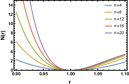
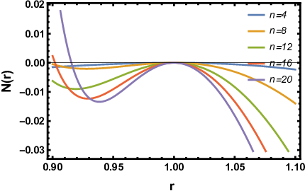
In Fig. (1), the plots for $N(r)$ are given for different values of $N^{\prime\prime}(r_{0})$ and dimension $n$ with a degenerate horizon at $r_{0}=1$. The analytical definition of $N(r)$ near the degenerate horizon is given by Eq. (32). Near the degenerate horizon, the space-time is written as in Eq. (33) in $n$-dimensions in different coordinate system. In this section, we study the anti-evaporation of $n$-dimensional black hole near the degenerate horizon. Here we implement perturbation analysis up to the linear order. It will be shown that $f(R)$ theory is relevant for the dynamical nature of the perturbation $\delta\phi$. Setting $f^{\prime\prime}(R_{0})=0$, one obtains $\delta\phi=0$, which indicates the constant horizon. Working with $f(R)$, the perturbation $\delta\phi$ becomes proportional to $\delta R$ and it gives a possibility of dynamical $\delta\phi$ . In simplifying constants we use the background equations. Maxwell field tensor is defined by $\nabla_{\mu}(F^{p-1}F^{\mu\nu})=0$ and is modified in $n$-dimensions.

References

- (1) P. Ivanov, “Nonlinear metric perturbations and production of primordial black holes,” Phys. Rev. D 57, 7145 (1998) [astro-ph/9708224].
- (2) J. S. Bullock and J. R. Primack, “Comments on nonGaussian density perturbations and the production of primordial black holes,” [astro-ph/9806301].
- (3) J. S. Bullock and J. R. Primack, “NonGaussian fluctuations and primordial black holes from inflation,” Phys. Rev. D 55, 7423 (1997) [astro-ph/9611106].
- (4) S. Hawking, “Gravitationally collapsed objects of very low mass,” Mon. Not. Roy. Astron. Soc. 152, 75 (1971).
- (5) B. J. Carr and S. W. Hawking, “Black holes in the early Universe,” Mon. Not. Roy. Astron. Soc. 168, 399 (1974).
- (6) O. K. Kalashnikov and M. Y. Khlopov, “On The Possibility Of Checking The Cosmology Of Asymptotically Free SU(5) Theory,” Phys. Lett. 127B, 407 (1983).
- (7) B. Carr, F. Kuhnel and M. Sandstad, “Primordial Black Holes as Dark Matter,” Phys. Rev. D 94, no. 8, 083504 (2016) [arXiv:1607.06077 [astro-ph.CO]].
- (8) P. Ivanov, P. Naselsky and I. Novikov, “Inflation and primordial black holes as dark matter,” Phys. Rev. D 50, 7173 (1994).
- (9) D. Blais, C. Kiefer and D. Polarski, “Can primordial black holes be a significant part of dark matter?,” Phys. Lett. B 535, 11 (2002) [astro-ph/0203520].
- (10) L. K. Chavda and A. L. Chavda, “Dark matter and stable bound states of primordial black holes,” Class. Quant. Grav. 19, 2927 (2002) [gr-qc/0308054].
- (11) S. W. Hawking, Commun. Math. Phys. 43, 199 (1975) Erratum: [Commun. Math. Phys. 46, 206 (1976)].
- (12) R. Bousso and S. W. Hawking, “(Anti)evaporation of Schwarzschild-de Sitter black holes,” Phys. Rev. D 57 (1998) 2436, [arXiv: 9709224 [hep-th]].
- (13) H. Nariai, Sci. Rep. Tohoku Univ. 34 (1950) 160.
- (14) H. Nariai, Sci. Rep. Tohoku Univ. 35 (1951) 62.
- (15) S. Nojiri and S. D. Odintsov, “Quantum evolution of Schwarzschild-de Sitter (Nariai) black holes,” Phys. Rev. D 59 (1999) 044026 [arXiv:9804033 [hep-th]].
- (16) M. Buric and V. Radovanovic, “Quantum corrections for anti-evaporating black hole,” Phys. Rev. D 63, 044020 (2001) [arXiv: 0007172 [hep-th]].
- (17) E. Elizalde, S. Nojiri and S. D. Odintsov, “Possible quantum instability of primordial black holes,” Phys. Rev. D 59, 061501 (1999) [hep-th/9901026].
- (18) A. A. Bytsenko, S. Nojiri and S. D. Odintsov, “Quantum generation of Schwarzschild-de Sitter (Nariai) black holes in effective Dilaton - Maxwell gravity,” Phys. Lett. B 443, 121 (1998) [hep-th/9808109].
- (19) J. C. Niemeyer and R. Bousso, “The Nonlinear evolution of de Sitter space instabilities,” Phys. Rev. D 62, 023503 (2000) [gr-qc/0004004].
- (20) S. Nojiri and S. D. Odintsov, “Effective action for conformal scalars and anti-evaporation of black holes,” Int. J. Mod. Phys. A 14, 1293 (1999) [hep-th/9802160].
- (21) S. Nojiri and S. D. Odintsov, “Quantum dilatonic gravity in (D = 2)-dimensions, (D = 4)-dimensions and (D = 5)-dimensions,” Int. J. Mod. Phys. A 16, 1015 (2001) [hep-th/0009202].
- (22) S. Nojiri and S. D. Odintsov, “Anti evaporation of Schwarzschild-de Sitter black holes in gravity,” Class. Quant. Grav. 30, 125003 (2013) [arXiv: 1301.2775 [hep-th]].
- (23) S. Nojiri and S. D. Odintsov, “Instabilities and anti-evaporation of Reissner-Nordström black holes in modified gravity,” Phys. Lett. B 735, 376 (2014) [arXiv:1405.2439 [gr-qc]].
- (24) Andrea Addazi “(Anti)evaporation of Dyonic Black Holes in string-inspired dilaton -gravity,” Int. J. Mod. Phys. A 32, no. 17, 1750102 (2017) [arXiv:1610.04094 [gr-qc]].
- (25) V. K. Oikonomou, “Reissner-Nordström Anti-de Sitter Black Holes in Mimetic Gravity,” Universe 2 (2016) no.2, 10, arXiv:1511.09117 [gr-qc].
- (26) Taishi Katsuragawa, Shin’ichi Nojiri “Stability and antievaporation of the Schwarzschild–de Sitter black holes in bigravity” Phys.Rev. D91 (2015) 084001, [arXiv: 1411.1610 [hep-th]].
- (27) D. V. Singh and N. K. Singh, “Anti-Evaporation of Bardeen de-Sitter Black Holes,” Annals Phys. 383, 600 (2017) [arXiv:1704.01831 [physics.gen-ph]].
- (28) A. Addazi, S. Nojiri and S. Odintsov, “Evaporation and anti-evaporation instability of a Schwarzschild-de Sitter braneworld: the case of five-dimensional F(R) gravity,” Phys. Rev. D 95, no. 12, 124020 (2017) [arXiv:1705.03265 [gr-qc]].
- (29) T. Kaluza, Sitzungsber. Preuss. Akad. Wiss. Berlin (Math. Phys. ) 1921, 966 (1921) [arXiv:1803.08616 [physics.hist-ph]].
- (30) O. Klein, Nature 118, 516 (1926).
- (31) T. Appelquist, A. Chodos and P. G. O. Freund, READING, USA: ADDISON-WESLEY (1987) 619 P. (FRONTIERS IN PHYSICS, 65).
- (32) M. J. Duff, B. E. W. Nilsson and C. N. Pope, Phys. Rept. 130, 1 (1986).
- (33) M. B. Green, J. H. Schwarz and E. Witten, “Superstring Theory Vol. 1: 25th Anniversary Edition,”(Cambridge University Press, Cambridge, England, 1987, doi:10.1017/CBO9781139248563
- (34) M. B. Green, J. H. Schwarz and E. Witten, “Superstring Theory Vol. 2: 25th Anniversary Edition,”(Cambridge University Press, Cambridge, England, 1987, doi:10.1017/CBO9781139248570
- (35) R. Emparan and H. S. Reall, “Black Holes in Higher Dimensions,” Living Rev. Rel. 11, 6 (2008) [arXiv:0801.3471 [hep-th]].
- (36) H. S. Reall, “Higher dimensional black holes,” Int. J. Mod. Phys. D 21, 1230001 (2012) [arXiv:1210.1402 [gr-qc]].
- (37) P. Kanti, “Black Holes at the LHC,” Lect. Notes Phys. 769, 387 (2009) [arXiv:0802.2218 [hep-th]].
- (38) A. Strominger and C. Vafa, “Microscopic origin of the Bekenstein-Hawking entropy,” Phys. Lett. B 379, 99 (1996) [hep-th/9601029].
- (39) R. C. Myers and M. J. Perry, “Black Holes in Higher Dimensional Space-Times,” Annals Phys. 172, 304 (1986).
- (40) D. Y. Xu, “Exact Solutions of Einstein and Einstein-maxwell Equations in Higher Dimensional Space-time,” Class. Quant. Grav. 5, 871 (1988).
- (41) J. T. Liu and W. A. Sabra, “Charged configurations in (A)dS spaces,” Nucl. Phys. B 679, 329 (2004) [hep-th/0307300].
- (42) S. G. Ghosh, “Nonstatic charged BTZ-like black holes in N+1 dimensions,” Int. J. Mod. Phys. D 21, 1250022 (2012) [arXiv:1109.3263 [gr-qc]].
- (43) S. H. Hendi, “Charged BTZ-like Black Holes in Higher Dimensions,” Eur. Phys. J. C 71, 1551 (2011) [arXiv:1007.2704 [gr-qc]].
- (44) S. G. Ghosh and D. Kothawala, “Radiating black hole solutions in arbitrary dimensions,” Gen. Rel. Grav. 40, 9 (2008) [arXiv:0801.4342 [gr-qc]].
- (45) A. Sheykhi, “Higher-dimensional charged black holes,” Phys. Rev. D 86, 024013 (2012) [arXiv:1209.2960 [hep-th]].
- (46) J. Matyjasek, P. Sadurski and D. Tryniecki, “Inside the degenerate horizons of regular black holes,” Phys. Rev. D 87, no. 12, 124025 (2013) [arXiv:1304.6347 [gr-qc]].
- (47) S. Fernando, “Bardeen-de Sitter black holes,” Int. J. Mod. Phys. D 26, no. 07, 1750071 (2017) [arXiv:1611.05337 [gr-qc]].