跳到论文正文
W Papers独立论文阅读器 arXiv:1811.11368 论文正文 计算阅读时间 · 0%
引用这篇论文根据当前论文元数据生成,正式投稿前建议核对。


License: arXiv.org perpetual non-exclusive license
arXiv:1811.11368v2 [stat.ML] 04 Feb 2021

First-order Newton-type Estimator for Distributed Estimation and Inference

Xi Chen   Weidong Liu   Yichen Zhang Note: Stern School of Business, New York University, Email: xichen3@stern.nyu.edu. Note: School of Mathematical Sciences, Shanghai Jiao Tong University, Email: weidongl@sjtu.edu.cn. Corresponding author. Note: Krannert School of Management, Purdue University, Email: zhang@purdue.edu.
Abstract

This paper studies distributed estimation and inference for a general statistical problem with a convex loss that could be non-differentiable. For the purpose of efficient computation, we restrict ourselves to stochastic first-order optimization, which enjoys low per-iteration complexity. To motivate the proposed method, we first investigate the theoretical properties of a straightforward Divide-and-Conquer Stochastic Gradient Descent (DC-SGD) approach. Our theory shows that there is a restriction on the number of machines and this restriction becomes more stringent when the dimension pp is large. To overcome this limitation, this paper proposes a new multi-round distributed estimation procedure that approximates the Newton step only using stochastic subgradient. The key component in our method is the proposal of a computationally efficient estimator of 𝚺−1​𝒘\bm{\Sigma}^{-1}\bm{w}, where 𝚺\bm{\Sigma} is the population Hessian matrix and 𝒘\bm{w} is any given vector. Instead of estimating 𝚺\bm{\Sigma} (or 𝚺−1\bm{\Sigma}^{-1}) that usually requires the second-order differentiability of the loss, the proposed First-Order Newton-type Estimator (FONE) directly estimates the vector of interest 𝚺−1​𝒘\bm{\Sigma}^{-1}\bm{w} as a whole and is applicable to non-differentiable losses. Our estimator also facilitates the inference for the empirical risk minimizer. It turns out that the key term in the limiting covariance has the form of 𝚺−1​𝒘\bm{\Sigma}^{-1}\bm{w}, which can be estimated by FONE.

1 Introduction

The development of modern technology has enabled data collection of unprecedented size, which poses new challenges to many statistical estimation and inference problems. First, given NN samples with a very large NN, a standard machine might not have enough memory to load the entire dataset all at once. Second, a deterministic optimization approach is computationally expensive. To address the storage and computation issues, distributed computing methods, originated from computer science literature, has been recently introduced into statistics. A general distributed computing scheme partitions the entire dataset into LL parts, and then loads each part into the memory to compute a local estimator. The final estimator will be obtained via some communication and aggregation among local estimators.

To further accelerate the computation, we consider stochastic first-order methods (e.g., stochastic gradient/subgradient descent (SGD)), which have been widely adopted in practice. There are a few significant advantages of SGD. First, as a first-order method, it only requires the subgradient information. As compared to second-order Newton-type approaches, it is not only computationally efficient and more scalable but also has a wider range of applications to problems where the empirical Hessian matrix does not exist (e.g., when the loss is non-smooth such as quantile regression). Second, a stochastic approach is usually more efficient than its deterministic counterpart. Although SGD has been widely studied in machine learning and optimization, using SGD for the purpose of statistical inference has not been sufficiently explored.

This paper studies a general statistical estimation and inference problem under the distributed computing setup. As we mentioned, to achieve an efficient computation, we restrict ourselves to the use of only stochastic subgradient information. In particular, consider a general statistical estimation problem in the following risk minimization form,

𝜽∗=arg​min𝜽∈ℝp⁡F⁡(𝜽):=𝔼𝝃∼Π​f​(𝜽,𝝃),\displaystyle\bm{\theta}^{*}=\mathop{\rm arg\min}_{\bm{\theta}\in\mathbb{R}^{p}}F(\bm{\theta}):=\mathbb{E}_{\bm{\xi}\sim\Pi}f(\bm{\theta},\bm{\xi}), (1)

where f⁡(⋅,𝝃):ℝp→ℝf(\cdot,\bm{\xi}):\mathbb{R}^{p}\rightarrow\mathbb{R} is a convex loss function that can be non-differentiable (e.g., in quantile regression), and 𝝃\bm{\xi} denotes the random sample from a probability distribution Π\Pi (e.g., 𝝃=(Y,𝑿)\bm{\xi}=(Y,\bm{X}) in a regression setup). Our goal is to estimate 𝜽∗∈ℝp\bm{\theta}^{*}\in\mathbb{R}^{p} under the diverging dimension case, where the dimensionality pp is allowed to go to infinity as the sample size grows (but pp grows at a slower rate than the sample size). This regime is more challenging than the fixed pp case. On the other hand, since this work does not make any sparsity assumption, the high dimensional setting where pp could be potentially larger than the sample size is beyond our scope. For the ease of illustration, we will use two motivating examples throughout the paper: (1) logistic regression with a differentiable loss, and (2) quantile regression with a non-differentiable loss.

Given nn i.i.d. samples11 1 With a slight abuse of notation, we use nn to denote either the sample size in non-distributed settings or the local sample size of a single machine in distributed settings. {𝝃i}i=1n\{\bm{\xi}_{i}\}_{i=1}^{n}, a traditional non-distributed approach for estimating 𝜽∗\bm{\theta}^{*} is to minimize the empirical risk via a deterministic optimization:

𝜽^=arg​min𝜽∈ℝp⁡1n​∑i=1nf⁡(𝜽,𝝃i).\widehat{\bm{\theta}}=\mathop{\rm arg\min}_{\bm{\theta}\in\mathbb{R}^{p}}\frac{1}{n}\sum_{i=1}^{n}f(\bm{\theta},\bm{\xi}_{i}). (2)

Moreover, let g⁡(𝜽,𝝃)g(\bm{\theta},\bm{\xi}) be the gradient (when f⁡(𝜽,𝝃)f(\bm{\theta},\bm{\xi}) is differentiable) or a subgradient (when f⁡(𝜽,𝝃)f(\bm{\theta},\bm{\xi}) is non-differentiable) of f⁡(𝜽,𝝃)f(\bm{\theta},\bm{\xi}) at 𝜽\bm{\theta}. In terms of statistical inference, for many popular statistical models, the empirical risk minimizer (ERM) 𝜽^\widehat{\bm{\theta}} has an asymptotic normal distribution. That is, under some regularity conditions, for a fixed unit length vector 𝒘∈ℝp\bm{w}\in\mathbb{R}^{p}, as n,p→∞n,p\rightarrow\infty,

n​𝒘′​(𝜽^−𝜽∗)𝒘′​𝚺−1​𝑨​𝚺−1​𝒘→𝒩⁡(0,1),\frac{\sqrt{n}\bm{w}^{\prime}(\widehat{\bm{\theta}}-\bm{\theta}^{*})}{\sqrt{\bm{w}^{\prime}\bm{\Sigma}^{-1}\bm{A}\bm{\Sigma}^{-1}\bm{w}}}\rightarrow\mathcal{N}(0,1), (3)

where

𝚺:=∇𝜽𝔼​g​(𝜽,𝝃)|𝜽=𝜽∗𝑨=Cov​(g⁡(𝜽∗,𝝃))=𝔼⁡[g⁡(𝜽∗,𝝃)​g​(𝜽∗,𝝃)′].\bm{\Sigma}:=\nabla_{\bm{\theta}}\mathbb{E}g(\bm{\theta},\bm{\xi})|_{\bm{\theta}=\bm{\theta}^{*}}\quad\bm{A}=\textsf{Cov}(g(\bm{\theta}^{*},\bm{\xi}))=\mathbb{E}\left[g(\bm{\theta}^{*},\bm{\xi})g(\bm{\theta}^{*},\bm{\xi})^{\prime}\right]. (4)

Under this framework, the main goal of our paper is twofold:

  1. 1.

    Distributed estimation: Develop a distributed stochastic first-order method for estimating 𝜽∗\bm{\theta}^{*} in the case of diverging pp, with the aim to achieve the best possible convergence rate (i.e., the rate of the pooled ERM estimator 𝜽^\widehat{\bm{\theta}}). The method should be applicable to non-differentiable loss f⁡(𝜽,𝝃)f(\bm{\theta},\bm{\xi}) and only requires the local strong convexity of F⁡(𝜽)F(\bm{\theta}) at 𝜽=𝜽∗\bm{\theta}=\bm{\theta}^{*} (instead of the strong convexity of F⁡(𝜽)F(\bm{\theta}) for any 𝜽\bm{\theta}).

  2. 2.

    Distributed inference: Based on (3), develop a consistent estimator of the limiting variance 𝒘′​𝚺−1​𝑨​𝚺−1​𝒘\bm{w}^{\prime}\bm{\Sigma}^{-1}\bm{A}\bm{\Sigma}^{-1}\bm{w} to facilitate the inference.

Let us first focus on the distributed estimation problem. We will first investigate the theoretical proprieties of a straightforward method that combines the stochastic subgradient descent (SGD) and divide-and-conquer (DC) scheme and discuss the theoretical limitation of this method. To overcome the theoretical limitation, we propose a new method called the distributed First-Order Newton-type Estimator (FONE), where the key idea is to approximate the Newton step only using stochastic subgradient information in a distributed setting.

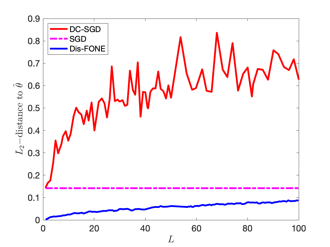
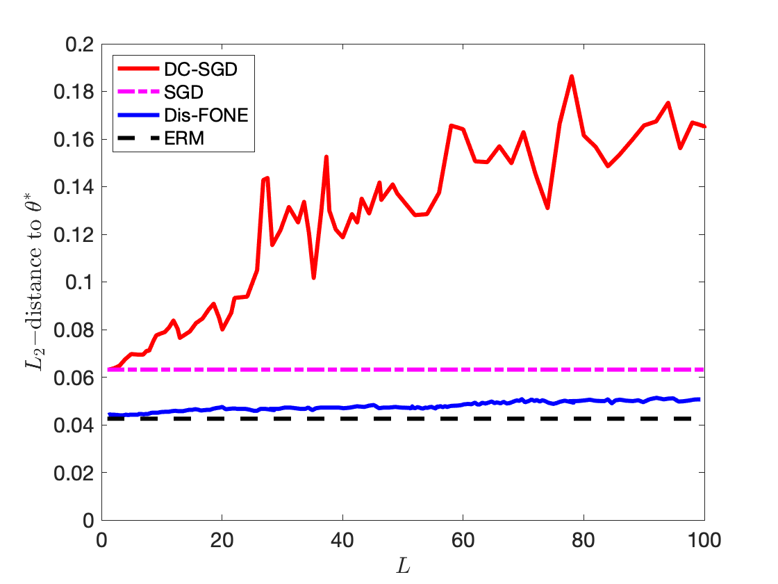
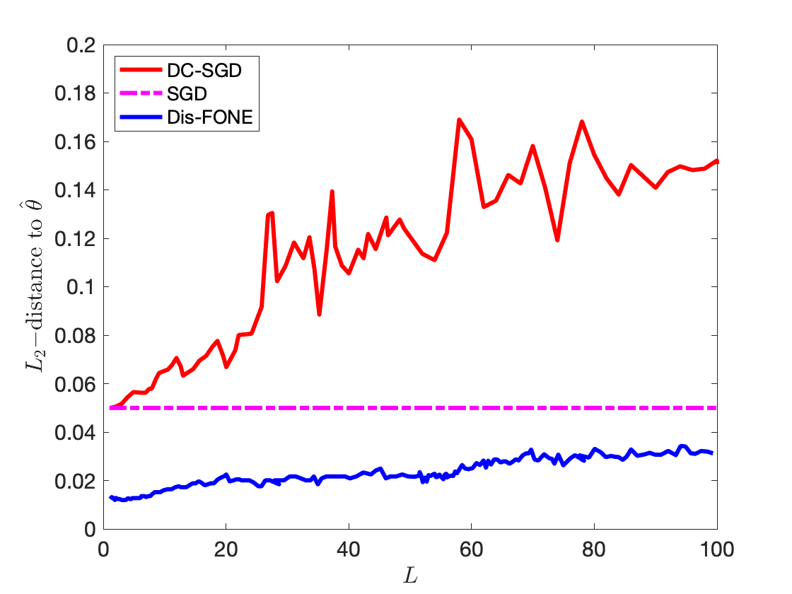
In a distributed setting, the divide-and-conquer (DC) strategy has been recently adopted in many statistical estimation problems (see, e.g., Li et al. 2013; Chen and Xie 2014; Huang and Huo 2019; Zhang et al. 2015; Battey et al. 2018; Zhao et al. 2016; Shi et al. 2018; Banerjee et al. 2019; Volgushev et al. 2019; Fan et al. 2019. A standard DC approach estimates a local estimator for each local machine. and then aggregates the local estimators to obtain the final estimator. Combining the idea of DC with the mini-batch SGD naturally leads to a divide-and-conquer SGD (DC-SGD) approach, where we run SGD on each local machine and then aggregate the obtained solutions by an averaging operation. In fact, DC-SGD is not the main focus/contribution of this paper. It has been an existing popular distributed algorithm in practice for a long time. Nevertheless, the theoretical property of DC-SGD with mini-batch in the diverging dimension case has not been fully understood yet. We first establish the theoretical properties of DC-SGD and explain its limitations, which better motivates our distributed estimator (see below). For DC-SGD to achieve the optimal convergence rate, the number of machines LL has to be O⁡(N/p)O(\sqrt{N/p}) (see Section 3.1), where NN is the total number of samples across LL machines. The condition could be restrictive when the number of machines is large but each local machine has a limited storage (e.g., in a large-scale sensor network). Moreover, as compared to the standard condition L=O⁡(N)L=O(\sqrt{N}) in a fixed pp setting, the condition L=O⁡(N/p)L=O(\sqrt{N/p}) becomes more stringent when pp diverges. In fact, this constraint is not only for the case of DC-SGD. Since the averaging only reduces the variance but not the bias term, all the results for the standard DC approach in the literature inevitably involve a constraint on the number of machines, which aims to make the variance the dominating term.

To relax this condition on LL and further improve the performance of DC-SGD, this paper proposes a new approach called distributed first-order Newton-type estimator, which successively refines the estimator by multi-round aggregations. The starting point of our approach is the Newton-type method based on a consistent initial estimator 𝜽^0\widehat{\bm{\theta}}_{0}:

𝜽~=𝜽^0−𝚺−1​(1n​∑i=1ng⁡(𝜽^0,𝝃i)),\widetilde{\bm{\theta}}=\widehat{\bm{\theta}}_{0}-\bm{\Sigma}^{-1}\left(\frac{1}{n}\sum_{i=1}^{n}g(\widehat{\bm{\theta}}_{0},\bm{\xi}_{i})\right), (5)

where 𝚺\bm{\Sigma} is the population Hessian matrix and (1n​∑i=1ng⁡(𝜽^0,𝝃i))\left(\frac{1}{n}\sum_{i=1}^{n}g(\widehat{\bm{\theta}}_{0},\bm{\xi}_{i})\right) is the subgradient vector. However, the estimation of 𝚺\bm{\Sigma} is not easy when ff is non-differentiable and the empirical Hessian matrix does not exist.

To address this issue, our key idea is that instead of estimating 𝚺\bm{\Sigma} and computing its inverse, we propose an estimator of 𝚺−1​𝒘∈ℝp\bm{\Sigma}^{-1}\bm{w}\in\mathbb{R}^{p} for any given vector 𝒘∈ℝp\bm{w}\in\mathbb{R}^{p}, which solves (5) as a special case (with 𝒘=1n​∑i=1ng⁡(𝜽^0,𝝃i)\bm{w}=\frac{1}{n}\sum_{i=1}^{n}g(\widehat{\bm{\theta}}_{0},\bm{\xi}_{i})). In fact, the estimator of 𝚺−1​𝒘\bm{\Sigma}^{-1}\bm{w} kills two birds with one stone: it not only constructs a Newton-type estimator of 𝜽∗\bm{\theta}^{*} but also provides an estimator for the asymptotic variance in (3), which facilitates the inference. In particular, the proposed FONE estimator of 𝚺−1​𝒘\bm{\Sigma}^{-1}\bm{w} is an iterative procedure that only utilizes the mini-batches of subgradient to approximate the Newton step.

It is also worthwhile noting that our method extends the recent work by Jordan et al. 2019 and Wang and Zhang 2017, which approximates the Newton step by using local Hessian matrix computed on a single machine. However, to compute the local Hessian matrix, their method requires the second-order differentiability on the loss function and thus is not applicable to problems such as quantile regression. In contrast, our approach approximates the Newton step via stochastic subgradient and thus can handle the non-differentiability in the loss function. We also note that the idea of approximating Newton step has been applied to specific statistical learning problems, such as SVM (Wang et al. 2019), quantile regression (Chen et al. 2019; Chen et al. 2020), and PCA (Chen et al. 2021). This paper provides a general framework for both smooth and non-smooth loss functions. Moreover, our method subsumes a recently developed stochastic first-order approach—stochastic variance reduced gradient (SVRG, see e.g., Johnson and Zhang 2013; Lee et al. 2017; Wang and Zhang 2017; Li et al. 2018 and references therein) as a special case. While SVRG requires 𝒘\bm{w} to be the averaged gradient and its theory only applies to strongly convex smooth loss functions, we allow a general 𝒘\bm{w} vector and non-smooth losses.

Based on FONE, we further develop a multi-round distributed version of FONE which successively refines the estimator and does not impose any strict condition on the number of machines LL. Theoretically, we show that for a smooth loss, when the number of rounds KK exceeds a constant threshold K0K_{0}, the obtained distributed FONE 𝜽^dis,K\widehat{\bm{\theta}}_{\mathrm{dis},K} achieves the optimal convergence rate. For a non-smooth loss, such as quantile regression, our convergence rate only depends on the sample size of one local machine with the largest sub-sample size. This condition is weaker than the case of DC-SGD since the bottleneck in the convergence of DC-SGD is the local machine with the smallest sub-sample size.

We further apply the developed FONE to obtain a consistent estimator of the asymptotic variance in (3) for the purpose of inference. Note that the term 𝑨\bm{A} can be easily estimated via replacing the expectation by its sample version. Instead of estimating 𝚺−1\bm{\Sigma}^{-1} in (3), our method directly estimates 𝚺−1​𝒘\bm{\Sigma}^{-1}\bm{w} for any fixed unit length vector 𝒘\bm{w} (please see Section 4 for more details).

The remainder of the paper is organized as follows: Section 2.1 describes the mini-batch SGD algorithm with diverging dimension and the DC-SGD estimator. We further propose FONE and distributed FONE in Section 2.2. Section 3 presents the theoretical results. Section 4 discusses the application of FONE to the inference problem. In Section 5, we demonstrate the performance of the proposed estimators by simulation experiments and real data analysis, followed by conclusions in Section 6. Some additional theoretical results, technical proofs and additional experimental results are provided in Appendix.

In this paper, we denote the Euclidean norm for a vector 𝒙∈ℝp\bm{x}\in\mathbb{R}^{p} by ‖𝒙‖2\|\bm{x}\|_{2}, and we denote the spectral norm for a matrix 𝑿\bm{X} by ‖𝑿‖\|\bm{X}\|. In addition, since the distributed estimation and inference usually involve quite a few notations, we briefly summarize them here. We use NN, LL, n=N/Ln=N/L, and mm to denote the total number of samples, the number of machines (or the number of data partitions), the sample size on each local machine (when evenly distributed), and the batch size for mini-batch SGD, respectively. When we discuss a problem in the classical single machine setting, we will also use nn to denote the sample size. We will use 𝜽∗\bm{\theta}^{*}, 𝜽^\widehat{\bm{\theta}}, and 𝜽^0\widehat{\bm{\theta}}_{0} to denote the minimizer of the popular risk, the ERM, and the initial estimator, respectively. The random sample will be denoted by 𝝃\bm{\xi} and in a regression setting 𝝃=(Y,𝑿)\bm{\xi}=(Y,\bm{X}).

2 Methodology

In this section, we first introduce the standard DC-SGD algorithm. The main purpose of introducing this DC-SGD algorithm is to better motivate the proposed FONE and its distributed version.

2.1 Divide-and-conquer SGD (DC-SGD) algorithm

Before we introduce our DC-SGD algorithm, we first present the mini-batch SGD algorithm for solving the stochastic optimization in (1) on a single machine with total nn samples. In particular, we consider the setting when the dimension p→∞p\rightarrow\infty but at a slower rate than nn, i.e., p≤nκp\leq n^{\kappa} for some κ∈(0,1)\kappa\in(0,1). Given nn i.i.d. samples {𝝃1,…,𝝃n}\{\bm{\xi}_{1},\ldots,\bm{\xi}_{n}\}, we partition the index set {1,…,n}\{1,\ldots,n\} into ss disjoint mini-batches H1,…,HsH_{1},...,H_{s}, where each mini-batch has the size |Hi|=m|H_{i}|=m (for i=1,2,…,si=1,2,\dots,s), and s=n/ms=n/m is the number of mini-batches. The mini-batch SGD algorithm starts from a consistent initial estimator 𝜽^0\widehat{\bm{\theta}}_{0} of 𝜽∗\bm{\theta}^{*}. Let 𝒛0=𝜽^0\bm{z}_{0}=\widehat{\bm{\theta}}_{0}. The mini-batch SGD iteratively updates 𝒛i\bm{z}_{i} from 𝒛i−1\bm{z}_{i-1} as follows and outputs 𝜽^SGD=𝒛s\widehat{\bm{\theta}}_{\mathrm{SGD}}=\bm{z}_{s} as its final estimator,

𝒛i=𝒛i−1−rim∑j∈Hig(𝒛i−1,𝝃j),fori=1,2,…,s,\displaystyle\bm{z}_{i}=\bm{z}_{i-1}-\frac{r_{i}}{m}\sum_{j\in H_{i}}g(\bm{z}_{i-1},\bm{\xi}_{j}),\quad\text{for}\;\;\;i=1,2,\ldots,s, (6)

where we set the step-size ri=c0/max⁡(iα,p)r_{i}=c_{0}/\max(i^{\alpha},p) for some 0<α≤10<\alpha\leq 1 and c0c_{0} is a positive constant. It is worthwhile that a typical choice of rir_{i} in the literature is ri=c0⋅i−αr_{i}=c_{0}\cdot{i}^{-\alpha} (Polyak and Juditsky 1992; Chen et al. 2020). Since we are considering a diverging pp case, our step-size incorporates the dimension pp. As one can see, this mini-batch SGD algorithm only uses one pass of the data and enjoys a low per-iteration complexity.

We provide two examples on logistic regression and quantile regression to illustrate the subgradient function g⁡(𝜽,𝝃)g(\bm{\theta},\bm{\xi}) in our mini-batch SGD and will refer to these examples throughout the paper.

Example 2.1 (Logistic regression).

Consider a logistic regression model with the response Y∈{−1,1}Y\in\{-1,1\}, where

ℙ⁡(Y=1|𝑿)=1−ℙ⁡(Y=−1|𝑿)=11+exp⁡(−𝑿′​𝜽∗),\displaystyle\mathbb{P}(Y=1|\bm{X})=1-\mathbb{P}(Y=-1|\bm{X})=\frac{1}{1+\mathrm{exp}(-\bm{X}^{\prime}\bm{\theta}^{*})},

and 𝛉∗∈ℝp\bm{\theta}^{*}\in\mathbb{R}^{p} is the true model parameter. Define 𝛏=(Y,𝐗)\bm{\xi}=(Y,\bm{X}). We have the smooth loss function f⁡(𝛉,𝛏)=log⁡(1+exp⁡(−Y​𝐗′​𝛉))f(\bm{\theta},\bm{\xi})=\log(1+\exp(-Y\bm{X}^{\prime}\bm{\theta})) and its gradient g⁡(𝛉,𝛏)=−Y​𝐗​(1+exp⁡(Y​𝐗′​𝛉))−1g(\bm{\theta},\bm{\xi})=-Y\bm{X}\big(1+\exp(Y\bm{X}^{\prime}\bm{\theta})\big)^{-1}.

Example 2.2 (Quantile regression).

Consider a quantile regression model Y=𝐗′​𝛉∗+ϵ,Y=\bm{X}^{\prime}\bm{\theta}^{*}+\epsilon, where we assume that 𝐗=(1,X1,…,Xp−1)′\bm{X}=(1,X_{1},...,X_{p-1})^{\prime} and ℙ⁡(ϵ≤0|𝐗)=τ\mathbb{P}(\epsilon\leq 0|\bm{X})=\tau is the so-called quantile level. Define 𝛏=(Y,𝐗)\bm{\xi}=(Y,\bm{X}). We have the non-smooth quantile loss function f⁡(𝛉,𝛏)=ℓτ​(Y−𝐗′​𝛉)f(\bm{\theta},\bm{\xi})=\ell_{\tau}(Y-\bm{X}^{\prime}\bm{\theta}) and ℓτ(x)=x(τ−I{x≤0})\ell_{\tau}(x)=x(\tau-I\{x\leq 0\}). A subgradient of the quantile loss is given by g(𝛉,𝛏)=𝐗(I{Y≤𝐗′𝛉}−τ)g(\bm{\theta},\bm{\xi})=\bm{X}(I\{Y\leq\bm{X}^{\prime}\bm{\theta}\}-\tau).

The bias and L2L_{2}-estimation error of the mini-batch SGD will be provided in Theorem B.1 (see Appendix B). In particular, in the diverging dimension setting, it is necessary to have a consistent initial estimator to guarantee the consistency of obtained solution from the mini-batch SGD (see Proposition B.2 in Appendix).

Given the mini-batch SGD, we are ready to introduce the divide-and-conquer SGD (DC-SGD). For the ease of illustration, suppose that the entire sample with the size NN is evenly distributed on LL machines (or split into LL parts) with the sub-sample size n=N/Ln=N/L on each local machine. For the ease of presentation, we assume that N/LN/L is a positive integer. On each machine k=1,2,…,Lk=1,2,\dots,L, we run the mini-batch SGD with the batch size mm in (6). Let ℋk\mathcal{H}_{k} be the indices of the data points on the kk-th machine, which is further split into ss mini-batches {Hk,i,i=1,2,…,s}\{H_{k,i},i=1,2,\dots,s\} with |Hk,i|=m|H_{k,i}|=m and s=n/ms=n/m. On the kk-th machine, we run our mini-batch SGD in (6) and obtain the local estimator 𝜽^SGD(k)\widehat{\bm{\theta}}_{\mathrm{SGD}}^{(k)}. The final estimator is aggregated by averaging the local estimators from LL machines, i.e.,

𝜽^DC=1L​∑k=1L𝜽^SGD(k).\displaystyle\widehat{\bm{\theta}}_{\mathrm{DC}}=\dfrac{1}{L}\sum\limits_{k=1}^{L}\widehat{\bm{\theta}}_{\mathrm{SGD}}^{(k)}. (7)

Note that the DC-SGD algorithm only involves one round of aggregation. The details of the DC-SGD are presented in Algorithm 1.

Algorithm 1 DC-SGD algorithm

Input: The initial estimator 𝜽^0∈ℝp\widehat{\bm{\theta}}_{0}\in\mathbb{R}^{p}, the step-size sequence ri=c0/max⁡(iα,p)r_{i}=c_{0}/\max(i^{\alpha},p) for some 0<α≤10<\alpha\leq 1, the mini-batch size mm.

1:  Distribute the initial estimator 𝜽^0\widehat{\bm{\theta}}_{0} to each local machine k=1,2,…,Lk=1,2,\dots,L.
2:  for each local machine k=1,2,…,Lk=1,2,\dots,L do
3:   Set the starting point 𝒛0(k)=𝜽^0\bm{z}_{0}^{(k)}=\widehat{\bm{\theta}}_{0}.
4:   for each iteration i=1,…,si=1,\dots,s do
5:    Update
𝒛i(k)=𝒛i−1(k)−rim​∑j∈Hk,ig⁡(𝒛i−1(k),𝝃j),\bm{z}_{i}^{(k)}=\bm{z}_{i-1}^{(k)}-\frac{r_{i}}{m}\sum_{j\in H_{k,i}}g(\bm{z}_{i-1}^{(k)},\bm{\xi}_{j}),
6:   end for
7:   Set 𝜽^SGD(k)=𝒛s(k)\widehat{\bm{\theta}}_{\mathrm{SGD}}^{(k)}=\bm{z}_{s}^{(k)} as the local SGD estimator on the machine kk.
8:  end for
9:  Aggregate the local estimators 𝜽^SGD(k)\widehat{\bm{\theta}}_{\mathrm{SGD}}^{(k)} by averaging and compute the final estimator:
𝜽^DC=1L​∑k=1L𝜽^SGD(k).\widehat{\bm{\theta}}_{\mathrm{DC}}=\dfrac{1}{L}\sum\limits_{k=1}^{L}\widehat{\bm{\theta}}_{\mathrm{SGD}}^{(k)}.
10:  Output: 𝜽^DC\widehat{\bm{\theta}}_{\mathrm{DC}}.

In Theorem 3.1, we establish the convergence rate of the DC-SGD in terms of the dimension pp, the number of machines LL, the total sample size NN and the mini-batch size mm. Moreover, we show that for the DC-SGD to achieve the same rate as the mini-batch SGD running on the entire dataset, it requires a condition on the number of machines LL. This condition is essential because the averaging scheme in a divide-and-conquer approach only reduces the variance but not the bias term.

2.2 First-Order Newton-type Estimator (FONE)

Algorithm 2 First-Order Newton-type Estimator (FONE) of 𝚺−1​𝒂\bm{\Sigma}^{-1}\bm{a}

Input: Dataset {𝝃1,𝝃2,…,𝝃n}\{\bm{\xi}_{1},\bm{\xi}_{2},\dots,\bm{\xi}_{n}\}, the initial estimator 𝜽^0\widehat{\bm{\theta}}_{0}, step-size η\eta, the batch-size mm, and a given vector 𝒂∈ℝp\bm{a}\in\mathbb{R}^{p}.

1:  Set 𝒛0=𝜽^0\bm{z}_{0}=\widehat{\bm{\theta}}_{0}.
2:  for each t=1,2,…,Tt=1,2,\dots,T do
3:   Choose BtB_{t} to be mm distinct elements uniformly from {1,2,…,n}\{1,2,...,n\}.
4:   Calculate
gBt​(𝒛t−1)=1m​∑i∈Btg⁡(𝒛t−1,𝝃i),gBt​(𝒛0)=1m​∑i∈Btg⁡(𝒛0,𝝃i).g_{B_{t}}(\bm{z}_{t-1})=\frac{1}{m}\sum_{i\in B_{t}}g(\bm{z}_{t-1},\bm{\xi}_{i}),\qquad g_{B_{t}}(\bm{z}_{0})=\frac{1}{m}\sum_{i\in B_{t}}g(\bm{z}_{0},\bm{\xi}_{i}).
5:   Update
𝒛t=𝒛t−1−η⁡{gBt​(𝒛t−1)−gBt​(𝒛0)+𝒂}.\bm{z}_{t}=\bm{z}_{t-1}-\eta\{g_{B_{t}}(\bm{z}_{t-1})-g_{B_{t}}(\bm{z}_{0})+\bm{a}\}.
6:  end for
7:  Output:
𝜽^FONE=𝜽^0−𝒛T.\widehat{\bm{\theta}}_{\mathrm{FONE}}=\widehat{\bm{\theta}}_{0}-\bm{z}_{T}. (8)

To relax the condition on the number of machines LL, one idea is to perform a Newton-type step in (5). However, as we have pointed out, the estimation of 𝚺\bm{\Sigma} requires the second-order differentiability of the loss function. Moreover, a typical Newton method successively refines the estimator of 𝚺\bm{\Sigma} based on the current estimate of 𝜽∗\bm{\theta}^{*} and thus requires the computation of matrix inversion in (5) for multiple iterations, which could be computationally expensive when pp is large.

In this section, we propose a new First-Order Newton-type Estimator that directly estimates 𝚺−1​𝒂\bm{\Sigma}^{-1}\bm{a} (for any given vector 𝒂\bm{a}) only using the stochastic first-order information. Then for a given initial estimator 𝜽^0\widehat{\bm{\theta}}_{0}, we can perform the Newton-type step in (5) as

𝜽~=𝜽^0−𝚺−1​𝒂^,𝒂=(1n​∑i=1ng⁡(𝜽^0,𝝃i)),\widetilde{\bm{\theta}}=\widehat{\bm{\theta}}_{0}-\widehat{\bm{\Sigma}^{-1}\bm{a}},\qquad\bm{a}=\left(\frac{1}{n}\sum_{i=1}^{n}g(\widehat{\bm{\theta}}_{0},\bm{\xi}_{i})\right), (9)

where 𝚺−1​𝒂^\widehat{\bm{\Sigma}^{-1}\bm{a}} is our estimator of 𝚺−1​𝒂\bm{\Sigma}^{-1}\bm{a}.

To estimate 𝚺−1​𝒂\bm{\Sigma}^{-1}\bm{a}, we note that 𝚺−1​𝒂=∑i=0∞(I−η​𝚺)i​η​𝒂\bm{\Sigma}^{-1}\bm{a}=\sum\limits_{i=0}^{\infty}(I-\eta\bm{\Sigma})^{i}\eta\bm{a} for small enough η\eta such that ‖η​𝚺‖<1\|\eta\bm{\Sigma}\|<1. Then we can use the following iterative procedure {𝒛~t}\{\widetilde{\bm{z}}_{t}\} to approximate 𝚺−1​𝒂\bm{\Sigma}^{-1}\bm{a}:

𝒛~t=𝒛~t−1−η⁡(𝚺​𝒛~t−1−𝒂), 1≤t≤T,\displaystyle\widetilde{\bm{z}}_{t}=\widetilde{\bm{z}}_{t-1}-\eta(\bm{\Sigma}\widetilde{\bm{z}}_{t-1}-\bm{a}),\ 1\leq t\leq T, (10)

where η\eta here can be viewed as a constant step-size. To see that (10) leads to an approximation of 𝚺−1​𝒂\bm{\Sigma}^{-1}\bm{a}, when TT is large enough, we have

𝒛~T\displaystyle\widetilde{\bm{z}}_{T} =\displaystyle= 𝒛~T−1−η⁡(𝚺​𝒛~T−1−𝒂)=(I−η​𝚺)​𝒛~T−1+η​𝒂\displaystyle\widetilde{\bm{z}}_{T-1}-\eta(\bm{\Sigma}\widetilde{\bm{z}}_{T-1}-\bm{a})=(I-\eta\bm{\Sigma})\widetilde{\bm{z}}_{T-1}+\eta\bm{a}
=\displaystyle= (I−η​𝚺)2​𝒛~T−2+(I−η​𝚺)​η​𝒂+η​𝒂\displaystyle(I-\eta\bm{\Sigma})^{2}\widetilde{\bm{z}}_{T-2}+(I-\eta\bm{\Sigma})\eta\bm{a}+\eta\bm{a}
=\displaystyle= (I−η​𝚺)T−1​𝒛~1+∑i=0T−2(I−η​𝚺)i​η​𝒂≈𝚺−1​𝒂.\displaystyle(I-\eta\bm{\Sigma})^{T-1}\widetilde{\bm{z}}_{1}+\sum_{i=0}^{T-2}(I-\eta\bm{\Sigma})^{i}\eta\bm{a}\approx\bm{\Sigma}^{-1}\bm{a}.

As the iterate 𝒛~t\widetilde{\bm{z}}_{t} approximates 𝚺−1​𝒂\bm{\Sigma}^{-1}\bm{a}, let us define 𝒛t=𝜽^0−𝒛~t\bm{z}_{t}=\widehat{\bm{\theta}}_{0}-\widetilde{\bm{z}}_{t}, which is the quantity of interest (see the left-hand side of the Newton-type step in (9)). To avoid estimating 𝚺\bm{\Sigma} in the recursive update in (10), we adopt the following first-order approximation:

−𝚺​𝒛~t−1=𝚺⁡(𝒛t−1−𝜽^0)≈gBt​(𝒛t−1)−gBt​(𝜽^0),-\bm{\Sigma}\widetilde{\bm{z}}_{t-1}=\bm{\Sigma}(\bm{z}_{t-1}-\widehat{\bm{\theta}}_{0})\approx g_{B_{t}}(\bm{z}_{t-1})-g_{B_{t}}(\widehat{\bm{\theta}}_{0}), (11)

where gBt​(𝜽)=1m​∑i∈Btg⁡(𝜽,𝝃i)g_{B_{t}}(\bm{\theta})=\frac{1}{m}\sum_{i\in B_{t}}g(\bm{\theta},\bm{\xi}_{i}) is the averaged stochastic subgradient over a subset of the data indexed by Bt⊆{1,2,…,n}B_{t}\subseteq\{1,2,\ldots,n\}. Here BtB_{t} is randomly chosen from {1,…,n}\{1,\ldots,n\} with replacement for every iteration.

Given (11), we construct our FONE of 𝜽^0−𝚺−1​𝒂\widehat{\bm{\theta}}_{0}-\bm{\Sigma}^{-1}\bm{a} by the following recursive update from t=1,2,…,Tt=1,2,\dots,T:

𝒛t=𝒛t−1−η⁡{gBt​(𝒛t−1)−gBt​(𝜽^0)+𝒂},𝒛0=𝜽^0.\displaystyle\bm{z}_{t}=\bm{z}_{t-1}-\eta\{g_{B_{t}}(\bm{z}_{t-1})-g_{B_{t}}(\widehat{\bm{\theta}}_{0})+\bm{a}\},\quad\bm{z}_{0}=\widehat{\bm{\theta}}_{0}. (12)

The obtained 𝒛T\bm{z}_{T}, as an estimator of 𝜽^0−𝚺−1​𝒂\widehat{\bm{\theta}}_{0}-\bm{\Sigma}^{-1}\bm{a} can be directly used in the Newton-type step in (9). The choices of the input parameters and the convergence rate of our FONE will be proved in Propositions 3.2 and 3.4. Also note that for constructing the estimator of 𝚺−1​𝒂\bm{\Sigma}^{-1}\bm{a}, we can simply use 𝜽^0−𝒛T\widehat{\bm{\theta}}_{0}-\bm{z}_{T} and the procedure is summarized in Algorithm 2.

Algorithm 3 Distributed FONE for Estimating 𝜽∗\bm{\theta}^{*} in (1)

Input: The total sample size NN, the entire data {𝝃1,𝝃2,…,𝝃N}\{\bm{\xi}_{1},\bm{\xi}_{2},\dots,\bm{\xi}_{N}\} is distributed into LL machines/parts {ℋk}\{\mathcal{H}_{k}\} for k=1,2​…,Lk=1,2\ldots,L with |ℋk|=nk|\mathcal{H}_{k}|=n_{k}. Initial estimator 𝜽^0∈ℝp\widehat{\bm{\theta}}_{0}\in\mathbb{R}^{p}, the batch size mm, step-size η\eta. Number of rounds KK.

1:  for each round j=1,2,…,Kj=1,2,\dots,K do
2:   for each local machine k=1,2,…,Lk=1,2,\dots,L do
3:    Calculate ∑i∈ℋkg⁡(𝜽^j−1,𝝃i).\sum\limits_{i\in\mathcal{H}_{k}}g(\widehat{\bm{\theta}}_{j-1},\bm{\xi}_{i}).
4:   end for
5:   Collect ∑i∈ℋkg⁡(𝜽^j−1,𝝃i)\sum\limits_{i\in\mathcal{H}_{k}}g(\widehat{\bm{\theta}}_{j-1},\bm{\xi}_{i}) from each local machine to compute their average:
𝒂=1N​∑k=1L∑i∈ℋkg⁡(𝜽^j−1,𝝃i)=1N​∑i=1Ng⁡(𝜽^j−1,𝝃i).\bm{a}=\frac{1}{N}\sum\limits_{k=1}^{L}\sum\limits_{i\in\mathcal{H}_{k}}g(\widehat{\bm{\theta}}_{j-1},\bm{\xi}_{i})=\frac{1}{N}\sum\limits_{i=1}^{N}g(\widehat{\bm{\theta}}_{j-1},\bm{\xi}_{i}). (13)
6:   Send 𝒂\bm{a} to the first machine (the local machine with the largest sub-sample size).
7:   Set 𝒛0=𝜽^j−1\bm{z}_{0}=\widehat{\bm{\theta}}_{j-1}
8:   for each t=1,2,…,Tt=1,2,\dots,T do
9:    Choose BtB_{t} to be mm distinct elements uniformly drawn from the data on the first machine ℋ1\mathcal{H}_{1}.
10:    Calculate
gBt​(𝒛t−1)=1m​∑i∈Btg⁡(𝒛t−1,𝝃i),gBt​(𝒛0)=1m​∑i∈Btg⁡(𝒛0,𝝃i).g_{B_{t}}(\bm{z}_{t-1})=\frac{1}{m}\sum_{i\in B_{t}}g(\bm{z}_{t-1},\bm{\xi}_{i}),\qquad g_{B_{t}}(\bm{z}_{0})=\frac{1}{m}\sum_{i\in B_{t}}g(\bm{z}_{0},\bm{\xi}_{i}).
11:    Update
𝒛t=𝒛t−1−η⁡{gBt​(𝒛t−1)−gBt​(𝒛0)+𝒂}.\bm{z}_{t}=\bm{z}_{t-1}-\eta\{g_{B_{t}}(\bm{z}_{t-1})-g_{B_{t}}(\bm{z}_{0})+\bm{a}\}. (14)
12:   end for
13:   Set 𝜽^j=𝒛T\widehat{\bm{\theta}}_{j}=\bm{z}_{T}.
14:  end for
15:  Output: 𝜽^dis,K=𝜽^K\widehat{\bm{\theta}}_{\mathrm{dis},K}=\widehat{\bm{\theta}}_{K}.

2.3 Distributed FONE for estimating 𝜽∗\bm{\theta}^{*}

Based on the FONE for 𝚺−1​𝒂\bm{\Sigma}^{-1}\bm{a}, we present a distributed FONE for estimating 𝜽∗\bm{\theta}^{*}. Suppose the entire dataset with NN samples is distributed on LL local machines {ℋ1,ℋ2,…,ℋL}\{\mathcal{H}_{1},\mathcal{H}_{2},\dots,\mathcal{H}_{L}\} (not necessarily evenly distributed). Our distributed FONE is a multi-round approach with KK rounds, where KK is a pre-specified constant. For each round j=1,2,…,Kj=1,2,\dots,K, with the initialization 𝜽^j−1\widehat{\bm{\theta}}_{j-1}, we first calculate 𝒂=1N​∑i=1Ng⁡(𝜽^j−1,𝝃i)\bm{a}=\frac{1}{N}\sum_{i=1}^{N}g(\widehat{\bm{\theta}}_{j-1},\bm{\xi}_{i}) by averaging the subgradients from each local machine. Then we apply FONE (Algorithm 2) with 𝒂\bm{a} on the local machine with the largest sub-sample size. Since FONE is performed on one local machine, this iterative procedure does not incur any extra communication cost. The detailed algorithm is given in Algorithm 3. In fact, the presented Algorithm 3 is essentially estimating 𝜽^0−𝚺−1​𝒂\widehat{\bm{\theta}}_{0}-\bm{\Sigma}^{-1}\bm{a} with 𝒂=1N​∑i=1Ng⁡(𝜽^0,𝝃i)\bm{a}=\frac{1}{N}\sum_{i=1}^{N}g(\widehat{\bm{\theta}}_{0},\bm{\xi}_{i}) and 𝜽^0\widehat{\bm{\theta}}_{0} is a pre-given initial estimator.

It is worthwhile noting that in contrast to DC-SGD where each local machine plays the same role, distributed FONE performs the update in (14) only on one local machine. The convergence rate of distributed FONE will depend on the sub-sample size of this machine (see Theorems 3.3 and 3.5). Therefore, to achieve the best convergence rate, we perform the update in (14) on the machine with the largest sub-sample size and index it by the first machine without loss of generality. We also note that since the first machine collects the gradient and performs FONE, the distributed FONE can be easily implemented in a de-centralized setting.

Instead of using the first machine to compute FONE, one can further leverage the idea of the divide-and-conquer (DC) in the distributed FONE. In particular, one may let each local machine run FONE based on the aggregated gradient 𝒂\bm{a} simultaneously, and then take the average of all the local estimators on LL machines as 𝜽^j\widehat{\bm{\theta}}_{j} for the jj-th round.

Finally, we make a brief comment on the communication cost of distributed FONE. First, both the distributed FONE and DC-SGD are transmitting pp-dimensional vectors from the local machines, which are usually considered as communication-efficient distributed protocols in the literature. More precisely, DC-SGD only has one round communication and thus the communication cost on each local machine is O⁡(p)O(p). For distributed FONE, which requires KK rounds of communication, the total communication cost on each local machine is O⁡(K​p)O(Kp). However, we note that from Theorems 3.3 and 3.5 in our theoretical results below, the number of rounds KK only needs be a constant (instead of diverging to infinity). Therefore, the communication of the distributed FONE is on the same (asymptotic) order as DC-SGD.

3 Theoretical Results

In this section, we provide theoretical results for mini-batch SGD in the diverging pp case, DC-SGD, the newly proposed FONE and its distributed version. We first note that in most cases, the minimizer 𝜽∗\bm{\theta}^{*} in (1) is also a solution of the following estimating equation:

𝔼​g​(𝜽∗,𝝃)=0,\mathbb{E}g(\bm{\theta}^{*},\bm{\xi})=0, (15)

where g⁡(𝜽,𝝃)g(\bm{\theta},\bm{\xi}) is the gradient or a subgradient of f⁡(𝜽,𝝃)f(\bm{\theta},\bm{\xi}) at 𝜽\bm{\theta}. We will assume that (15) holds throughout our paper. In fact, we can introduce (15) as our basic model (instead of (1)) as in the literature from stochastic approximation (see, e.g., Lai 2003). However, we choose to present the minimization form in (1) as it is more commonly used in statistical learning literature.

Now let us first establish the theory for the DC-SGD approach in the diverging pp case.

3.1 Theory for DC-SGD

To establish the theory for DC-SGD, we first state our assumptions. The first assumption is on the relationship among the dimension pp, the sample size nn, and the mini-batch size mm. Recall that α\alpha is the decaying rate in the step-size of SGD (see the input of Algorithm 1).

(A1). Suppose that p→∞p\rightarrow\infty and p=O⁡(nκ1)p=O(n^{\kappa_{1}}) for some 0<κ1<10<\kappa_{1}<1. The mini-batch size mm satisfies p​log⁡n=o⁡(m)p\log n=o(m) and nτ1≤m≤n/p1/α+τ2n^{\tau_{1}}\leq m\leq n/p^{1/\alpha+\tau_{2}} for some 0<τ1,τ2<10<\tau_{1},\tau_{2}<1.

Throughout this paper, we define a loss function ff to be smooth when ff is continuously differentiable (e.g., logistic regression), and non-smooth when ff is non-differentiable f⁡(𝜽,𝝃)f(\bm{\theta},\bm{\xi}) (e.g., quantile regression).

We give two separate conditions for smooth and non-smooth loss functions, respectively. To simplify the illustration, we only present Conditions (A2-Log) and (A2-QR) for the two representative examples of smooth and non-smooth loss functions. In particular, Condition (A2-Log) applies to logistic regression in Example 2.1, and Condition (A2-QR) applies to the quantile regression in Example 2.2. In Appendix A.1, we provide very general conditions for smooth and non-smooth loss functions, which are not necessarily restricted to the regression case. We will also verify that the logistic and quantile regressions satisfy our general conditions.

(A2-Log). (For logistic regression in Example 2.1.) Assume that

c1≤λmin(𝔼(𝑿𝑿′))≤λmax(𝔼(𝑿𝑿′))≤c1−1,{c}_{1}\leq\lambda_{\min}(\mathbb{E}(\bm{X}\bm{X}^{{}^{\prime}}))\leq\lambda_{\max}(\mathbb{E}(\bm{X}\bm{X}^{{}^{\prime}}))\leq{c}^{-1}_{1},

and ‖𝜽∗‖2≤C1\|\bm{\theta}^{*}\|_{2}\leq C_{1}, sup‖𝒗‖2=1𝔼exp(t0(𝒗′𝑿)2)≤C2\sup_{\|\bm{v}\|_{2}=1}\mathbb{E}\exp(t_{0}(\bm{v}^{{}^{\prime}}\bm{X})^{2})\leq C_{2} for some c1,t0,C1,C2>0c_{1},t_{0},{C}_{1},C_{2}>0.

(A2-QR). (For quantile regression in Example 2.2.) Assume that ϵ|𝑿\epsilon|\bm{X} has density function ρ𝑿\rho_{\bm{X}} that is bounded and satisfies |ρ𝑿​(x1)−ρ𝑿​(x2)|≤C1​|x1−x2||\rho_{\bm{X}}(x_{1})-\rho_{\bm{X}}(x_{2})|\leq C_{1}|x_{1}-x_{2}| for some C1>0C_{1}>0. Moreover,

c1≤λmin​(𝔼⁡[𝑿​𝑿′​ρ𝑿​(0)])≤λmax​(𝔼⁡[𝑿​𝑿′​ρ𝑿​(0)])≤c1−1c_{1}\leq\lambda_{\min}(\mathbb{E}[\bm{X}\bm{X}^{\prime}\rho_{\bm{X}}(0)])\leq\lambda_{\max}(\mathbb{E}[\bm{X}\bm{X}^{\prime}\rho_{\bm{X}}(0)])\leq c^{-1}_{1}

and sup‖𝒗‖2=1𝔼exp(t0|𝒗′𝑿|)≤C2\sup_{\|\bm{v}\|_{2}=1}\mathbb{E}\exp(t_{0}|\bm{v}^{{}^{\prime}}\bm{X}|)\leq C_{2} for some c1,t0,C2>0c_{1},t_{0},{C}_{2}>0.

Conditions (A2-Log) and (A2-QR) are standard regularity conditions (i.e., covariance and moment conditions) on the covariates of a regression model. The minimum eigenvalue conditions ensure that the population risk F⁡(𝜽)F(\bm{\theta}) is locally strongly convex at 𝜽=𝜽∗\bm{\theta}=\bm{\theta}^{*}. We note that the general version of these two conditions (A2-Log) and (A2-QR) for arbitrary loss functions f⁡(𝜽,𝝃)f(\bm{\theta},\bm{\xi}) will be provided in Appendix A.1.

Due to the space constraint, we introduce the theory of mini-batch SGD in Appendix B. Despite the simplicity and wide applicability of the mini-batch SGD, the theoretical investigation of the asymptotic properties of this approach, especially in the diverging pp case, is still quite limited. In fact, our theoretical analysis reveals several interesting phenomena of the mini-batch SGD when pp is diverging, which also leads to useful practical guidelines when implementing mini-batch SGD. A natural starting point in a standard mini-batch SGD is random initialization. However, we show that when pp diverges to infinity, a random initialized SGD will no longer converge to 𝜽∗\bm{\theta}^{*}, with the L2L_{2}-estimation error being a polynomial of pp (see Proposition B.2 in Appendix). To address the challenge arising from p→∞p\rightarrow\infty, a consistent initial estimator 𝜽^0\widehat{\bm{\theta}}_{0} is both sufficient and necessary to ensure the convergence of SGD (see Theorem B.1 and Proposition B.2 in Appendix). Since DC-SGD is built on the mini-batch SGD, a consistent initialization is also required in DC-SGD, which can be easily constructed by running a deterministic optimization on a small batch of data. Given that, we provide the convergence result of the DC-SGD estimator 𝜽^DC\widehat{\bm{\theta}}_{\mathrm{DC}} in (7) (see Algorithm 1). For the ease of presentation, we assume that the data are evenly distributed, where each local machine has n=N/Ln=N/L samples.

Theorem 3.1.

Assume Conditions (A1) and (A2-Log) or (A2-QR) hold, suppose the initial estimator 𝛉^0\widehat{\bm{\theta}}_{0} is independent to {𝛏i,i=1,2,…,N}\{\bm{\xi}_{i},i=1,2,\dots,N\}. On the event {∥𝛉^0−𝛉∗∥2≤dn}\{\|\widehat{\bm{\theta}}_{0}-\bm{\theta}^{*}\|_{2}\leq d_{n}\} with dn→0d_{n}\rightarrow 0, the DC-SGD estimator achieves the following convergence rate:

𝔼0​‖𝜽^DC−𝜽∗‖22=O⁡(pL1−α​m1−α​Nα+p2​L2​αm2−2​α​N2​α).\mathbb{E}_{0}\|\widehat{\bm{\theta}}_{\mathrm{DC}}-\bm{\theta}^{*}\|_{2}^{2}=O\left(\frac{p}{L^{1-\alpha}m^{1-\alpha}N^{\alpha}}+\frac{p^{2}L^{2\alpha}}{m^{2-2\alpha}N^{2\alpha}}\right). (16)

Again, we note that throughout the theoretical results, Condition (A2-Log) can be generalized to Conditions (C2) and (C3) in Appendix (and correspondingly (A2-QR) to (C2) and (C3∗3^{*})).

The convergence rate in (16) contains two terms. The first term comes from the variance of the DC-SGD estimator, while the second one comes from the squared bias term. Note that n=N/Ln=N/L, the squared bias term in (16) can be written as (pm1−α​nα)2\left(\frac{p}{m^{1-\alpha}n^{\alpha}}\right)^{2}, which is the same as the square of the bias from the mini-batch SGD on one machine (see Theorem B.1 in the supplementary material). This is because the averaging of the local estimators from LL machines cannot reduce the bias term. On the other hand, the variance term is reduced by a factor of 1/L1/L by averaging over LL machines. Therefore, when LL is not too large, the variance will become the dominating term and gives the optimal convergence rate. An upper bound on LL is a universal condition in the divide-and-conquer (DC) scheme to achieve the optimal rate in a statistical estimation problem (see, e.g., Li et al. 2013; Chen and Xie 2014; Zhang et al. 2015; Huang and Huo 2019; Battey et al. 2018; Zhao et al. 2016; Lee et al. 2017; Volgushev et al. 2019). In particular, let us consider the optimal step-size rir_{i} where α=1\alpha=1. When the number of machines L=O⁡(N/p)L=O(\sqrt{N/p}), the rate in (16) becomes O⁡(p/N)O(p/N), which is a classical optimal rate when using all the NN samples.

We next show on the two motivating examples that the constraint on the number of machines L=O⁡(N/p)L=O(\sqrt{N/p}) is necessary to achieve the optimal rate by DC-SGD. To this end, we provide the lower bounds on our two examples for the bias of the SGD estimator on each local machine.

Example 2.1 (Continued).

For a logistic regression model with 𝛏=(Y,𝐗)\bm{\xi}=(Y,\bm{X}), let 𝐗=(1,X1,…,Xp−1)′\bm{X}=(1,X_{1},...,X_{p-1})^{\prime} with 𝔼​Xi=0\mathbb{E}X_{i}=0 for all 1≤i≤p−11\leq i\leq p-1 and 𝛉∗=(1,0,…,0)\bm{\theta}^{*}=(1,0,...,0). Suppose that 𝔼​‖𝐗‖22≥c​p\mathbb{E}\|\bm{X}\|^{2}_{2}\geq cp for some c>0c>0 and sup‖𝐯‖2=1𝔼​exp⁡(t0​|𝐯′​𝐗|)≤C\sup_{\|\bm{v}\|_{2}=1}\mathbb{E}\exp(t_{0}|\bm{v}^{\prime}\bm{X}|)\leq C. Suppose the initial estimator 𝛉^0\widehat{\bm{\theta}}_{0} is independent to {𝐗i,i=1,2,…,n}\{\bm{X}_{i},i=1,2,\dots,n\}. On the event {∥𝛉^0−𝛉∗∥2≤dn}\{\|\widehat{\bm{\theta}}_{0}-\bm{\theta}^{*}\|_{2}\leq d_{n}\} with dn→0d_{n}\rightarrow 0, we have ‖𝔼0​(𝛉^SGD)−𝛉∗‖2≥c​pm1−α​nα\|\mathbb{E}_{0}(\widehat{\bm{\theta}}_{\mathrm{SGD}})-\bm{\theta}^{*}\|_{2}\geq\frac{cp}{m^{1-\alpha}n^{\alpha}}.

Example 2.2 (Continued).

For a quantile regression model, assume that ϵ\epsilon is independent with 𝐗\bm{X} and 𝔼​Xi=0\mathbb{E}X_{i}=0 for all 1≤i≤p−11\leq i\leq p-1. Let F⁡(x)F(x) be the cumulative distribution function of ϵ\epsilon. Suppose that 𝔼​‖𝐗‖22≥c​p\mathbb{E}\|\bm{X}\|^{2}_{2}\geq cp for some c>0c>0 and sup‖𝐯‖2=1𝔼​exp⁡(t0​|𝐯′​𝐗|)≤C\sup_{\|\bm{v}\|_{2}=1}\mathbb{E}\exp(t_{0}|\bm{v}^{\prime}\bm{X}|)\leq C. Suppose the initial estimator 𝛉^0\widehat{\bm{\theta}}_{0} is independent to {𝐗i,i=1,2,…,n}\{\bm{X}_{i},i=1,2,\dots,n\}, and assume that F⁡(⋅)F(\cdot) has bounded third-order derivatives and F′​(0)F^{\prime}(0), F′′​(0)F^{\prime\prime}(0) are positive. On the event {∥𝛉^0−𝛉∗∥2≤dn}\{\|\widehat{\bm{\theta}}_{0}-\bm{\theta}^{*}\|_{2}\leq d_{n}\} with dn→0d_{n}\rightarrow 0, we have ‖𝔼0​(𝛉^SGD)−𝛉∗‖2≥c​pm1−α​nα\|\mathbb{E}_{0}(\widehat{\bm{\theta}}_{\mathrm{SGD}})-\bm{\theta}^{*}\|_{2}\geq\frac{cp}{m^{1-\alpha}n^{\alpha}}.

For the DC-SGD estimator 𝜽^DC\widehat{\bm{\theta}}_{\text{DC}}, it is easy to see that the mean squared error 𝔼0​‖𝜽^DC−𝜽∗‖22≥‖𝔼0​(𝜽^DC)−𝜽∗‖22\mathbb{E}_{0}\|\widehat{\bm{\theta}}_{\mathrm{DC}}-\bm{\theta}^{*}\|_{2}^{2}\geq\|\mathbb{E}_{0}(\widehat{\bm{\theta}}_{\text{DC}})-\bm{\theta}^{*}\|^{2}_{2} (the squared bias of 𝜽^DC\widehat{\bm{\theta}}_{\text{DC}}). Recall that the bias of 𝜽^DC\widehat{\bm{\theta}}_{\text{DC}} is the average over local machines, and each local machine induces the same bias ‖𝔼0​(𝜽^SGD)−𝜽∗‖2\|\mathbb{E}_{0}(\widehat{\bm{\theta}}_{\text{SGD}})-\bm{\theta}^{*}\|_{2} (see the bias in the above two examples). Therefore, for logistic regression and quantile regression, when α=1\alpha=1 and N/p=o⁡(L)\sqrt{N/p}=o(L) , we have

𝔼0​‖𝜽^DC−𝜽∗‖22p/N≥‖𝔼0​(𝜽^SGD)−𝜽∗‖22p/N≥c2​p2/n2p/N=c2​L2N/p→∞.\displaystyle\frac{\mathbb{E}_{0}\|\widehat{\bm{\theta}}_{\mathrm{DC}}-\bm{\theta}^{*}\|_{2}^{2}}{{p/N}}\geq\frac{\|\mathbb{E}_{0}(\widehat{\bm{\theta}}_{\text{SGD}})-\bm{\theta}^{*}\|^{2}_{2}}{p/N}\geq\dfrac{c^{2}p^{2}/n^{2}}{p/N}=c^{2}\frac{L^{2}}{N/p}\rightarrow\infty.

This shows that when the number of machines LL is much larger than N/p\sqrt{N/p}, the convergence rate of DC-SGD will no longer be optimal.

Remark 3.1.

It is worthwhile noting that convergence rate of stochastic gradient estimators can be improved by the use of averaging (Polyak and Juditsky 1992). In particular, given the SGD iterates {𝐳i}i=1s\{\bm{z}_{i}\}_{i=1}^{s} in (6), an average stochastic gradient (ASGD) algorithm outputs 𝛉^ASGD=1s​∑i=1s𝐳i\widehat{\bm{\theta}}_{\mathrm{ASGD}}=\frac{1}{s}\sum_{i=1}^{s}\bm{z}_{i} instead of 𝛉^SGD=𝐳s\widehat{\bm{\theta}}_{\mathrm{SGD}}=\bm{z}_{s}. ASGD is known to achieve a faster convergence rate than SGD when α<1\alpha<1. Similar to 𝛉^DC\widehat{\bm{\theta}}_{\mathrm{DC}} in (7), we may implement the divide-and-conquer scheme on ASGD estimator, denoted by 1L​∑k=1L𝛉^ASGD(k)\frac{1}{L}\sum\limits_{k=1}^{L}\widehat{\bm{\theta}}_{\mathrm{ASGD}}^{(k)}. Assuming the mini-batch size m=1m=1, we have

𝔼0​‖𝜽^DC−ASGD−𝜽∗‖22=O⁡(pN+p2​L2N2).\mathbb{E}_{0}\|\widehat{\bm{\theta}}_{\mathrm{DC-ASGD}}-\bm{\theta}^{*}\|_{2}^{2}=O\left(\frac{p}{N}+\frac{p^{2}L^{2}}{N^{2}}\right).

As compared to the convergence rate of DC-SGD in Theorem 3.1, when the exponent in the stepsize α<1\alpha<1, the convergence rate of DC-ASGD is faster than the that of DC-SGD. In other words, the averaging idea indeed accelerates the DC-SGD approach. Nevertheless, the DC-ASGD estimator requires the same condition as 𝛉^DC\widehat{\bm{\theta}}_{\mathrm{DC}} on the number of machines (i.e., L=O⁡(N/p)L=O(\sqrt{N/p})) to achieve optimal rate.

3.2 Theory for First-order Newton-type Estimator (FONE)

We provide our main theoretical results on FONE for estimating 𝚺−1​𝒂\bm{\Sigma}^{-1}\bm{a} and the distributed FONE for estimating 𝜽∗\bm{\theta}^{*}. The smooth loss and non-smooth loss functions are discussed separately in Section 3.2.1 and Section 3.2.2.

Recall that nn denotes the sample size used in FONE in the single machine setting (see Algorithm 2). In our theoretical results, we denote the step-size in FONE by ηn\eta_{n} (instead of η\eta in Algorithms 2 and 3) to highlight the dependence of the step-size on nn. For the FONE method, Condition (A1) can be further weakened to the following condition:

(A1∗). Suppose that p→∞p\rightarrow\infty and p=O⁡(nκ1)p=O(n^{\kappa_{1}}) for some 0<κ1<10<\kappa_{1}<1. The mini-batch size mm satisfies p​log⁡n=o⁡(m)p\log n=o(m) with m=O⁡(nκ2)m=O(n^{\kappa_{2}}) for some 0<κ2<10<\kappa_{2}<1.

3.2.1 Smooth loss function ff

To establish the convergence rate of our distributed FONE, we first provide a consistency result for 𝜽^FONE\widehat{\bm{\theta}}_{\mathrm{FONE}} in (8).

Proposition 3.2 (On 𝜽^FONE\widehat{\bm{\theta}}_{\mathrm{FONE}} for 𝚺−1​𝒂\bm{\Sigma}^{-1}\bm{a} for smooth loss function ff).

Assume Conditions (A1∗) and (A2-Log) (or Conditions (C2) and (C3) in the supplement) hold. Suppose that the initial estimator satisfies ‖𝛉^0−𝛉∗‖2=Oℙ​(dn)\|\widehat{\bm{\theta}}_{0}-\bm{\theta}^{*}\|_{2}=O_{\mathbb{P}}(d_{n}), and ‖𝐚‖2=O⁡(τn)\|\bm{a}\|_{2}=O(\tau_{n}) (or Oℙ​(τn)O_{\mathbb{P}}(\tau_{n}) for the random case). The iteration number TT and step-size ηn\eta_{n} satisfy log⁡n=o⁡(ηn​T)\log n=o(\eta_{n}T) and T=O⁡(nA)T=O(n^{A}) for some A>0A>0. We have

‖𝜽^FONE−𝚺−1​𝒂‖2=Oℙ​(τn​dn+τn2+p​log⁡nn​τn+ηn​τn+n−γ)\|\widehat{\bm{\theta}}_{\mathrm{FONE}}-\bm{\Sigma}^{-1}\bm{a}\|_{2}=O_{\mathbb{P}}\big(\tau_{n}d_{n}+\tau^{2}_{n}+\sqrt{\frac{p\log n}{n}}\tau_{n}+\sqrt{\eta_{n}}\tau_{n}+n^{-\gamma}\big) (17)

for any large γ>0\gamma>0.

The relationship between ηn\eta_{n} and TT (i.e., log⁡n=o⁡(ηn​T)\log n=o(\eta_{n}T)) is intuitive since when the step-size ηn\eta_{n} is small, Algorithm 2 requires more iterations TT to converge. The consistency of the estimator requires that the length of the vector 𝒂\bm{a} goes to zero, i.e., τn=o⁡(1)\tau_{n}=o(1), since τn2\tau_{n}^{2} appears in the convergence rate in (17). In Section 4, we further discuss a slightly modified FONE that deals with any vector 𝒂\bm{a}, which applies to the estimation of the limiting variance of 𝜽^\widehat{\bm{\theta}} in (3). When τn=o⁡(1)\tau_{n}=o(1), dn=o⁡(1)d_{n}=o(1), and ηn=o⁡(1)\eta_{n}=o(1), each term in OℙO_{\mathbb{P}} in (17) goes to zero and thus the proposition guarantees that 𝜽^FONE\widehat{\bm{\theta}}_{\mathrm{FONE}} is a consistent estimator of 𝚺−1​𝒂\bm{\Sigma}^{-1}\bm{a}. Moreover, since Proposition 3.2 will be used as an intermediate step for establishing the convergence rate of the distributed FONE, to facilitate the ease of use of Proposition 3.2, we leave dnd_{n}, τn\tau_{n}, and ηn\eta_{n} unspecified here and discuss their magnitudes in Theorem 3.3. A practical choice of ηn\eta_{n} is further discussed in the experimental section.

Given Proposition 3.2, we now provide the convergence result for the multi-round distributed FONE for estimating 𝜽∗\bm{\theta}^{*} and approximating 𝜽^\widehat{\bm{\theta}} in Algorithm 3. To this end, let us first provide some intuitions on the improvement for one-round distributed FONE from the initial estimator 𝜽^0\widehat{\bm{\theta}}_{0} to 𝜽^dis,1\widehat{\bm{\theta}}_{\mathrm{dis},1}. For the first round in Algorithm 3, the algorithm essentially estimates 𝚺−1​𝒂\bm{\Sigma}^{-1}\bm{a} with 𝒂=1N​∑i=1Ng⁡(𝜽^0,𝝃i)\bm{a}=\frac{1}{N}\sum\limits_{i=1}^{N}g(\widehat{\bm{\theta}}_{0},\bm{\xi}_{i}). When f⁡(𝜽,𝝃)f(\bm{\theta},\bm{\xi}) is differentiable and noting that 1N​∑i=1Ng⁡(𝜽^,𝝃i)=0\frac{1}{N}\sum\limits_{i=1}^{N}g(\widehat{\bm{\theta}},\bm{\xi}_{i})=0 (where 𝜽^\widehat{\bm{\theta}} is the ERM in (2)), we can prove that (see more details in the proof of Theorem 3.3),

𝒂\displaystyle\bm{a} =\displaystyle= 1N​∑i=1N(g⁡(𝜽^0,𝝃i)−g⁡(𝜽^,𝝃i))\displaystyle\frac{1}{N}\sum\limits_{i=1}^{N}\Big(g(\widehat{\bm{\theta}}_{0},\bm{\xi}_{i})-g(\widehat{\bm{\theta}},\bm{\xi}_{i})\Big) (18)
=\displaystyle= G⁡(𝜽^0)−G⁡(𝜽^)+1N​∑i=1N{[g⁡(𝜽^0,𝝃i)−g⁡(𝜽^,𝝃i)]−[G⁡(𝜽^0)−G⁡(𝜽^)]}\displaystyle G(\widehat{\bm{\theta}}_{0})-G(\widehat{\bm{\theta}})+\frac{1}{N}\sum\limits_{i=1}^{N}\Big\{[g(\widehat{\bm{\theta}}_{0},\bm{\xi}_{i})-g(\widehat{\bm{\theta}},\bm{\xi}_{i})]-[G(\widehat{\bm{\theta}}_{0})-G(\widehat{\bm{\theta}})]\Big\}
=\displaystyle= 𝚺⁡(𝜽^0−𝜽^)+Oℙ​(1)​(‖𝜽^0−𝜽^‖2​‖𝜽^0−𝜽∗‖2+‖𝜽^0−𝜽^‖22)\displaystyle\bm{\Sigma}(\widehat{\bm{\theta}}_{0}-\widehat{\bm{\theta}})+O_{\mathbb{P}}(1)\left(\|\widehat{\bm{\theta}}_{0}-\widehat{\bm{\theta}}\|_{2}\|\widehat{\bm{\theta}}_{0}-\bm{\theta}^{*}\|_{2}+\|\widehat{\bm{\theta}}_{0}-\widehat{\bm{\theta}}\|^{2}_{2}\right) (20)
+Oℙ​(1)​(p​log⁡NN​‖𝜽^0−𝜽^‖2+N−γ),\displaystyle+O_{\mathbb{P}}(1)\Big(\sqrt{\frac{p\log N}{N}}\|\widehat{\bm{\theta}}_{0}-\widehat{\bm{\theta}}\|_{2}+N^{-\gamma}\Big),

for any γ>0\gamma>0. Note that in Algorithm 3, the FONE procedure is executed on the first machine. For the ease of plugging the result in Proposition 3.2 on FONE, we let n:=n1n:=n_{1} to denote the sub-sample size on the first machine.

Assuming that the initial estimator 𝜽^0\widehat{\bm{\theta}}_{0} and 𝜽^\widehat{\bm{\theta}} satisfy ‖𝜽^0−𝜽∗‖2+‖𝜽^−𝜽∗‖2=Oℙ​(n−δ1)\|\widehat{\bm{\theta}}_{0}-\bm{\theta}^{*}\|_{2}+\|\widehat{\bm{\theta}}-\bm{\theta}^{*}\|_{2}=O_{\mathbb{P}}(n^{-\delta_{1}}) for some δ1>0\delta_{1}>0, then by (18), we have ‖𝒂‖2=Oℙ​(n−δ1)\|\bm{a}\|_{2}=O_{\mathbb{P}}(n^{-\delta_{1}}) (i.e., the length τn=O⁡(n−δ1)\tau_{n}=O(n^{-\delta_{1}}) in Proposition 3.2). Moreover, we can further choose dnd_{n} in Proposition 3.2 to be dn=O⁡(n−δ1)d_{n}=O(n^{-\delta_{1}}). Let the step-size ηn=n−δ2\eta_{n}=n^{-\delta_{2}} for some δ2>0\delta_{2}>0. After one round of distributed FONE in Algorithm 3, by Proposition 3.2 and the proof of Theorem 3.3 in the supplementary material, we can obtain that ‖𝜽^dis,K=1−𝜽^‖2=Oℙ​(n−δ1−δ0)\|\widehat{\bm{\theta}}_{\mathrm{dis},K=1}-\widehat{\bm{\theta}}\|_{2}=O_{\mathbb{P}}(n^{-\delta_{1}-\delta_{0}}) with δ0=min⁡(δ1,δ2/2,(1−κ1)/2)\delta_{0}=\min(\delta_{1},\delta_{2}/2,(1-\kappa_{1})/2), where κ1\kappa_{1} is the parameter in our assumption p=O⁡(nκ1)p=O(n^{\kappa_{1}}) (see Condition (A1∗)). Now we show the convergence rate of the KK-th round distributed FONE by induction. In the KK-th round, the output of the (K−1)(K-1)-th round 𝜽^dis,K−1\widehat{\bm{\theta}}_{\mathrm{dis},K-1} is used as the initial estimator 𝜽^0\widehat{\bm{\theta}}_{0} where ‖𝜽^0−𝜽^‖2=n−δ1−(K−1)​δ0\|\widehat{\bm{\theta}}_{0}-\widehat{\bm{\theta}}\|_{2}=n^{-\delta_{1}-(K-1)\delta_{0}}. Therefore, we can choose dnd_{n} and τn\tau_{n} in Proposition 3.2 by dn=O⁡(n−δ1)d_{n}=O(n^{-\delta_{1}}) and τn=n−δ1−(K−1)​δ0\tau_{n}=n^{-\delta_{1}-(K-1)\delta_{0}} from (18). As a result of Proposition 3.2, we obtain that ‖𝜽^dis,K−𝜽^‖2=Oℙ​(n−δ1−K​δ0)\|\widehat{\bm{\theta}}_{\mathrm{dis},K}-\widehat{\bm{\theta}}\|_{2}=O_{\mathbb{P}}(n^{-\delta_{1}-K\delta_{0}}). This convergence result of distributed FONE is formally stated in the next theorem.

Theorem 3.3 (distributed FONE for smooth loss function ff).

Assume Conditions (A1∗) and (A2-Log) (or Conditions (C2) and (C3) in the supplement) hold, N=O⁡(nA)N=O(n^{A}) for some A>0A>0. Suppose that ‖𝛉^−𝛉∗‖2+‖𝛉^0−𝛉∗‖2=Oℙ​(n−δ1)\|\widehat{\bm{\theta}}-\bm{\theta}^{*}\|_{2}+\|\widehat{\bm{\theta}}_{0}-\bm{\theta}^{*}\|_{2}=O_{\mathbb{P}}(n^{-\delta_{1}}) for some δ1>0\delta_{1}>0. Let ηn=n−δ2\eta_{n}=n^{-\delta_{2}} for some δ2>0\delta_{2}>0, log⁡n=o⁡(ηn​T)\log n=o(\eta_{n}T), T=O⁡(nA)T=O(n^{A}) for some A>0A>0, and p​log⁡n=o⁡(m)p\log n=o(m). For any γ>0\gamma>0, there exists K0>0K_{0}>0 such that, for any K≥K0K\geq K_{0}, we have ‖𝛉^dis,K−𝛉^‖2=Oℙ​(n−γ)\|\widehat{\bm{\theta}}_{\mathrm{dis},K}-\widehat{\bm{\theta}}\|_{2}=O_{\mathbb{P}}(n^{-\gamma}).

As we illustrate before Theorem 3.3, since ‖𝜽^dis,K−𝜽^‖2=Oℙ​(n−δ1−K​δ0)\|\widehat{\bm{\theta}}_{\mathrm{dis},K}-\widehat{\bm{\theta}}\|_{2}=O_{\mathbb{P}}(n^{-\delta_{1}-K\delta_{0}}) with δ0=min⁡(δ1,δ2/2,(1−κ1)/2)\delta_{0}=\min(\delta_{1},\delta_{2}/2,(1-\kappa_{1})/2). We have K0=(γ−δ1)/δ0K_{0}=(\gamma-\delta_{1})/\delta_{0} in Theorem 3.3. We recall that n=n1n=n_{1} denotes the number of samples on the first machine. Note that γ\gamma in Theorem 3.3 can be arbitrarily large. Under some regular conditions, it is typical that ‖𝜽^−𝜽∗‖2=Oℙ​(p/N)\|\widehat{\bm{\theta}}-\bm{\theta}^{*}\|_{2}=O_{\mathbb{P}}(\sqrt{p/N}). Therefore, for a smooth loss function ff, our distributed FONE achieves the optimal rate Oℙ​(p/N)O_{\mathbb{P}}(\sqrt{p/N}). Note that it does not need any condition on the number of machines LL. Given the step-size ηn=n−δ2\eta_{n}=n^{-\delta_{2}}, by the condition log⁡n=o⁡(ηn​T)\log n=o(\eta_{n}T), we can choose the number of iterations T=nδ2​(log⁡n)2T=n^{\delta_{2}}(\log n)^{2} in the distributed FONE. Therefore, the computation complexity of distributed FONE is O⁡(n​p+nδ2​(log⁡n)2​m​p)O(np+n^{\delta_{2}}(\log n)^{2}mp) for each round, on the first machine. We also note that nn is the sub-sample size on the first machine, which is much smaller than the total sample size NN. In terms of the communication cost, each machine only requires to transmit an O⁡(p)O(p) vector for each round.

We note that although DC-SGD assumes the independence between the initial estimator and the sample, such a condition is no longer required in our distributed FONE for both smooth loss and non-smooth loss. Therefore, one can use the sub-sample on one local machine to construct the initial estimator. We also note that, in contrast to DC-SGD, it is unknown how the averaging scheme would benefit the Newton approach. Therefore, as compared to DC-ASGD in Remark 3.1, it is unclear whether the use of averaging in Dis-FONE could improve the convergence rate. We leave it to future investigation.

3.2.2 Non-smooth loss function ff

For a non-smooth loss, we provide the following convergence rate of the FONE of 𝚺−1​𝒂\bm{\Sigma}^{-1}\bm{a} under Conditions (A1∗) and (A2-QR).

Proposition 3.4 (On 𝜽^FONE\widehat{\bm{\theta}}_{\mathrm{FONE}} for 𝚺−1​𝒂\bm{\Sigma}^{-1}\bm{a} for non-smooth loss function ff).

Assume Conditions (A1∗) and (A2-QR) (or Conditions (C2) and (C3∗) in the supplement) hold. Suppose that the initial estimator satisfies ‖𝛉^0−𝛉∗‖2=Oℙ​(dn)\|\widehat{\bm{\theta}}_{0}-\bm{\theta}^{*}\|_{2}=O_{\mathbb{P}}(d_{n}), and ‖𝐚‖2=O⁡(τn)\|\bm{a}\|_{2}=O(\tau_{n}) (or Oℙ​(τn)O_{\mathbb{P}}(\tau_{n}) for the random case). The iteration number TT and step-size ηn\eta_{n} satisfy log⁡n=o⁡(ηn​T)\log n=o(\eta_{n}T) and T=O⁡(nA)T=O(n^{A}) for some A>0A>0. We have

∥𝜽^FONE\displaystyle\|\widehat{\bm{\theta}}_{\mathrm{FONE}} −𝚺−1𝒂∥2\displaystyle-\bm{\Sigma}^{-1}\bm{a}\|_{2}
=Oℙ​(τn​dn+τn2+p​log⁡nn​τn+p​log⁡nm​ηn+ηn​τn+p​log⁡nn).\displaystyle=O_{\mathbb{P}}\Big(\tau_{n}d_{n}+\tau^{2}_{n}+\sqrt{\frac{p\log n}{n}}\sqrt{\tau_{n}}+\frac{p\log n}{m}\sqrt{\eta_{n}}+\sqrt{\eta_{n}}\tau_{n}+\frac{p\log n}{n}\Big). (21)

Compared to Proposition 3.2, the mini-batch size mm appears in the error bound of Proposition 3.4 due to the discontinuity of the gradient in the nonsmooth setting. Consequently, the average gradient 1m​∑i=1mgi​(𝜽,𝝃i)\frac{1}{m}\sum_{i=1}^{m}g_{i}(\bm{\theta},\bm{\xi}_{i}) has a non-negligible bias that enters into the error bound.

With Proposition 3.4 in hand, we now provide the convergence rate of the distributed FONE in Algorithm 3 under Condition (A2-QR). It is worthwhile noting that when f⁡(𝜽,𝝃)f(\bm{\theta},\bm{\xi}) is non-differentiable, then 1N​∑i=1Ng⁡(𝜽^,𝝃i)\frac{1}{N}\sum_{i=1}^{N}g(\widehat{\bm{\theta}},\bm{\xi}_{i}) can be nonzero due to the discontinuity in the function g⁡(𝜽,𝝃)g(\bm{\theta},\bm{\xi}), where 𝜽^\widehat{\bm{\theta}} is the ERM in (2). Therefore we need to assume that

∑i=1Ng⁡(𝜽^,𝝃i)=Oℙ​(qN)\displaystyle\sum_{i=1}^{N}g(\widehat{\bm{\theta}},\bm{\xi}_{i})=O_{\mathbb{P}}(q_{N}) (22)

with qN=O⁡(Nκ3)q_{N}=O(N^{\kappa_{3}}) for some 0<κ3<10<\kappa_{3}<1. For example, for a quantile regression, qN=O⁡(p3/2​log⁡N)q_{N}=O(p^{3/2}\log N) (He and Shao 2000), which satisfies this condition when p=o⁡(Nκ4)p=o(N^{\kappa_{4}}) with 0<κ4<2/30<\kappa_{4}<2/3.

Given (A1∗), (A2-QR) and (22), we have the following convergence rate of 𝜽^dis,K\widehat{\bm{\theta}}_{\mathrm{dis},K}:

Theorem 3.5 (distributed FONE for non-smooth loss function ff).

Suppose Conditions (A1∗) and (A2-QR) (or Conditions (C2) and (C3∗) in the supplement) and (22) hold, N=O⁡(nA)N=O(n^{A}) and T=O⁡(nA)T=O(n^{A}) for some A>0A>0. Suppose that ‖𝛉^−𝛉∗‖2+‖𝛉^0−𝛉∗‖2=Oℙ​(n−δ1)\|\widehat{\bm{\theta}}-\bm{\theta}^{*}\|_{2}+\|\widehat{\bm{\theta}}_{0}-\bm{\theta}^{*}\|_{2}=O_{\mathbb{P}}(n^{-\delta_{1}}) for some δ1>0\delta_{1}>0. Let ηn=n−δ2\eta_{n}=n^{-\delta_{2}} for some δ2>0\delta_{2}>0, log⁡n=o⁡(ηn​T)\log n=o(\eta_{n}T), and p​log⁡n=o⁡(m)p\log n=o(m). For any 12<γ<1\frac{1}{2}<\gamma<1, there exists K0>0K_{0}>0 such that, for any K≥K0K\geq K_{0}, we have

‖𝜽^dis,K−𝜽^‖2=Oℙ​(qNN+ηn​p​log⁡nm+(p​log⁡nn)γ).\displaystyle\|\widehat{\bm{\theta}}_{\mathrm{dis},K}-\widehat{\bm{\theta}}\|_{2}=O_{\mathbb{P}}\Big(\frac{q_{N}}{N}+\sqrt{\eta_{n}}\frac{p\log n}{m}+\big(\frac{p\log n}{n}\big)^{\gamma}\Big). (23)

As one can see from (23), the distributed FONE has a faster convergence rate when the sub-sample size on the first machine n1n_{1} is large (recall that n:=n1n:=n_{1}). In practice, it is usually affordable to increase the memory and computational resources for only one local machine. This is different from the case of DC-SGD, where the convergence rate actually depends on the smallest sub-sample size among local machines.22 2 Noting that although we present the evenly distributed setting for DC-SGD for the ease of illustration, one can easily see the convergence rate is actually determined by the smallest sub-sample size from the proof.

The parameter γ\gamma in the exponent of the last term serves as a target rate of convergence. More specifically, the convergence rate after KK rounds is (See Section D.4 for more details),

‖𝜽^dis,K−𝜽^‖2=Oℙ​(n−δ1−K​δ0+qNN+ηn​p​log⁡nm+(p​log⁡nn)γ)​, where ​δ0=min⁡{δ1​(1−γ)2​γ−1,δ12,δ24}.\small\|\widehat{\bm{\theta}}_{\mathrm{dis},K}-\widehat{\bm{\theta}}\|_{2}=O_{\mathbb{P}}\Big(n^{-\delta_{1}-K\delta_{0}}+\frac{q_{N}}{N}+\sqrt{\eta_{n}}\frac{p\log n}{m}+\big(\frac{p\log n}{n}\big)^{\gamma}\Big)\text{, where }\delta_{0}=\min\left\{\frac{\delta_{1}(1-\gamma)}{2\gamma-1},\frac{\delta_{1}}{2},\frac{\delta_{2}}{4}\right\}.

Therefore, when K>K0:=(κ1​γ−δ1)/δ0K>K_{0}:=(\kappa_{1}\gamma-\delta_{1})/\delta_{0}, the term n−δ1−K​δ0n^{-\delta_{1}-K\delta_{0}} is bounded by the term of in the convergence rate (p​log⁡nn)γ\big(\frac{p\log n}{n}\big)^{\gamma}, where κ1\kappa_{1} is the parameter in the assumption of p=O⁡(nκ1)p=O(n^{\kappa_{1}}) in Condition (A1∗1^{*}). For the second last term in the right-hand side of (23), we can choose the step-size ηn\eta_{n} and the batch size mm such that ηn/m≤(p​log⁡n)γ−1/nγ\sqrt{\eta_{n}}/m\leq(p\log n)^{\gamma-1}/n^{\gamma}, and the convergence rate of ‖𝜽^dis,K−𝜽^‖2\|\widehat{\bm{\theta}}_{\mathrm{dis},K}-\widehat{\bm{\theta}}\|_{2} is thus dominated by qN/N+((p​log⁡n)/n)γq_{N}/N+\big((p\log n)/n\big)^{\gamma}. Due to qNq_{N} in (22), the relationship between these two terms depends on the specific model. Usually, under some conditions on the dimension pp, ‖𝜽^dis,K−𝜽^‖2\|\widehat{\bm{\theta}}_{\mathrm{dis},K}-\widehat{\bm{\theta}}\|_{2} achieves a faster rate than ‖𝜽^−𝜽∗‖2\|\widehat{\bm{\theta}}-\bm{\theta}^{*}\|_{2}, which makes 𝜽^dis,K\widehat{\bm{\theta}}_{\mathrm{dis},K} attain the optimal rate for estimating 𝜽∗\bm{\theta}^{*}. Let us take the quantile regression as an example, where the ERM 𝜽^\widehat{\bm{\theta}} has an error rate of ‖𝜽^−𝜽∗‖2=Oℙ​(p/N)\|\widehat{\bm{\theta}}-\bm{\theta}^{*}\|_{2}=O_{\mathbb{P}}(\sqrt{p/N}) and qN=O⁡(p3/2​log⁡N)q_{N}=O(p^{3/2}\log N) (He and Shao 2000). Assuming that p=O⁡(N/log⁡N)p=O(\sqrt{N}/\log N) and n≥c​N12​γ​p1−12​γ​log⁡nn\geq cN^{\frac{1}{2\gamma}}p^{1-\frac{1}{2\gamma}}\log n, we have ‖𝜽^dis,K−𝜽∗‖2=Oℙ​(p/N)\|\widehat{\bm{\theta}}_{\mathrm{dis},K}-\bm{\theta}^{*}\|_{2}=O_{\mathbb{P}}(\sqrt{p/N}).

Similar to the smooth case, the computation complexity is O⁡(n​p+nδ2​(log⁡n)2​m​p)O(np+n^{\delta_{2}}(\log n)^{2}mp) for each round, on the first machine. Assuming the second term of (23) is dominated by the third term, we may specify m=ηn​n​log⁡nm=\sqrt{\eta_{n}}n\log n and the corresponding computation complexity becomes O⁡(n1+δ2/2​(log⁡n)3​p)O(n^{1+\delta_{2}/2}(\log n)^{3}p). Again, each machine only requires to transmit an O⁡(p)O(p) vector for each round.

4 Inference: application of FONE to the estimation of 𝚺−1​𝒘\bm{\Sigma}^{-1}\bm{w} with ‖𝒘‖2=1\|\bm{w}\|_{2}=1

An important application of the proposed FONE is to conduct the inference of 𝜽∗\bm{\theta}^{*} in the diverging pp case. To provide asymptotic valid inference, we only need a consistent estimator of the limiting variance in (3).

To estimate the limiting variance, we note that 𝑨\bm{A} can be easily estimated by 𝑨^=1n​∑i=1ng⁡(𝜽^0,𝝃i)​g​(𝜽^0,𝝃i)′\widehat{\bm{A}}=\frac{1}{n}\sum\limits_{i=1}^{n}g(\widehat{\bm{\theta}}_{0},\bm{\xi}_{i})g(\widehat{\bm{\theta}}_{0},\bm{\xi}_{i})^{\prime}. Therefore, we only need to estimate 𝚺−1​𝒘\bm{\Sigma}^{-1}\bm{w}. The challenge here is the theory of our Propositions 3.2 and 3.4 only applies to the case 𝚺−1​𝒂\bm{\Sigma}^{-1}\bm{a} with ‖𝒂‖2=o⁡(1)\|\bm{a}\|_{2}=o(1) or oℙ​(1)o_{\mathbb{P}}(1). However, in the inference application, we have ‖𝒘‖2=1\|\bm{w}\|_{2}=1. To address this challenge, given the unit length vector 𝒘\bm{w}, we define 𝒂=τn​𝒘\bm{a}=\tau_{n}\bm{w}, where ‖𝒂‖2=τn=o⁡(1)\|\bm{a}\|_{2}=\tau_{n}=o(1) and its rate will be specified later in our theoretical results in Theorems 4.1 and 4.2. We run Algorithm 2 and its output 𝜽^0−𝒛T\widehat{\bm{\theta}}_{0}-\bm{z}_{T} is an estimator of τn​𝚺−1​𝒘\tau_{n}\bm{\Sigma}^{-1}\bm{w}. Then the estimator of 𝚺−1​𝒘\bm{\Sigma}^{-1}\bm{w} can be naturally constructed as,

𝚺−1​𝒘^=𝜽^0−𝒛Tτn,where in Algorithm 2 𝒂=τn​𝒘.\displaystyle\widehat{\bm{\Sigma}^{-1}\bm{w}}=\frac{\widehat{\bm{\theta}}_{0}-\bm{z}_{T}}{\tau_{n}},\quad\mbox{where in Algorithm \ref{algo:fone} \; $\bm{a}=\tau_{n}\bm{w}$. } (24)

We note that the initial estimator 𝜽^0\widehat{\bm{\theta}}_{0} for estimating 𝚺−1​𝒘\bm{\Sigma}^{-1}\bm{w} needs to be close to the target parameter 𝜽∗\bm{\theta}^{*}. In a non-distributed setting, we could choose the ERM 𝜽^\widehat{\bm{\theta}} as 𝜽^0\widehat{\bm{\theta}}_{0} for inference, while in the distributed setting, we use 𝜽^dis,K\widehat{\bm{\theta}}_{\mathrm{dis},K} from distributed FONE in Algorithm 3 with a sufficiently large KK.

Furthermore, we briefly comment on an efficient implementation for computing the limiting variance 𝒘′​𝚺−1​𝑨​𝚺−1​𝒘\bm{w}^{\prime}\bm{\Sigma}^{-1}\bm{A}\bm{\Sigma}^{-1}\bm{w}. Instead of explicitly constructing the estimator of 𝑨\bm{A} by a p×pp\times p matrix 𝑨^=1n​∑i=1ng⁡(𝜽^0,𝝃i)​g​(𝜽^0,𝝃i)′\widehat{\bm{A}}=\frac{1}{n}\sum\limits_{i=1}^{n}g(\widehat{\bm{\theta}}_{0},\bm{\xi}_{i})g(\widehat{\bm{\theta}}_{0},\bm{\xi}_{i})^{\prime}, we can directly compute the estimator by

(𝚺−1​𝒘^)′​𝑨^​(𝚺−1​𝒘^)=1n​∑i=1n(g​(𝜽^0,𝝃i)′​𝚺−1​𝒘^)2,(\widehat{\bm{\Sigma}^{-1}\bm{w}})^{\prime}\widehat{\bm{A}}(\widehat{\bm{\Sigma}^{-1}\bm{w}})=\frac{1}{n}\sum_{i=1}^{n}\left(g(\widehat{\bm{\theta}}_{0},\bm{\xi}_{i})^{\prime}\widehat{\bm{\Sigma}^{-1}\bm{w}}\right)^{2}, (25)

where 𝚺−1​𝒘^\widehat{\bm{\Sigma}^{-1}\bm{w}} is pre-computed by FONE. The implementation in (25) only incurs a computation cost of O⁡(n​p)O(np).

We next provide the theoretical results of the estimator in (24) for two cases: ff is smooth and ff is non-smooth. We note that for the purpose of asymptotic valid inference, we only need 𝚺−1​𝒘^\widehat{\bm{\Sigma}^{-1}\bm{w}} in (24) to be a consistent estimator of 𝚺−1​𝒘\bm{\Sigma}^{-1}\bm{w}. To show the consistency of our estimator, we provide the convergence rates in the following Theorems 4.1 and 4.2 for smooth and non-smooth loss functions, respectively:

Theorem 4.1 (Estimating 𝚺−1​𝒘\bm{\Sigma}^{-1}\bm{w} for a smooth loss function ff).

Under the conditions of Proposition 3.2, let τn=(p​log⁡n)/n\tau_{n}=\sqrt{(p\log n)/n}. Assuming that ‖𝛉^0−𝛉∗‖2=Oℙ​(dn)\|\widehat{\bm{\theta}}_{0}-\bm{\theta}^{*}\|_{2}=O_{\mathbb{P}}(d_{n}) and log⁡n=o⁡(ηn​T)\log n=o(\eta_{n}T), we have

‖𝚺−1​𝒘^−𝚺−1​𝒘‖2=Oℙ​(p​log⁡nn+ηn+dn).\displaystyle\|\widehat{\bm{\Sigma}^{-1}\bm{w}}-\bm{\Sigma}^{-1}\bm{w}\|_{2}=O_{\mathbb{P}}\Big(\sqrt{\frac{p\log n}{n}}+\sqrt{\eta_{n}}+d_{n}\Big). (26)

From Theorem 4.1, the estimator 𝚺−1​𝒘^\widehat{\bm{\Sigma}^{-1}\bm{w}} is consistent as long as dn=o⁡(1)d_{n}=o(1) and the step-size ηn=o⁡(1)\eta_{n}=o(1). Let us further provide some discussion on the convergence rate in (26). If we choose a good initiation such that dn=O⁡((p​log⁡n)/n)d_{n}=O(\sqrt{(p\log n)/n}), the term dnd_{n} in (26) will be a smaller order term. For example, the initialization rate dn=O⁡((p​log⁡n)/n)d_{n}=O(\sqrt{(p\log n)/n}) can be easily satisfied by using either the ERM 𝜽^\widehat{\bm{\theta}} or 𝜽^dis,K\widehat{\bm{\theta}}_{\mathrm{dis},K} from distributed FONE with a sufficiently large KK. Moreover, we can specify ηn\eta_{n} to be small (e.g., ηn=O⁡((p​log⁡n)/n)\eta_{n}=O((p\log n)/n)). Then the rate in (26) is (p​log⁡n)/n\sqrt{(p\log n)/n}, which almost matches the parametric rate for estimating a pp dimensional vector.

For non-smooth loss function ff, we have the following convergence rate of 𝚺−1​𝒘^\widehat{\bm{\Sigma}^{-1}\bm{w}}:

Theorem 4.2 (Estimating 𝚺−1​𝒘\bm{\Sigma}^{-1}\bm{w} for non-smooth loss function ff).

Under the conditions of Proposition 3.4, let τn=((p​log⁡n)/n)1/3\tau_{n}=\big((p\log n)/n\big)^{1/3}. Assuming that ‖𝛉^0−𝛉∗‖2=Oℙ​(dn)\|\widehat{\bm{\theta}}_{0}-\bm{\theta}^{*}\|_{2}=O_{\mathbb{P}}(d_{n}) and log⁡n=o⁡(ηn​T)\log n=o(\eta_{n}T), we have

‖𝚺−1​𝒘^−𝚺−1​𝒘‖2=Oℙ​((p​log⁡nn)1/3+ηn​(n1/3​(p​log⁡n)2/3m+1)+dn).\|\widehat{\bm{\Sigma}^{-1}\bm{w}}-\bm{\Sigma}^{-1}\bm{w}\|_{2}=O_{\mathbb{P}}\Big(\big(\frac{p\log n}{n}\big)^{1/3}+\sqrt{\eta_{n}}\big(\frac{n^{1/3}(p\log n)^{2/3}}{m}+1\big)+d_{n}\Big). (27)

To make dnd_{n} a smaller order term in the rate in (27), we choose a good initiation such that OPENdn=O​((p​log⁡n)/n)1/3)d_{n}=O((p\log n)/n\big)^{1/3}). As long as the step-size ηn\eta_{n} is small such that ηn=min⁡((p​log⁡n)2/3n2/3,m2(p​log⁡n)2/3​n4/3)\eta_{n}=\min\big(\frac{(p\log n)^{2/3}}{n^{2/3}},\frac{m^{2}}{(p\log n)^{2/3}n^{4/3}}\big), the convergence rate in (27) is Oℙ​(((p​log⁡n)/n)1/3)O_{\mathbb{P}}\big(((p\log n)/n)^{1/3}\big), which implies that 𝚺−1​𝒘^\widehat{\bm{\Sigma}^{-1}\bm{w}} is a consistent estimator of 𝚺−1​𝒘\bm{\Sigma}^{-1}\bm{w}.

5 Experimental Results

In this section, we provide simulation studies and real data analysis to illustrate the performance of our methods on two statistical estimation problems in Examples 2.1–2.2, i.e., logistic regression and quantile regression (QR).

5.1 Simulation Studies

For regression problems in the two motivating examples, let 𝝃i=(Yi,𝑿i)\bm{\xi}_{i}=(Y_{i},\bm{X}_{i}) for i=1,2,…,Ni=1,2,\dots,N, where 𝑿i=(1,Xi,1,Xi,2,…,Xi,p−1)′∈ℝp\bm{X}_{i}=(1,X_{i,1},X_{i,2},\dots,X_{i,p-1})^{\prime}\in\mathbb{R}^{p} is a random covariate vector and NN is the total sample size. Here (Xi,1,Xi,2,…,Xi,p−1)(X_{i,1},X_{i,2},\dots,X_{i,p-1}) follows a multivariate normal distribution 𝒩⁡(𝟎,𝐈p−1)\mathcal{N}(\mathbf{0},\mathbf{I}_{p-1}), where 𝐈p−1\mathbf{I}_{p-1} is a p−1p-1 dimensional identity matrix. We also provide the simulation studies with correlated design 𝑿\bm{X} as well as the cases that the samples on local machines are non-identically distributed, which are relegated to the supplementary material due to space limitations (see Section G.1). The true coefficient 𝜽∗\bm{\theta}^{*} follows a uniform distribution Unif⁡([−0.5,0.5]p)\mathrm{Unif}([-0.5,0.5]^{p}). For QR in Example 2.2, we follow the standard approach (see, e.g., Pang et al. 2012) that first generates the data from a linear regression model Yi=𝑿i′​𝜽+ϵiY_{i}=\bm{X}_{i}^{\prime}\bm{\theta}+\epsilon_{i}, where 𝜽\bm{\theta} follows a uniform distribution Unif⁡([−0.5,0.5]p)\mathrm{Unif}([-0.5,0.5]^{p}) and ϵi∼N⁡(0,1)\epsilon_{i}\sim N(0,1). For each quantile level τ\tau, we need to compute the true QR coefficient 𝜽∗\bm{\theta}^{*} by shifting ϵi\epsilon_{i} such that Pr⁡(ϵi≤0)=τ\Pr(\epsilon_{i}\leq 0)=\tau. Thus, the true QR coefficient 𝜽∗=𝜽+(Φ−1​(τ),0,0,…,0)′\bm{\theta}^{*}=\bm{\theta}+(\Phi^{-1}(\tau),0,0,\ldots,0)^{\prime}, where Φ\Phi is the CDF of the standard normal distribution. In our experiment, we set the quantile level τ=0.25\tau=0.25. All of the data points are evenly distributed on LL machines with sub-sample size n=ni=N/Ln=n_{i}=N/L for i=1,2,…,Li=1,2,\dots,L. We further discuss the imbalanced situation in Section 5.1.4.

In the following experiments, we evaluate the proposed distributed FONE (Dis-FONE, see Algorithm 3) in terms of the L2L_{2}-estimation errors, and compare its performance with that of the DC-SGD estimator (see Algorithm 1). In particular, we report the L2L_{2}-distance to the true coefficient 𝜽∗\bm{\theta}^{*} as well as the L2L_{2}-distance to the ERM 𝜽^\widehat{\bm{\theta}} in (2), which is considered as the non-distributed “oracle” estimator. We also compare the methods with mini-batch SGD in (6) on the entire dataset in a non-distributed setting, which can be considered as a special case of DC-SGD when the number of machines L=1L=1. For all these methods, it is required to provide a consistent initial estimator 𝜽^0\widehat{\bm{\theta}}_{0}. In our experiments below, we compute the initial estimator by minimizing the empirical risk function in (2) with a small batch of fresh samples (which is also used by ERM for the fair comparison). It is clear that as dimension pp grows, it requires more samples to achieve the desired accuracy of the initial estimator. Therefore, we specify the size of the fresh samples as n0=10​pn_{0}=10p. We note that the fresh samples are used only because DC-SGD requires the independence between the initial estimator and the samples. This is not a requirement for our distributed FONE method. Also, although we allow pp to diverge, the sample size 10​p10p is still considered as a small batch of samples since the condition (A1) requires p=o⁡(n)p=o(n), i.e., pp grows much slower than nn. We also discuss the effect of the accuracy of the initial estimator 𝜽^0\widehat{\bm{\theta}}_{0} by varying n0n_{0} (see Section G.2 in the supplementary material).

For DC-SGD, the step-size is set to ri=c0/max⁡(iα,p)r_{i}=c_{0}/\max(i^{\alpha},p) with α=1\alpha=1, and c0c_{0} is a positive scaling constant. We use an intuitive data-driven approach to choose c0c_{0}. We first specify a set 𝒞\mathcal{C} of candidate choices for c0c_{0} ranging from 0.0010.001 to 10001000. We choose the best c0c_{0} that achieves the smallest objective function in (2) with 𝜽=𝜽^SGD(1)\bm{\theta}=\widehat{\bm{\theta}}_{\mathrm{SGD}}^{(1)} using data points from the first machine (see Algorithm 1), i.e., c0=arg​minc∈𝒞⁡1n​∑i=1nf⁡(𝜽^SGD(1),𝝃i(1)),c_{0}=\mathop{\rm arg\min}_{c\in\mathcal{C}}\frac{1}{n}\sum_{i=1}^{n}f(\widehat{\bm{\theta}}_{\mathrm{SGD}}^{(1)},\bm{\xi}_{i}^{(1)}), where {𝝃i(1),i=1,2,…,n}\{\bm{\xi}_{i}^{(1)},i=1,2,\dots,n\} denotes the samples on the first machine. For Dis-FONE, the step-size is set to η=c0′​m/n\eta=c_{0}^{\prime}m/n, where c0′c_{0}^{\prime} is also selected from a set 𝒞\mathcal{C} of candidate constants. Similarly, we choose the best tuning constant that achieves the smallest objective in (2) with 𝜽=𝜽^dis,1\bm{\theta}=\widehat{\bm{\theta}}_{\mathrm{dis},1} and samples from the first machine. Here, 𝜽^dis,1\widehat{\bm{\theta}}_{\mathrm{dis},1} is the output of Dis-FONE after the first round of the algorithm. That is, c0′=arg​minc∈𝒞⁡1n​∑i=1nf⁡(𝜽^1,𝝃i(1)).c_{0}^{\prime}=\mathop{\rm arg\min}_{c\in\mathcal{C}}\frac{1}{n}\sum_{i=1}^{n}f(\widehat{\bm{\theta}}_{1},\bm{\xi}_{i}^{(1)}). More simulation results with different choices of the stepsizes are provided in Section G.3 of the supplementary material.

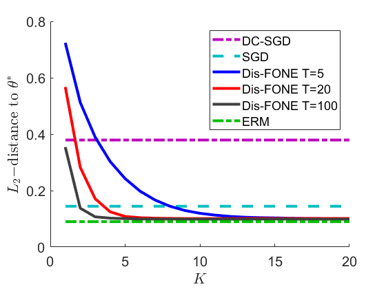
Moreover, by Condition (A1), we set the mini-batch size in DC-SGD (or the size of BtB_{t} in Dis-FONE, see Algorithm 3) as m=⌊p​log⁡n⌋m=\lfloor p\log n\rfloor, where ⌊x⌋\lfloor x\rfloor denotes the largest integer less than or equal to xx. For Dis-FONE, we first set the number of the iterations TT in each round as T=20T=20 and the number of rounds K=20K=20 for logistic regression and K=80K=80 for quantile regression. Note that due to the non-smoothness in the loss function of quantile regression, it requires more rounds of iterations KK to ensure the convergence. In practice, we could also adopt a simple data-driven approach to determine the number of rounds KK. In particular, we could stop the algorithm when the change (norm of the difference) between the estimators for two consecutive rounds is negligible. We carefully evaluate the effect of TT and KK (by considering different values of TT and KK) in Section 5.1.3. We also compare the methods with 𝜽^FONE\widehat{\bm{\theta}}_{\mathrm{FONE}} (Algorithm 2), which corresponds to the Dis-FONE 𝜽^dis,K\widehat{\bm{\theta}}_{\mathrm{dis},K} with only K=1K=1 round. All results reported below are based on the average of 100100 independent runs of simulations.

Table 1: Logistic regression: comparisons of L2L_{2}-errors when varying the total sample size NN and dimension pp changes. Here the number of machines L=20L=20. Denote by 𝜽^DC\widehat{\bm{\theta}}_{\mathrm{DC}} the DC-SGD estimator, 𝜽^SGD\widehat{\bm{\theta}}_{\mathrm{SGD}} the SGD estimator on the entire dataset in a non-distributed setting, 𝜽^FONE\widehat{\bm{\theta}}_{\mathrm{FONE}} the single-round FONE of Algorithm 2, and 𝜽^dis,K\widehat{\bm{\theta}}_{\mathrm{dis},K} the Dis-FONE with K=20K=20.
pp L2L_{2}-distance to the truth 𝜽∗\bm{\theta}^{*} L2L_{2}-distance to ERM 𝜽^\widehat{\bm{\theta}}
𝜽^0\widehat{\bm{\theta}}_{0} 𝜽^DC\widehat{\bm{\theta}}_{\mathrm{DC}} 𝜽^SGD\widehat{\bm{\theta}}_{\mathrm{SGD}} 𝜽^FONE\widehat{\bm{\theta}}_{\mathrm{FONE}} 𝜽^dis,K\widehat{\bm{\theta}}_{\mathrm{dis},K} 𝜽^\widehat{\bm{\theta}} 𝜽^DC\widehat{\bm{\theta}}_{\mathrm{DC}} 𝜽^SGD\widehat{\bm{\theta}}_{\mathrm{SGD}} 𝜽^dis,K\widehat{\bm{\theta}}_{\mathrm{dis},K}
N=105N=10^{5}
100 1.251 0.447 0.148 0.724 0.103 0.093 0.445 0.116 0.038
200 1.899 1.096 0.523 1.046 0.168 0.153 1.091 0.494 0.049
500 4.509 3.853 3.111 2.154 0.338 0.301 3.748 3.021 0.085
N=2×10⁵N=2\times 10^{5}
100 1.303 0.390 0.100 0.594 0.072 0.067 0.386 0.074 0.025
200 2.094 1.248 0.315 0.821 0.115 0.109 1.235 0.286 0.034
500 4.717 3.920 2.189 1.725 0.222 0.211 3.891 2.133 0.045
N=5×10⁵N=5\times 10^{5}
100 1.342 0.313 0.081 0.347 0.046 0.042 0.304 0.069 0.018
200 1.833 0.874 0.169 0.749 0.073 0.068 0.868 0.152 0.023
500 4.835 3.885 1.006 1.413 0.141 0.130 3.859 0.989 0.036
Table 2: Quantile regression: comparisons of L2L_{2}-errors when varying the total sample size NN and dimension pp. Here the number of machines L=20L=20. Denote by 𝜽^DC\widehat{\bm{\theta}}_{\mathrm{DC}} the DC-SGD estimator, 𝜽^SGD\widehat{\bm{\theta}}_{\mathrm{SGD}} the SGD estimator on the entire dataset in a non-distributed setting, 𝜽^FONE\widehat{\bm{\theta}}_{\mathrm{FONE}} the single-round FONE of Algorithm 2

, and 𝜽^dis,K\widehat{\bm{\theta}}_{\mathrm{dis},K} the Dis-FONE with K=80K=80.

pp L2L_{2}-distance to the truth 𝜽∗\bm{\theta}^{*} L2L_{2}-distance to ERM 𝜽^\widehat{\bm{\theta}}
𝜽^0\widehat{\bm{\theta}}_{0} 𝜽^DC\widehat{\bm{\theta}}_{\mathrm{DC}} 𝜽^SGD\widehat{\bm{\theta}}_{\mathrm{SGD}} 𝜽^FONE\widehat{\bm{\theta}}_{\mathrm{FONE}} 𝜽^dis,K\widehat{\bm{\theta}}_{\mathrm{dis},K} 𝜽^\widehat{\bm{\theta}} 𝜽^DC\widehat{\bm{\theta}}_{\mathrm{DC}} 𝜽^SGD\widehat{\bm{\theta}}_{\mathrm{SGD}} 𝜽^dis,K\widehat{\bm{\theta}}_{\mathrm{dis},K}
N=105N=10^{5}
100 0.450 0.079 0.063 0.191 0.047 0.043 0.073 0.050 0.020
200 0.715 0.114 0.109 0.342 0.082 0.071 0.106 0.097 0.035
500 1.278 0.198 0.176 0.554 0.144 0.126 0.176 0.142 0.062
N=2×10⁵N=2\times 10^{5}
100 0.450 0.070 0.037 0.130 0.035 0.030 0.067 0.021 0.015
200 0.726 0.101 0.067 0.246 0.059 0.054 0.098 0.037 0.027
500 1.287 0.176 0.118 0.379 0.098 0.076 0.157 0.065 0.046
N=5×10⁵N=5\times 10^{5}
100 0.451 0.043 0.030 0.114 0.029 0.025 0.037 0.017 0.014
200 0.719 0.067 0.047 0.157 0.041 0.037 0.064 0.026 0.020
500 1.294 0.105 0.076 0.264 0.074 0.057 0.091 0.041 0.035
Refer to caption
(a) Logistic regression: L2L_{2}-distance to 𝜽∗\bm{\theta}^{*}
Refer to caption
(b) Logistic regression: L2L_{2}-distance to 𝜽^\widehat{\bm{\theta}}
Refer to caption
(c) Quantile regression: L2L_{2}-distance to 𝜽∗\bm{\theta}^{*}
Refer to caption
(d) Quantile regression: L2L_{2}-distance to 𝜽^\widehat{\bm{\theta}}
Figure 1: Comparison of L2L_{2}-errors when NN increases. The left column reports the L2L_{2}-errors with respect to the truth 𝜽∗\bm{\theta}^{*} and the right column reports the L2L_{2}-errors with respect to the ERM 𝜽^\widehat{\bm{\theta}}. Here the dimension p=100p=100 and the number of machines L=20L=20. In Dis-FONE, we set K=20K=20 in the logistic regression case and K=80K=80 in the quantile regression case.

5.1.1 Effect of NN and pp

In Tables 1–2, we fix the number of machines L=20L=20 and vary the total sample size NN from {105,2×105,5×105}\{10^{5},2\times 10^{5},5\times 10^{5}\} and dimension p∈{100,200,500}p\in\{100,200,500\}. Results for logistic regression are reported in Table 1 and results for quantile regression are in Table 2. In both tables, the left columns provide the L2L_{2} estimation errors (with respect to the truth 𝜽∗\bm{\theta}^{*}) of the DC-SGD estimator 𝜽^DC\widehat{\bm{\theta}}_{\mathrm{DC}}, the SGD estimator 𝜽^SGD\widehat{\bm{\theta}}_{\mathrm{SGD}}, Dis-FONE 𝜽^dis,K\widehat{\bm{\theta}}_{\mathrm{dis},K}, and the ERM 𝜽^\widehat{\bm{\theta}}. We note that both SGD and ERM are non-distributed algorithms for pooled data. We will show that in many cases our distributed Dis-FONE estimator even outperforms the non-distributed SGD. For reference, we also report L2L_{2}-errors of the initial estimator 𝜽^0\widehat{\bm{\theta}}_{0}. The right columns report the L2L_{2}-distances to the ERM 𝜽^\widehat{\bm{\theta}}.

From Tables 1–2, we can see that the proposed Dis-FONE 𝜽^dis,K\widehat{\bm{\theta}}_{\mathrm{dis},K} achieves similar errors as the ERM 𝜽^\widehat{\bm{\theta}} in all cases, and outperforms DC-SGD and SGD especially when pp is large. We also provide Figure 1 that captures the performance of the estimators in terms of their L2L_{2}-errors when the total sample size NN increases. From Figure 1, we can see that the estimation error for each method decreases as NN increases. Moreover, the L2L_{2}-error of Dis-FONE is very close to the ERM as NN increases, while there is a significant gap between DC-SGD and the ERM.
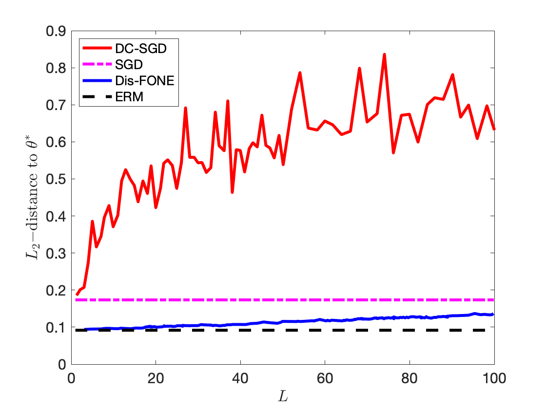
Refer to caption
(a) Logistic regression: L2L_{2}-distance to 𝜽∗\bm{\theta}^{*}
Refer to caption
(b) Logistic regression: L2L_{2}-distance to 𝜽^\widehat{\bm{\theta}}
Refer to caption
(c) Quantile regression: L2L_{2}-distance to 𝜽∗\bm{\theta}^{*}
Refer to caption
(d) Quantile regression: L2L_{2}-distance to 𝜽^\widehat{\bm{\theta}}
Figure 2: Comparison of L2L_{2}-errors when the number of machines LL increases. Here the total sample size N=105N=10^{5} and the dimension p=100p=100. Denote by 𝜽^dis,K\widehat{\bm{\theta}}_{\mathrm{dis},K} the Dis-FONE with K=20K=20 in the logistic regression case and K=80K=80 in the quantile regression case.

5.1.2 Effect on the number of machines LL

For the effect on the number of machines LL, we fix the total sample size N=105N=10^{5} and the dimension p=100p=100 and vary the number of machines LL from 11 to 200200, and plot the L2L_{2}-errors in Figure 2. From Figure 2, the L2L_{2}-error of DC-SGD increases as LL increases (i.e., each machine has fewer samples). In contrast, the L2L_{2}-error of Dis-FONE versus LL is almost flat, and is quite close to ERM even when LL is large. This is consistent with our theoretical result that DC-SGD will fail when LL is large. The SGD estimator, which is the L=1L=1 case of DC-SGD (and thus its error is irrelevant of LL and is presented by a horizontal line), provides moderate accuracy. Further increasing LL would lead to an excessively small local sample size (e.g., when N=105N=10^{5} and L>200L>200, we will have the local sample size n<500n<500, and thus is unrealistic in practice, considering that the dimensionality p=100p=100.

Refer to caption
(a) Logistic regression: L2L_{2}-distance to 𝜽∗\bm{\theta}^{*}
Refer to caption
(b) Logistic regression: L2L_{2}-distance to 𝜽^\widehat{\bm{\theta}}
Refer to caption
(c) Quantile regression: L2L_{2}-distance to 𝜽∗\bm{\theta}^{*}
Refer to caption
(d) Quantile regression: L2L_{2}-distance to 𝜽^\widehat{\bm{\theta}}
Figure 3: Comparison of L2L_{2}-errors when the number of rounds KK in Dis-FONE increases. The xx-axis is the number of rounds KK in Dis-FONE. Here the total sample size N=105N=10^{5}, the dimension p=100p=100, and the number of machines L=20L=20. The errors of DC-SGD, SGD, and ERM are presented by the horizontal lines since their performance is irrelevant of KK.

5.1.3 Effect of KK and TT in Dis-FONE

For Dis-FONE, we provide the comparison of the estimator errors with different numbers of rounds KK and numbers of inner iterations TT. In Figure 3, we fix the total sample size N=105N=10^{5}, the dimension p=100p=100, the number of machines L=20L=20 and vary TT from {5,20,100}\{5,20,100\}. The xx-axis in Figure 3 is the number of rounds KK. For all three cases of TT, the performance of Dis-FONE is quite desirable and reaches the accuracy of the ERM when KK becomes larger. When TT is smaller, it requires a larger KK for Dis-FONE to converge. In other words, we need to perform more rounds of Dis-FONE to achieve the same accuracy.

Refer to caption
(a) Logistic regression: L2L_{2}-distance to 𝜽∗\bm{\theta}^{*}
Refer to caption
(b) Logistic regression: L2L_{2}-distance to 𝜽^\widehat{\bm{\theta}}
Refer to caption
(c) Quantile regression: L2L_{2}-distance to 𝜽∗\bm{\theta}^{*}
Refer to caption
(d) Quantile regression: L2L_{2}-distance to 𝜽^\widehat{\bm{\theta}}
Figure 4: Comparison of L2L_{2}-errors when the sub-sample size of the first machine n1n_{1} in Dis-FONE increases. The xx-axis is the ratio of n1n_{1} to the total sample size NN. Here the total sample size N=105N=10^{5}, the dimension p=100p=100, and the number of machines L=20L=20.

5.1.4 Effect on the unbalanced data partition

In previous simulation studies, the entire dataset is evenly separated on different machines. As one can see from Algorithm 3 and Theorem 3.5, the sub-sample size on the first machine n1n_{1} plays a different role in Dis-FONE than those on the other machines n2,n3,…,nLn_{2},n_{3},\dots,n_{L}. In Figure 4, we investigate the effect of n1n_{1} by varying n1n_{1} from N/LN/L (the case of evenly distributed) to 10×N/L10\times N/L. Let the remaining data points be evenly distributed on the other machines, i.e., n2=n3=⋯=nL=(N−n1)/(L−1)n_{2}=n_{3}=\dots=n_{L}=(N-n_{1})/(L-1). We set N=105N=10^{5} and L=20L=20. From Figure 4, the L2L_{2}-error of Dis-FONE gets much closer to ERM 𝜽^\widehat{\bm{\theta}} in (2) when the largest sub-sample size n1n_{1} increases, which is consistent with our theoretical results.

In Appendix G, we further investigate the cases of correlated design, the effect of the quality of the initial estimator, and different choices of the stepsizes (see Section G for more details). We also conduct simulations to compare our proposed methods (DC-SGD and Dis-FONE) to the existing methods in Section G.4 in terms of statistical accuracy and computation time. For logistic regression, we compare our algorithm with CSL (Jordan et al. 2019) for logistic regression. Both Dis-FONE and CSL methods achieve nearly optimal performance as compared to the ERM, while Dis-FONE accelerates CSL. For quantile regression, we compare our methods with DC-QR (Volgushev et al. 2019). Dis-FONE outperforms DC-QR in terms of both computation time and statistical accuracy since DC-QR suffers from the restriction on the sub-sample size analogous to the case of DC-SGD.

5.1.5 Experiments on statistical inference

Table 3: Left columns: Coverage rates and average confidence interval length in the brackets; Right columns: Square roots of the ratios of the estimated variance to the true limiting variance of ERM 𝜽^\widehat{\bm{\theta}}. The sample size n∈{105,2×105,5×105}n\in\{10^{5},2\times 10^{5},5\times 10^{5}\} and dimension p∈{100,200,500}p\in\{100,200,500\}. The multiplier τn=((p​log⁡n)/n)1/2\tau_{n}=((p\log n)/n)^{1/2}, the step-size ηn=(p​log⁡n)/n\eta_{n}=(p\log n)/n for logistic regression, and τn=((p​log⁡n)/n)1/3\tau_{n}=((p\log n)/n)^{1/3}, ηn=((p​log⁡n)/n)2/3\eta_{n}=((p\log n)/n)^{2/3} for quantile regression, respectively.
Model     nn Coverage rates (Avg length) Square root ratio
p=100p=100 p=200p=200 p=500p=500 p=100p=100 p=200p=200 p=500p=500
Logistic
n=105n=10^{5} 94.37 (0.127) 93.76 (0.174) 91.67 (0.271) 1.043 1.033 1.027
n=2×10⁵n=2\times 10^{5} 94.49 (0.131) 94.10 (0.168) 92.14 (0.265) 1.041 1.027 1.019
n=5×10⁵n=5\times 10^{5} 94.71 (0.128) 94.23 (0.167) 92.31 (0.254) 1.017 1.017 1.014
Quantile
n=105n=10^{5} 94.57 (0.160) 94.11 (0.221) 92.96 (0.358) 1.042 1.023 1.027
n=2×10⁵n=2\times 10^{5} 94.64 (0.159) 94.24 (0.204) 93.04 (0.349) 1.007 1.004 1.004
n=5×10⁵n=5\times 10^{5} 94.67 (0.154) 94.59 (0.191) 93.47 (0.344) 1.005 1.002 1.003

In this section, we provide simulation studies for estimating 𝚺−1​𝒘\bm{\Sigma}^{-1}\bm{w}, where 𝚺\bm{\Sigma} is the population Hessian matrix of the underlying regression model and ‖𝒘‖2=1\|\bm{w}\|_{2}=1. As we illustrate in Section 4, this estimator plays an important role in estimating the limiting variance of the ERM.

In this experiment, we specify 𝒘=𝟏p/p\bm{w}=\bm{1}_{p}/\sqrt{p}, the sample size n∈{105,2×105,5×105}n\in\{10^{5},2\times 10^{5},5\times 10^{5}\}, the dimension p∈{100,200,500}p\in\{100,200,500\}. According to Theorems 4.1 and 4.2, we set the multiplier τn=((p​log⁡n)/n)1/2\tau_{n}=((p\log n)/n)^{1/2}, the step-size ηn=(p​log⁡n)/n\eta_{n}=(p\log n)/n for logistic regression, and τn=((p​log⁡n)/n)1/3\tau_{n}=((p\log n)/n)^{1/3}, ηn=((p​log⁡n)/n)2/3\eta_{n}=((p\log n)/n)^{2/3} for quantile regression, respectively.

Given 𝚺−1​𝒘^\widehat{\bm{\Sigma}^{-1}\bm{w}}, we are able to compute the estimator of limiting variance 𝒘′​𝚺−1​𝑨​𝚺−1​𝒘\bm{w}^{\prime}\bm{\Sigma}^{-1}\bm{A}\bm{\Sigma}^{-1}\bm{w} using (25). Based on that and (3), we construct the 95% confidence interval for 𝒘′​𝜽∗\bm{w}^{\prime}\bm{\theta}^{*} as follows,

𝒘′​𝜽^±Φ−1​(0.975)​𝒘′​𝚺−1​𝑨​𝚺−1​𝒘/n,\bm{w}^{\prime}\widehat{\bm{\theta}}\pm\Phi^{-1}(0.975)\sqrt{\bm{w}^{\prime}\bm{\Sigma}^{-1}\bm{A}\bm{\Sigma}^{-1}\bm{w}/n}, (28)

where Φ⁡(⋅)\Phi(\cdot) is the CDF of the standard normal random variable.

The left columns in Table 3 present the average coverage rates of the confidence intervals of 𝒘′​𝜽∗\bm{w}^{\prime}\bm{\theta}^{*} constructed by (28) and their average interval lengths. In the right columns of Table 3, we report the square root of the ratio between the estimated variance and the true limiting variance, i.e.,

(𝚺−1​𝒘^)′​𝑨^​(𝚺−1​𝒘^)/𝒘′​𝚺−1​𝑨​𝚺−1​𝒘.\sqrt{(\widehat{\bm{\Sigma}^{-1}\bm{w}})^{\prime}\widehat{\bm{A}}(\widehat{\bm{\Sigma}^{-1}\bm{w}})\Big/\bm{w}^{\prime}\bm{\Sigma}^{-1}\bm{A}\bm{\Sigma}^{-1}\bm{w}}.

From Table 3, our estimator achieves good performance for both logistic and quantile regression models. As the sample size nn increases, the coverage rates become closer to the nominal level and the ratios get closer to 11.

Refer to caption
(a) τ=0.25\tau=0.25: L2L_{2}-distance to 𝜽^\widehat{\bm{\theta}}
Refer to caption
(b) τ=0.5\tau=0.5: L2L_{2}-distance to 𝜽^\widehat{\bm{\theta}}
Figure 5: Real data analysis: comparison of L2L_{2}-errors when the sample size NN increases.

5.2 Real Data Analysis - Census 2000 Data

In this section, we provide real data analysis of our proposed methods. We consider the sampled U.S. 2000 Census dataset33 3 U.S. Census, http://www.census.gov/census2000/PUMS5.html, consisting of annual salary and related features on employed full-time wage and salary workers who reported that they worked 40 weeks or more and worked 35 hours or more per week. The U.S. 2000 Census dataset is a widely used dataset in quantile regression literature, see, e.g., Angrist et al. 2006; Yang et al. 2013. The entire sample size is 5×1065\times 10^{6} and the dimension p=11p=11. We perform a quantile regression on the dataset, which treats the annual salary as the response variable, with two different quantile levels τ=0.25\tau=0.25 and τ=0.5\tau=0.5 (i.e., the least absolute deviations regression). We use L=100L=100 machines/nodes and vary the total sample size NN from 5×1055\times 10^{5} to 5×1065\times 10^{6} to compare our Dis-FONE with DC-SGD in a distributed environment. In DC-SGD, we set α=1\alpha=1 in the step-size ri=c0/max⁡(iα,p)r_{i}=c_{0}/\max(i^{\alpha},p). In Dis-FONE, we set T=100T=100, K=20K=20, and step-size ηn=c0′​m/n\eta_{n}=c_{0}^{\prime}m/n. The constants c0c_{0} and c0′c_{0}^{\prime} is chosen in the say way as in the simulation study. More particularly, we choose the best c0c_{0} and c0′c_{0}^{\prime} that achieves the smallest objective function in (2) with 𝜽=𝜽^SGD(1)\bm{\theta}=\widehat{\bm{\theta}}_{\mathrm{SGD}}^{(1)} and 𝜽=𝜽^dis,1\bm{\theta}=\widehat{\bm{\theta}}_{\mathrm{dis},1} using data points from the first machine. The ERM estimator is computed by solving the quantile regression using the interior-point method with pooled data on a single powerful machine.

From Figure 5, our proposed Dis-FONE 𝜽^dis,K\widehat{\bm{\theta}}_{\mathrm{dis},K} is very close to the ERM estimator and outperforms both DC-SGD and SGD estimators. As NN increases, both DC-SGD and SGD estimators are closer to the ERM estimator. In addition to estimation accuracy, we further investigate the performance on the testing set. For a given NN, we split the data into the training set (with 0.8​N0.8N samples) and testing set (with 0.2​N0.2N). We estimate 𝜽^method\widehat{\bm{\theta}}_{\text{method}} using an estimation method, such as, DC-SGD, SGD, Dis-FONE, on the training set and evaluate the quantile objective value on the testing data. Denote the obtained quantile objective value on the testing set using a given method and the ERM by f^method\widehat{f}_{\text{method}} and f^ERM\widehat{f}_{\text{ERM}}, respectively. We report the relative errors of objective values |f^method−f^ERM|/|f^ERM||\widehat{f}_{\text{method}}-\widehat{f}_{\text{ERM}}|/|\widehat{f}_{\text{ERM}}| and from Figure 6, the relative errors of Dis-FONE are very close to zero.

Refer to caption
(a) τ=0.25\tau=0.25: relative errors of objective values
Refer to caption
(b) τ=0.5\tau=0.5: relative errors of objective values
Figure 6: Real data analysis: comparison of the relative errors of objective values |f^method−f^ERM|/|f^ERM||\widehat{f}_{\text{method}}-\widehat{f}_{\text{ERM}}|/|\widehat{f}_{\text{ERM}}| on the testing data when the sample size NN increases.

6 Conclusions

This paper studies general distributed estimation and inference problems based on stochastic subgradient descent. We propose an efficient First-Order Newton-type Estimator (FONE) for estimating 𝚺−1​𝒘\bm{\Sigma}^{-1}\bm{w} and its distributed version. The key idea behind our method is to use stochastic gradient information to approximate the Newton step. We further characterize the theoretical properties when using FONE for distributed estimation and inference with both smooth and non-smooth loss functions. We also conduct numerical studies to demonstrate the performance of the proposed distributed FONE. The proposed FONE of 𝚺−1​𝒘\bm{\Sigma}^{-1}\bm{w} is a general estimator, which could find applications to other statistical estimation problems. While this paper focuses on convex loss functions, the proposed methods can be directly applied to non-convex objectives. It would be an interesting future direction to derive the convergence rates for non-convex settings.

Acknowledgement

The authors are very grateful to anonymous referees and the associate editor for their detailed and constructive comments that considerably improved the quality of this paper. Xi Chen would like to thank the support from NSF via IIS-1845444. Weidong Liu is supported by National Program on Key Basic Research Project (973 Program, 2018AAA0100704), NSFC Grant No. 11825104 and 11690013, Youth Talent Support Program, and a grant from Australian Research Council.

Appendix A General Conditions and Their Verification

In this section, we first provide general versions of (A2-Log) and (A2-QR) beyond regression settings. In particular, the assumption (A2-Log) for logistic regression is generalized to conditions (C2) and (C3); and the assumption (A2-QR) for quantile regression is generalized to conditions (C2) and (C3∗).

Condition (C2) is on the continuity of subgradient g⁡(𝜽,𝝃)g(\bm{\theta},\bm{\xi}) and its expectation G⁡(𝜽):=𝔼​g​(𝜽,𝝃)G(\bm{\theta}):=\mathbb{E}g(\bm{\theta},\bm{\xi}). (C2). Suppose that G⁡(𝜽)G(\bm{\theta}) is differentiable on 𝜽\bm{\theta} and denote by 𝚺⁡(𝜽):=∇𝜽G​(𝜽)\bm{\Sigma}(\bm{\theta}):=\nabla_{\bm{\theta}}G(\bm{\theta}). For some constant C1>0C_{1}>0, we have

‖𝚺⁡(𝜽1)−𝚺⁡(𝜽2)‖≤C1​‖𝜽1−𝜽2‖2for any 𝜽1,𝜽2∈ℝp.\displaystyle\big\|\bm{\Sigma}(\bm{\theta}_{1})-\bm{\Sigma}(\bm{\theta}_{2})\big\|\leq C_{1}\|\bm{\theta}_{1}-\bm{\theta}_{2}\|_{2}\quad\mbox{for any $\bm{\theta}_{1},\bm{\theta}_{2}\in\mathbb{R}^{p}$.} (29)

Furthermore, let λmin​(𝚺​(𝜽))\lambda_{\min}(\bm{\Sigma}(\bm{\theta})) and λmax​(𝚺​(𝜽))\lambda_{\max}(\bm{\Sigma}(\bm{\theta})) be the minimum and maximum eigenvalue of 𝚺⁡(𝜽)\bm{\Sigma}(\bm{\theta}), respectively. We assume that c1≤λmin​(𝚺⁡(𝜽∗))≤λmax​(𝚺⁡(𝜽∗))≤c1−1c_{1}\leq\lambda_{\min}(\bm{\Sigma}(\bm{\theta}^{*}))\leq\lambda_{\max}(\bm{\Sigma}(\bm{\theta}^{*}))\leq c^{-1}_{1} for some constant c1>0c_{1}>0.

Condition (C2) can be easily verified in our two motivating examples of logistic regression and quantile regression (see Section A.1 below). It is worthwhile to note that 𝚺\bm{\Sigma} defined in (4) is a brief notation for 𝚺⁡(𝜽∗)\bm{\Sigma}(\bm{\theta}^{*}). The minimum eigenvalue condition on 𝚺⁡(𝜽∗)\bm{\Sigma}(\bm{\theta}^{*}) (i.e., λmin​(𝚺⁡(𝜽∗))≥c1\lambda_{\min}(\bm{\Sigma}(\bm{\theta}^{*}))\geq c_{1}) ensures that the population risk F⁡(𝜽)F(\bm{\theta}) is locally strongly convex at 𝜽=𝜽∗\bm{\theta}=\bm{\theta}^{*}.

(C3). (For smooth loss function ff) For 𝒗∈ℝp\bm{v}\in\mathbb{R}^{p}, assume that

|𝒗[g(𝜽1,𝝃)−g(𝜽2,𝝃)]′|≤U(𝒗,𝜽1,𝜽2)∥𝜽1−𝜽2∥2,\big|\bm{v}{{}^{\prime}}[g(\bm{\theta}_{1},\bm{\xi})-g(\bm{\theta}_{2},\bm{\xi})]\big|\leq U(\bm{v},\bm{\theta}_{1},\bm{\theta}_{2})\|\bm{\theta}_{1}-\bm{\theta}_{2}\|_{2},

where U⁡(𝒗,𝜽1,𝜽2)U(\bm{v},\bm{\theta}_{1},\bm{\theta}_{2}) satisfies that

sup‖𝒗‖2=1sup𝜽1,𝜽2𝔼​exp⁡(t0​U​(𝒗,𝜽1,𝜽2))≤C,sup‖𝒗‖2=1𝔼​sup𝜽1,𝜽2U⁡(𝒗,𝜽1,𝜽2)≤pc2,\sup_{\|\bm{v}\|_{2}=1}\sup_{\bm{\theta}_{1},\bm{\theta}_{2}}\mathbb{E}\exp\big(t_{0}U(\bm{v},\bm{\theta}_{1},\bm{\theta}_{2})\big)\leq C,\qquad\sup_{\|\bm{v}\|_{2}=1}\mathbb{E}\sup_{\bm{\theta}_{1},\bm{\theta}_{2}}U(\bm{v},\bm{\theta}_{1},\bm{\theta}_{2})\leq p^{c_{2}},

for some c2,t0,C>0c_{2},t_{0},C>0. Moreover, one of the following two conditions on g⁡(𝜽,𝝃)g(\bm{\theta},\bm{\xi}) holds,

  1. 1.

    sup‖𝒗‖2=1𝔼​sup𝜽exp⁡(t0​|𝒗′​g​(𝜽,𝝃)|)≤C\sup_{\|\bm{v}\|_{2}=1}\mathbb{E}\sup_{\bm{\theta}}\exp(t_{0}|\bm{v}^{\prime}g(\bm{\theta},\bm{\xi})|)\leq C for some t0,C>0t_{0},C>0;

  2. 2.

    sup‖𝒗‖2=1𝔼​exp⁡(t0​|𝒗′​g​(𝜽∗,𝝃)|)≤C\sup_{\|\bm{v}\|_{2}=1}\mathbb{E}\exp(t_{0}|\bm{v}^{\prime}g(\bm{\theta}^{*},\bm{\xi})|)\leq C and c1≤λmin​(𝚺⁡(𝜽))≤λmax​(𝚺⁡(𝜽))≤c1−1c_{1}\leq\lambda_{\min}(\bm{\Sigma}(\bm{\theta}))\leq\lambda_{\max}(\bm{\Sigma}(\bm{\theta}))\leq c_{1}^{-1} uniformly in 𝜽\bm{\theta} for some t0,c1,C>0t_{0},c_{1},C>0.

(C3∗). (For non-smooth loss function ff) Suppose that for some constant c2,c3,c4>0c_{2},c_{3},c_{4}>0,

sup𝜽1:‖𝜽1−𝜽∗‖2≤c4𝔼{sup𝜽2:‖𝜽1−𝜽2‖2≤n−M,‖𝜽2−𝜽∗‖2≤c4∥g(𝜽1,𝝃)−g(𝜽2,𝝃)∥24}≤pc2n−c3​M\sup_{\bm{\theta}_{1}:\|\bm{\theta}_{1}-\bm{\theta}^{*}\|_{2}\leq c_{4}}\mathbb{E}\big\{\sup_{\bm{\theta}_{2}:\|\bm{\theta}_{1}-\bm{\theta}_{2}\|_{2}\leq n^{-M},\;\|\bm{\theta}_{2}-\bm{\theta}^{*}\|_{2}\leq c_{4}}\|g(\bm{\theta}_{1},\bm{\xi})-g(\bm{\theta}_{2},\bm{\xi})\|_{2}^{4}\Big\}\leq p^{c_{2}}n^{-c_{3}M}

for any large M>0M>0. Also

sup‖𝒗‖2=1𝔼⁡(𝒗′​(g⁡(𝜽1,𝝃)−g⁡(𝜽2,𝝃))2​exp​{t0​|𝒗′​(g⁡(𝜽1,𝝃)−g⁡(𝜽2,𝝃))|}≤C​‖𝜽1−𝜽2‖2CLOSE\displaystyle\sup_{\|\bm{v}\|_{2}=1}\mathbb{E}(\bm{v}^{\prime}(g(\bm{\theta}_{1},\bm{\xi})-g(\bm{\theta}_{2},\bm{\xi}))^{2}\exp\{t_{0}|\bm{v}^{\prime}(g(\bm{\theta}_{1},\bm{\xi})-g(\bm{\theta}_{2},\bm{\xi}))|\}\leq C\|\bm{\theta}_{1}-\bm{\theta}_{2}\|_{2}

and sup‖𝒗‖2=1𝔼​sup𝜽exp⁡(t0​|𝒗′​g​(𝜽,𝝃)|)≤C\sup_{\|\bm{v}\|_{2}=1}\mathbb{E}\sup_{\bm{\theta}}\exp(t_{0}|\bm{v}^{\prime}g(\bm{\theta},\bm{\xi})|)\leq C for some t0t_{0}, C>0C>0.

In Condition (C3), we only require either one of the two bullets of the conditions on g⁡(𝜽,𝝃)g(\bm{\theta},\bm{\xi}) to hold. The second bullet in Condition (C3) requires the moment condition on the subgradient g⁡(𝜽∗,𝝃)g(\bm{\theta}^{*},\bm{\xi}) holds at the true parameter 𝜽∗\bm{\theta}^{*}, and weakens the uniform moment condition in the first bullet. On the other hand, it imposes an extra condition on the uniform eigenvalue bound of the matrix 𝚺⁡(𝜽)\bm{\Sigma}(\bm{\theta}), which is equivalent to assuming that the loss function ff is strongly convex on its entire domain. It is also worthwhile noting that the second bullet covers the case of linear regression where 𝚺⁡(𝜽)=𝑿​𝑿′/n\bm{\Sigma}(\bm{\theta})=\bm{X}\bm{X}^{\prime}/n for all 𝜽\bm{\theta}.

A.1 Verification of Conditions on Motivating Examples

In this section, we provide verification of the conditions (C2), (C3) and (C3∗) on Examples 2.1 and 2.2.

Example 2.1.

For a logistic regression model with 𝛏=(Y,𝐗)\bm{\xi}=(Y,\bm{X}),

ℙ⁡(Y=1|𝑿)=1−ℙ⁡(Y=−1|𝑿)=11+exp⁡(−𝑿′​𝜽∗).\displaystyle\mathbb{P}(Y=1|\bm{X})=1-\mathbb{P}(Y=-1|\bm{X})=\frac{1}{1+\mathrm{exp}(-\bm{X}^{\prime}\bm{\theta}^{*})}.

We have f⁡(𝛉,𝛏)=log⁡(1+exp⁡(−Y​𝐗′​𝛉))f(\bm{\theta},\bm{\xi})=\log(1+\exp(-Y\bm{X}^{\prime}\bm{\theta})), and g⁡(𝛉,𝛏)=−Y​𝐗1+exp⁡(Y​𝐗′​𝛉)g(\bm{\theta},\bm{\xi})=\frac{-Y\bm{X}}{1+\exp(Y\bm{X}^{\prime}\bm{\theta})}. Note that G⁡(𝛉)=𝔼⁡(𝐗1+e−𝐗′​𝛉∗−𝐗1+e−𝐗′​𝛉)G(\bm{\theta})=\mathbb{E}\left(\frac{\bm{X}}{1+e^{-\bm{X}^{\prime}\bm{\theta}^{*}}}-\frac{\bm{X}}{1+e^{-\bm{X}^{\prime}\bm{\theta}}}\right) is differentiable in 𝛉\bm{\theta}. Moreover, we have,

𝚺⁡(𝜽)=𝔼​𝑿​𝑿′[1+exp⁡(𝑿′​𝜽)]​[1+exp⁡(−𝑿′​𝜽)].\bm{\Sigma}(\bm{\theta})=\mathbb{E}\frac{\bm{X}\bm{X}^{\prime}}{[1+\exp({\bm{X}^{\prime}\bm{\theta}})][1+\exp(-{\bm{X}^{\prime}\bm{\theta}})]}.
Proposition A.1.

In Example 2.1, assume that c~1≤λmin(𝔼(𝐗𝐗′))≤λmax(𝔼(𝐗𝐗′))≤c~1−1\widetilde{c}_{1}\leq\lambda_{\min}(\mathbb{E}(\bm{X}\bm{X}^{{}^{\prime}}))\leq\lambda_{\max}(\mathbb{E}(\bm{X}\bm{X}^{{}^{\prime}}))\leq\widetilde{c}^{-1}_{1} for some c~1>0\widetilde{c}_{1}>0 and sup‖𝐯‖2=1𝔼|𝐯′𝐗|3≤C~1\sup_{\|\bm{v}\|_{2}=1}\mathbb{E}|\bm{v}^{{}^{\prime}}\bm{X}|^{3}\leq\widetilde{C}_{1} for some C~1>0\widetilde{C}_{1}>0.

  1. (1)

    We have λmax​(𝚺​(𝜽))\lambda_{\max}(\bm{\Sigma}(\bm{\theta})) is bounded uniformly in 𝜽\bm{\theta}. Furthermore, if ‖𝜽∗‖2≤C~2\|\bm{\theta}^{*}\|_{2}\leq\widetilde{C}_{2}, then λmin​(𝚺⁡(𝜽∗))≥c1\lambda_{\min}(\bm{\Sigma}(\bm{\theta}^{*}))\geq c_{1} for some c1>0c_{1}>0 and (C2) holds.

  2. (2)

    If the covariates 𝑿\bm{X} satisfy sup‖𝒗‖2=1𝔼exp(t0(𝒗′𝑿)2)≤C~2\sup_{\|\bm{v}\|_{2}=1}\mathbb{E}\exp(t_{0}(\bm{v}^{{}^{\prime}}\bm{X})^{2})\leq\widetilde{C}_{2} for some t0,C~2>0t_{0},\widetilde{C}_{2}>0, then (C3) holds.

Proof. Note that

∥𝚺(𝜽)∥22=sup‖𝒗‖2=1𝔼(𝒗′𝑿)2[1+exp⁡(𝑿′​𝜽)]​[1+exp⁡(−𝑿′​𝜽)]≤sup‖𝒗‖2=1𝔼(𝒗′𝑿)2≤c~1−1.\displaystyle\|\bm{\Sigma}(\bm{\theta})\|^{2}_{2}=\sup_{\|\bm{v}\|_{2}=1}\mathbb{E}\frac{(\bm{v}^{{}^{\prime}}\bm{X})^{2}}{[1+\exp({\bm{X}^{\prime}\bm{\theta}})][1+\exp(-{\bm{X}^{\prime}\bm{\theta}})]}\leq\sup_{\|\bm{v}\|_{2}=1}\mathbb{E}(\bm{v}^{{}^{\prime}}\bm{X})^{2}\leq\widetilde{c}^{-1}_{1}.

That is, λmax​(𝚺​(𝜽))\lambda_{\max}(\bm{\Sigma}(\bm{\theta})) is bounded uniformly in 𝜽\bm{\theta}. Also,

λmin​(𝚺⁡(𝜽∗))\displaystyle\lambda_{\min}(\bm{\Sigma}(\bm{\theta}^{*})) =\displaystyle= min‖𝒗‖2=1⁡𝔼​(𝒗′𝑿)2[1+exp⁡(𝑿′​𝜽∗)]​[1+exp⁡(−𝑿′​𝜽∗)]\displaystyle\min_{\|\bm{v}\|_{2}=1}\mathbb{E}\frac{(\bm{v}^{{}^{\prime}}\bm{X})^{2}}{[1+\exp({\bm{X}^{\prime}\bm{\theta}^{*}})][1+\exp(-{\bm{X}^{\prime}\bm{\theta}^{*}})]}
≥\displaystyle\geq min‖𝒗‖2=1𝔼(𝒗′𝑿)22​(1+eM)I{|𝑿′𝜽∗|≤M}\displaystyle\min_{\|\bm{v}\|_{2}=1}\mathbb{E}\frac{(\bm{v}^{{}^{\prime}}\bm{X})^{2}}{2(1+e^{M})}I\{|\bm{X}^{{}^{\prime}}\bm{\theta}^{*}|\leq M\}
=\displaystyle= 12​(1+eM)min‖𝒗‖2=1(𝔼(𝒗′𝑿)2−𝔼(𝒗′𝑿)2I{|𝑿′𝜽∗|>M})\displaystyle\frac{1}{2(1+e^{M})}\min_{\|\bm{v}\|_{2}=1}\Big(\mathbb{E}(\bm{v}^{{}^{\prime}}\bm{X})^{2}-\mathbb{E}(\bm{v}^{{}^{\prime}}\bm{X})^{2}I\{|\bm{X}^{{}^{\prime}}\bm{\theta}^{*}|>M\}\Big)
≥\displaystyle\geq 12​(1+eM)min‖𝒗‖2=1(𝔼(𝒗′𝑿)2−C~1​C~2M)\displaystyle\frac{1}{2(1+e^{M})}\min_{\|\bm{v}\|_{2}=1}\Big(\mathbb{E}(\bm{v}^{{}^{\prime}}\bm{X})^{2}-\frac{\widetilde{C}_{1}\widetilde{C}_{2}}{M}\Big)
=\displaystyle= 12​(1+eM)​(c~1−M−1​C~1​C~2).\displaystyle\frac{1}{2(1+e^{M})}\Big(\widetilde{c}_{1}-M^{-1}\widetilde{C}_{1}\widetilde{C}_{2}\Big).

Now let MM be a constant that satisfies M>C~1​C~2/c~1M>\widetilde{C}_{1}\widetilde{C}_{2}/\widetilde{c}_{1}. This yields that λmin​(𝚺⁡(𝜽∗))≥c1\lambda_{\min}(\bm{\Sigma}(\bm{\theta}^{*}))\geq c_{1} for some c1>0c_{1}>0. By noting that the derivative of (1+ex)−1​(1+e−x)−1(1+e^{x})^{-1}(1+e^{-x})^{-1} is bounded by 33, we have

∥𝚺(𝜽1)−𝚺(𝜽2)∥≤3sup‖𝒗‖2=1𝔼(𝒗′𝑿)2|𝑿′(𝜽1−𝜽2)|≤3C~1∥𝜽1−𝜽2∥2.\displaystyle\|\bm{\Sigma}(\bm{\theta}_{1})-\bm{\Sigma}(\bm{\theta}_{2})\|\leq 3\sup_{\|\bm{v}\|_{2}=1}\mathbb{E}(\bm{v}^{{}^{\prime}}\bm{X})^{2}|\bm{X}^{{}^{\prime}}(\bm{\theta}_{1}-\bm{\theta}_{2})|\leq 3\widetilde{C}_{1}\|\bm{\theta}_{1}-\bm{\theta}_{2}\|_{2}.

This proves (C2). Similarly, the derivative of (1+ex)−1(1+e^{x})^{-1} is bounded by 1, and hence for 𝜽1≠𝜽2\bm{\theta}_{1}\neq\bm{\theta}_{2},

|𝒗′g(𝜽1,𝝃)−𝒗′g(𝜽2,𝝃)|≤|𝒗′𝑿||𝑿′(𝜽1−𝜽2)|≤U(𝒗,𝜽1,𝜽2)∥𝜽1−𝜽2∥2,\displaystyle|\bm{v}^{{}^{\prime}}g(\bm{\theta}_{1},\bm{\xi})-\bm{v}^{{}^{\prime}}g(\bm{\theta}_{2},\bm{\xi})|\leq|\bm{v}^{{}^{\prime}}\bm{X}||\bm{X}^{{}^{\prime}}(\bm{\theta}_{1}-\bm{\theta}_{2})|\leq U(\bm{v},\bm{\theta}_{1},\bm{\theta}_{2})\|\bm{\theta}_{1}-\bm{\theta}_{2}\|_{2},

where U(𝒗,𝜽1,𝜽2)=|𝒗′𝑿||𝑿′(𝜽1−𝜽2)|/∥𝜽1−𝜽2∥2U(\bm{v},\bm{\theta}_{1},\bm{\theta}_{2})=|\bm{v}^{{}^{\prime}}\bm{X}||\bm{X}^{{}^{\prime}}(\bm{\theta}_{1}-\bm{\theta}_{2})|/\|\bm{\theta}_{1}-\bm{\theta}_{2}\|_{2}. It is easy to see that

sup‖𝒗‖2=1sup𝜽1,𝜽2𝔼​exp⁡(t0​U​(𝒗,𝜽1,𝜽2))≤sup‖𝒗‖2=1𝔼​exp⁡(t0​(𝒗′​𝑿)2)≤C~2,\sup_{\|\bm{v}\|_{2}=1}\sup_{\bm{\theta}_{1},\bm{\theta}_{2}}\mathbb{E}\exp(t_{0}U(\bm{v},\bm{\theta}_{1},\bm{\theta}_{2}))\leq\sup_{\|\bm{v}\|_{2}=1}\mathbb{E}\exp(t_{0}(\bm{v}^{\prime}\bm{X})^{2})\leq\widetilde{C}_{2},

and

sup‖𝒗‖2=1𝔼​sup𝜽1,𝜽2U⁡(𝒗,𝜽1,𝜽2)≤sup‖𝒗‖2=1𝔼​sup‖𝜽‖2=1|𝒗′​𝑿|​|𝜽′​𝑿|≤C​p.\sup_{\|\bm{v}\|_{2}=1}\mathbb{E}\sup_{\bm{\theta}_{1},\bm{\theta}_{2}}U(\bm{v},\bm{\theta}_{1},\bm{\theta}_{2})\leq\sup_{\|\bm{v}\|_{2}=1}\mathbb{E}\sup_{\|\bm{\theta}\|_{2}=1}|\bm{v}^{\prime}\bm{X}||\bm{\theta}^{\prime}\bm{X}|\leq Cp.

Therefore, U⁡(𝒗,𝜽1,𝜽2)U(\bm{v},\bm{\theta}_{1},\bm{\theta}_{2}) satisfies (C3). At the meantime, since |𝒗′​g​(𝜽,𝝃)|≤|𝒗′​𝑿||\bm{v}^{\prime}g(\bm{\theta},\bm{\xi})|\leq|\bm{v}^{\prime}\bm{X}| for any 𝜽\bm{\theta}, and sup‖𝒗‖2=1𝔼exp(t0(𝒗′𝑿)2)≤C~2\sup_{\|\bm{v}\|_{2}=1}\mathbb{E}\exp(t_{0}(\bm{v}^{{}^{\prime}}\bm{X})^{2})\leq\widetilde{C}_{2} for some t0,C~2>0t_{0},\widetilde{C}_{2}>0, bullet (1) of (C3) holds for g⁡(𝜽,𝝃)g(\bm{\theta},\bm{\xi}).∎

Example 2.2.

For a quantile regression model,

y=𝑿′​𝜽∗+ϵ,ℙ⁡(ϵ≤0|𝑿)=τ.\displaystyle y=\bm{X}^{\prime}\bm{\theta}^{*}+\epsilon,\qquad\mathbb{P}(\epsilon\leq 0|\bm{X})=\tau.

We have the non-smooth quantile loss f⁡(𝛉,𝛏)=ℓ⁡(y−𝐗′​𝛉)f(\bm{\theta},\bm{\xi})=\ell(y-\bm{X}^{\prime}\bm{\theta}) with ℓ(x)=x(τ−I{x≤0}))\ell(x)=x(\tau-I\{x\leq 0\})), and its subgradient g(𝛉,𝛏)=𝐗(I{y≤𝐗′𝛉}−τ)g(\bm{\theta},\bm{\xi})=\bm{X}(I\{y\leq\bm{X}^{\prime}\bm{\theta}\}-\tau). Then G⁡(𝛉)=𝔼⁡[𝐗⁡(ℙ⁡(ϵ≤𝐗′​(𝛉−𝛉∗)|𝐗)−τ)]G(\bm{\theta})=\mathbb{E}[\bm{X}(\mathbb{P}(\epsilon\leq\bm{X}^{\prime}(\bm{\theta}-\bm{\theta}^{*})|\bm{X})-\tau)]. Furthermore, we have 𝚺⁡(𝛉)=𝔼⁡[𝐗​𝐗′​ρ𝐗​(𝐗′​(𝛉−𝛉∗))]\bm{\Sigma}(\bm{\theta})=\mathbb{E}[\bm{X}\bm{X}^{\prime}\rho_{\bm{X}}(\bm{X}^{\prime}(\bm{\theta}-\bm{\theta}^{*}))], where ρ𝐗​(⋅)\rho_{\bm{X}}(\cdot) is the density function of ϵ\epsilon given 𝐗\bm{X}.

Proposition A.2.

Assume that

c1≤λmin​(𝔼⁡[𝑿​𝑿′​ρ𝑿​(0)])≤λmax​(𝔼⁡[𝑿​𝑿′​ρ𝑿​(0)])≤c1−1c_{1}\leq\lambda_{\min}(\mathbb{E}[\bm{X}\bm{X}^{\prime}\rho_{\bm{X}}(0)])\leq\lambda_{\max}(\mathbb{E}[\bm{X}\bm{X}^{\prime}\rho_{\bm{X}}(0)])\leq c^{-1}_{1}

for some c1>0c_{1}>0 and sup‖𝐯‖2=1𝔼|𝐯′𝐗|3≤C~1\sup_{\|\bm{v}\|_{2}=1}\mathbb{E}|\bm{v}^{{}^{\prime}}\bm{X}|^{3}\leq\widetilde{C}_{1} for some C~1>0\widetilde{C}_{1}>0. The density function ρ𝐗​(x)\rho_{\bm{X}}(x) is bounded and satisfies |ρ𝐗​(x1)−ρ𝐗​(x2)|≤C~​|x1−x2||\rho_{\bm{X}}(x_{1})-\rho_{\bm{X}}(x_{2})|\leq\widetilde{C}|x_{1}-x_{2}| for some C~>0\widetilde{C}>0. Then (C2) holds. Furthermore, if the covariates 𝐗\bm{X} satisfy sup‖𝐯‖2=1𝔼exp(t0|𝐯′𝐗|)≤C~2\sup_{\|\bm{v}\|_{2}=1}\mathbb{E}\exp(t_{0}|\bm{v}^{{}^{\prime}}\bm{X}|)\leq\widetilde{C}_{2}, then (C3∗) holds.

Proof. By the Lipschitz condition on ρ𝑿​(x)\rho_{\bm{X}}(x), we have

∥𝚺(𝜽1)−𝚺(𝜽2)∥2≤C~sup‖𝒗‖2=1𝔼(𝒗′𝑿)2|𝑿′(𝜽1−𝜽2)|≤C~1C~∥𝜽1−𝜽2∥2.\displaystyle\|\bm{\Sigma}(\bm{\theta}_{1})-\bm{\Sigma}(\bm{\theta}_{2})\|_{2}\leq\widetilde{C}\sup_{\|\bm{v}\|_{2}=1}\mathbb{E}(\bm{v}^{{}^{\prime}}\bm{X})^{2}|\bm{X}^{{}^{\prime}}(\bm{\theta}_{1}-\bm{\theta}_{2})|\leq\widetilde{C}_{1}\widetilde{C}\|\bm{\theta}_{1}-\bm{\theta}_{2}\|_{2}.

Hence (C2) holds. Now we prove (C3∗). Since ρ𝑿​(x)\rho_{\bm{X}}(x) is bounded, we have

𝔼[sup𝜽2:‖𝜽1−𝜽2‖2≤n−M,‖𝜽2−𝜽∗‖2≤c4∥g(𝜽1,𝝃)−g(𝜽2,𝝃)∥24]\displaystyle\mathbb{E}\big[\sup_{\bm{\theta}_{2}:\|\bm{\theta}_{1}-\bm{\theta}_{2}\|_{2}\leq n^{-M},\;\|\bm{\theta}_{2}-\bm{\theta}^{*}\|_{2}\leq c_{4}}\|g(\bm{\theta}_{1},\bm{\xi})-g(\bm{\theta}_{2},\bm{\xi})\|_{2}^{4}\big]
≤𝔼[∥𝑿∥24I{|𝑿′(𝜽1−𝜽∗)|−∥𝑿∥2n−M≤ϵ≤|𝑿′(𝜽1−𝜽∗)|+∥𝑿∥2n−M}]\displaystyle\leq\mathbb{E}\Big[\|\bm{X}\|_{2}^{4}I\big\{|\bm{X}^{\prime}(\bm{\theta}_{1}-\bm{\theta}^{*})|-\|\bm{X}\|_{2}n^{-M}\leq\epsilon\leq|\bm{X}^{\prime}(\bm{\theta}_{1}-\bm{\theta}^{*})|+\|\bm{X}\|_{2}n^{-M}\big\}\Big]
≤2​C~​𝔼​[‖𝑿‖25​n−M]\displaystyle\leq 2\widetilde{C}\mathbb{E}\big[\|\bm{X}\|_{2}^{5}n^{-M}\big]
≤2​C~​p5/2​n−M.\displaystyle\leq 2\widetilde{C}p^{5/2}n^{-M}.

Again,

𝔼⁡(𝒗′​(g⁡(𝜽1,𝝃)−g⁡(𝜽2,𝝃))2​exp​{t0​|𝒗′​(g⁡(𝜽1,𝝃)−g⁡(𝜽2,𝝃))|}CLOSE\displaystyle\mathbb{E}(\bm{v}^{\prime}(g(\bm{\theta}_{1},\bm{\xi})-g(\bm{\theta}_{2},\bm{\xi}))^{2}\exp\{t_{0}|\bm{v}^{\prime}(g(\bm{\theta}_{1},\bm{\xi})-g(\bm{\theta}_{2},\bm{\xi}))|\}
≤𝔼[(𝒗′𝑿)2(I{ϵ≤𝑿′(𝜽1−𝜽∗)}−I{ϵ≤𝑿′(𝜽2−𝜽∗)})2exp{t0|𝒗′𝑿|}]\displaystyle\quad\leq\mathbb{E}\Big[(\bm{v}^{\prime}\bm{X})^{2}(I\{\epsilon\leq\bm{X}^{{}^{\prime}}(\bm{\theta}_{1}-\bm{\theta}^{*})\}-I\{\epsilon\leq\bm{X}^{{}^{\prime}}(\bm{\theta}_{2}-\bm{\theta}^{*})\})^{2}\exp\{t_{0}|\bm{v}^{\prime}\bm{X}|\}\Big]
≤𝔼[(𝒗′𝑿)2I{𝑿′(𝜽1−𝜽∗)≤ϵ≤𝑿′(𝜽2−𝜽∗)}exp{t0|𝒗′𝑿|}]\displaystyle\quad\leq\mathbb{E}\Big[(\bm{v}^{\prime}\bm{X})^{2}I\big\{\bm{X}^{{}^{\prime}}(\bm{\theta}_{1}-\bm{\theta}^{*})\leq\epsilon\leq\bm{X}^{{}^{\prime}}(\bm{\theta}_{2}-\bm{\theta}^{*})\big\}\exp\{t_{0}|\bm{v}^{\prime}\bm{X}|\}\Big]
+𝔼[(𝒗′𝑿)2I{𝑿′(𝜽2−𝜽∗)≤ϵ≤𝑿′(𝜽1−𝜽∗)}exp{t0|𝒗′𝑿|}]\displaystyle\qquad+\mathbb{E}\Big[(\bm{v}^{\prime}\bm{X})^{2}I\big\{\bm{X}^{{}^{\prime}}(\bm{\theta}_{2}-\bm{\theta}^{*})\leq\epsilon\leq\bm{X}^{{}^{\prime}}(\bm{\theta}_{1}-\bm{\theta}^{*})\big\}\exp\{t_{0}|\bm{v}^{\prime}\bm{X}|\}\Big]
≤2C~𝔼[(𝒗′𝑿)2|𝑿′(𝜽1−𝜽2)|exp{t0|𝒗′𝑿|}]\displaystyle\quad\leq 2\widetilde{C}\mathbb{E}\Big[(\bm{v}^{\prime}\bm{X})^{2}|\bm{X}^{{}^{\prime}}(\bm{\theta}_{1}-\bm{\theta}_{2})|\exp\{t_{0}|\bm{v}^{\prime}\bm{X}|\}\Big]
≤C​‖𝜽1−𝜽2‖2,\displaystyle\quad\leq C\|\bm{\theta}_{1}-\bm{\theta}_{2}\|_{2},

for some C>0C>0. This ensures that (C3∗) holds.∎

Appendix B Theory of Mini-batch SGD

Before we prove the theory of DC-SGD, we first provide some theoretical results of the mini-batch SGD in the diverging pp case. In particular, let 𝔼0​(⋅)\mathbb{E}_{0}(\cdot) be the expectation to {𝝃i,1≤i≤n}\{\bm{\xi}_{i},1\leq i\leq n\} given the initial estimator 𝜽^0\widehat{\bm{\theta}}_{0}. Let us denote the solution of mini-batch SGD in (6) with s=n/ms=n/m iterations by 𝜽^SGD\widehat{\bm{\theta}}_{\mathrm{SGD}}. We obtain the consistency result of the mini-batch SGD in the diverging pp case. Recall that ri=c0/max⁡(iα,p)r_{i}=c_{0}/\max(i^{\alpha},p) for some 0<α≤10<\alpha\leq 1 and c0c_{0} is a sufficiently large constant.

Theorem B.1.

Assume (C1), (C2), (C3) or (C3∗) hold and the initial estimator 𝛉^0\widehat{\bm{\theta}}_{0} is independent to {𝛏i,i=1,2,…,n}\{\bm{\xi}_{i},i=1,2,\dots,n\}. On the event {∥𝛉^0−𝛉∗∥2≤dn}\{\|\widehat{\bm{\theta}}_{0}-\bm{\theta}^{*}\|_{2}\leq d_{n}\} with dn→0d_{n}\rightarrow 0, the mini-batch SGD estimator satisfies

𝔼0​‖𝜽^SGD−𝜽∗‖22=O⁡(pm1−α​nα)and‖𝔼0​(𝜽^SGD)−𝜽∗‖2=O⁡(pm1−α​nα).\mathbb{E}_{0}\|\widehat{\bm{\theta}}_{\mathrm{SGD}}-\bm{\theta}^{*}\|_{2}^{2}=O(\frac{p}{m^{1-\alpha}n^{\alpha}})\quad\text{and}\quad\|\mathbb{E}_{0}(\widehat{\bm{\theta}}_{\mathrm{SGD}})-\bm{\theta}^{*}\|_{2}=O(\frac{p}{m^{1-\alpha}n^{\alpha}}).

Furthermore, if ‖𝛉^0−𝛉∗‖2=oℙ​(1)\|\widehat{\bm{\theta}}_{0}-\bm{\theta}^{*}\|_{2}=o_{\mathbb{P}}(1), then ‖𝛉^SGD−𝛉∗‖22=Oℙ​(pm1−α​nα)\|\widehat{\bm{\theta}}_{\mathrm{SGD}}-\bm{\theta}^{*}\|_{2}^{2}=O_{\mathbb{P}}(\frac{p}{m^{1-\alpha}n^{\alpha}}).

Theorem B.1 characterizes both the mean squared error and the bias of the obtained estimator from SGD. When the decaying rate of the step-size α=1\alpha=1, the convergence rate is not related to mm, and it achieves the same rate as the ERM 𝜽^\widehat{\bm{\theta}} in (2) (i.e., O⁡(p/n)O(\sqrt{p/n})).

We note that Theorem B.1 requires a consistent initial estimator 𝜽^0\widehat{\bm{\theta}}_{0}. In practice, we can always use a small separate subset of samples to construct the initial estimator by minimizing the empirical risk.

In contrast to the fixed pp setting where an arbitrary initialization can be used, a consistent initial estimator is almost necessary to ensure the convergence in the diverging pp case, which is shown in the following proposition:

Proposition B.2.

Assume that the initial estimator 𝛉^0\widehat{\bm{\theta}}_{0} is independent to {𝛏i,i=1,2,…,n}\{\bm{\xi}_{i},i=1,2,\dots,n\} and satisfies 𝔼​‖𝛉^0−𝛉∗‖22≥p2​ν\mathbb{E}\|\widehat{\bm{\theta}}_{0}-\bm{\theta}^{*}\|^{2}_{2}\geq p^{2\nu} for some ν>0\nu>0, the step-size ri≤C/iαr_{i}\leq C/i^{\alpha} for some 0<α≤10<\alpha\leq 1 and the batch size m≥1m\geq 1. Suppose that sup‖𝐯‖1=1sup𝛉𝔼​(𝐯′​g​(𝛉,𝛏))2≤C\sup_{\|\bm{v}\|_{1}=1}\sup_{\bm{\theta}}\mathbb{E}(\bm{v}^{\prime}g(\bm{\theta},\bm{\xi}))^{2}\leq C. We have 𝔼​‖𝛉^SGD−𝛉∗‖22≥C​p2​ν\mathbb{E}\|\widehat{\bm{\theta}}_{\mathrm{SGD}}-\bm{\theta}^{*}\|_{2}^{2}\geq Cp^{2\nu} for all n≤m​exp⁡(o⁡(pν))n\leq m\exp(o(p^{\nu})) when α=1\alpha=1 and for all n=o⁡(m​pν/(1−α))n=o(mp^{\nu/(1-\alpha)}) when 0<α<10<\alpha<1.

We note that Proposition B.2 provides a lower bound result, which shows that in the diverging pp case, a standard mini-batch SGD with a random initialization will not converge with high probability. Indeed, a random initial estimator 𝜽^0\widehat{\bm{\theta}}_{0} will incur an error 𝔼​‖𝜽^0−𝜽∗‖22≈p\mathbb{E}\|\widehat{\bm{\theta}}_{0}-\bm{\theta}^{*}\|_{2}^{2}\approx p. When p=nκp=n^{\kappa} for some κ>0\kappa>0, the exponential relationship n≤m​exp⁡(o⁡(pν))n\leq m\exp(o(p^{\nu})) holds with ν=0.5\nu=0.5 and thus Proposition B.2 implies that 𝜽^SGD\widehat{\bm{\theta}}_{\mathrm{SGD}} has a large mean squared error that is at least on the order of p{p}. Proposition B.2 indicates that a good initialization is crucial for SGD when pp is diverging along with nn.

B.1 Proof of Theorem B.1

By Condition (C1), we have (p​log⁡n)/m→0\sqrt{(p\log n)/m}\rightarrow 0. Without loss of generality, we can assume that (p​log⁡n)/m=o⁡(dn)\sqrt{(p\log n)/m}=o(d_{n}). Let 𝜹i=𝒛i−𝜽∗\bm{\delta}_{i}=\bm{z}_{i}-\bm{\theta}^{*} and g¯​(𝜽,𝝃)=g⁡(𝜽,𝝃)−𝔼​g​(𝜽,𝝃)\bar{g}(\bm{\theta},\bm{\xi})=g(\bm{\theta},\bm{\xi})-\mathbb{E}g(\bm{\theta},\bm{\xi}). Define

Θ0={𝜽∈ℝp:‖𝜽−𝜽∗‖2≤c4},\Theta_{0}=\{\bm{\theta}\in\mathbb{R}^{p}:\|\bm{\theta}-\bm{\theta}^{*}\|_{2}\leq c_{4}\},

where c4c_{4} is given in (79). Define the events ℱi={∥𝜹i−1∥2≤dn}\mathcal{F}_{i}=\{\|\bm{\delta}_{i-1}\|_{2}\leq d_{n}\}, and

𝒞i\displaystyle\mathcal{C}_{i} =\displaystyle= {sup𝜽∈Θ0∥1m∑j∈Hig¯(𝜽,𝝃j)∥2≤Cp​log⁡nm},\displaystyle\Big\{\sup_{\bm{\theta}\in\Theta_{0}}\Big\|\frac{1}{m}\sum_{j\in H_{i}}\bar{g}(\bm{\theta},\bm{\xi}_{j})\Big\|_{2}\leq C\sqrt{\frac{p\log n}{m}}\Big\},

where CC is sufficiently large. From the SGD updating rule (6), we have

‖𝜹i‖22=‖𝜹i−1‖22−2​rim​∑j∈Hi𝜹i−1′​g​(𝒛i−1,𝝃j)+‖rim​∑j∈Hig⁡(𝒛i−1,𝝃j)‖22.\|\bm{\delta}_{i}\|_{2}^{2}=\|\bm{\delta}_{i-1}\|_{2}^{2}-2\frac{r_{i}}{m}\sum_{j\in H_{i}}\bm{\delta}^{\prime}_{i-1}g(\bm{z}_{i-1},\bm{\xi}_{j})+\Big\|\frac{r_{i}}{m}\sum_{j\in H_{i}}g(\bm{z}_{i-1},\bm{\xi}_{j})\Big\|^{2}_{2}. (30)

Note that by the mean value theorem (see Lang 2012), G⁡(𝒛i−1)−G⁡(𝜽∗)=∫01𝚺⁡(𝜽∗+t​𝜹i−1)​𝑑t​𝜹i−1=:𝚺~​(𝒛i−1)​𝜹i−1G(\bm{z}_{i-1})-G(\bm{\theta}^{*})=\int_{0}^{1}\bm{\Sigma}(\bm{\theta}^{*}+t\bm{\delta}_{i-1})dt\bm{\delta}_{i-1}=:\widetilde{\bm{\Sigma}}(\bm{z}_{i-1})\bm{\delta}_{i-1} and ‖𝚺~​(𝒛i−1)−𝚺⁡(𝜽∗)‖≤C​‖𝜹i−1‖2\|\widetilde{\bm{\Sigma}}(\bm{z}_{i-1})-\bm{\Sigma}(\bm{\theta}^{*})\|\leq C\|\bm{\delta}_{i-1}\|_{2} by (C2). Since G⁡(𝜽)=𝔼​g​(𝜽,𝝃)G(\bm{\theta})=\mathbb{E}g(\bm{\theta},\bm{\xi}) and G⁡(𝜽∗)=0G(\bm{\theta}^{*})=0 by (15),

rim​∑j∈Hi𝜹i−1′​g​(𝒛i−1,𝝃j)\displaystyle\frac{r_{i}}{m}\sum_{j\in H_{i}}\bm{\delta}^{\prime}_{i-1}{g}(\bm{z}_{i-1},\bm{\xi}_{j}) =\displaystyle= ri​𝜹i−1′​G​(𝒛i−1)+rim​∑j∈Hi𝜹i−1′​g¯​(𝒛i−1,𝝃j)\displaystyle r_{i}\bm{\delta}^{\prime}_{i-1}G(\bm{z}_{i-1})+\frac{r_{i}}{m}\sum_{j\in H_{i}}\bm{\delta}^{\prime}_{i-1}\bar{g}(\bm{z}_{i-1},\bm{\xi}_{j})
=\displaystyle= ri​𝜹i−1′​(G⁡(𝒛i−1)−G⁡(𝜽∗))+rim​∑j∈Hi𝜹i−1′​g¯​(𝒛i−1,𝝃j)\displaystyle r_{i}\bm{\delta}^{\prime}_{i-1}\Big(G(\bm{z}_{i-1})-G(\bm{\theta}^{*})\Big)+\frac{r_{i}}{m}\sum_{j\in H_{i}}\bm{\delta}^{\prime}_{i-1}\bar{g}(\bm{z}_{i-1},\bm{\xi}_{j})
≥\displaystyle\geq c1​ri​‖𝜹i−1‖22−C1​ri​‖𝜹i−1‖23−ri​‖𝜹i−1‖2​‖1m​∑j∈Hig¯​(𝒛i−1,𝝃j)‖2.\displaystyle c_{1}r_{i}\|\bm{\delta}_{i-1}\|_{2}^{2}-C_{1}r_{i}\|\bm{\delta}_{i-1}\|_{2}^{3}-r_{i}\big\|\bm{\delta}_{i-1}\big\|_{2}\Big\|\frac{1}{m}\sum_{j\in H_{i}}\bar{g}(\bm{z}_{i-1},\bm{\xi}_{j})\Big\|_{2}.

Similarly,

rim​∑j∈Hig⁡(𝒛i−1,𝝃j)\displaystyle\frac{r_{i}}{m}\sum_{j\in H_{i}}g(\bm{z}_{i-1},\bm{\xi}_{j}) =\displaystyle= ri​(G⁡(𝒛i−1)−G⁡(𝜽∗))+rim​∑j∈Hig¯​(𝒛i−1,𝝃j)\displaystyle r_{i}\big(G(\bm{z}_{i-1})-G(\bm{\theta}^{*})\big)+\frac{r_{i}}{m}\sum_{j\in H_{i}}\bar{g}(\bm{z}_{i-1},\bm{\xi}_{j})

and

‖rim​∑j∈Hig⁡(𝒛i−1,𝝃j)‖22\displaystyle\Big\|\frac{r_{i}}{m}\sum_{j\in H_{i}}g(\bm{z}_{i-1},\bm{\xi}_{j})\Big\|^{2}_{2} ≤\displaystyle\leq 2​ri2​‖G⁡(𝒛i−1)−G⁡(𝜽∗)‖22+2​‖rim​∑j∈Hig¯​(𝒛i−1,𝝃j)‖22\displaystyle 2r_{i}^{2}\|G(\bm{z}_{i-1})-G(\bm{\theta}^{*})\|_{2}^{2}+2\Big\|\frac{r_{i}}{m}\sum_{j\in H_{i}}\bar{g}(\bm{z}_{i-1},\bm{\xi}_{j})\Big\|^{2}_{2}
≤\displaystyle\leq ri2​c1−2​‖𝜹i−1‖22+C12​ri2​‖𝜹i−1‖24+2​‖rim​∑j∈Hig¯​(𝒛i−1,𝝃j)‖22.\displaystyle r_{i}^{2}c_{1}^{-2}\|\bm{\delta}_{i-1}\|_{2}^{2}+C_{1}^{2}r_{i}^{2}\|\bm{\delta}_{i-1}\|_{2}^{4}+2\Big\|\frac{r_{i}}{m}\sum_{j\in H_{i}}\bar{g}(\bm{z}_{i-1},\bm{\xi}_{j})\Big\|^{2}_{2}.

Therefore, on 𝒞i∩ℱi\mathcal{C}_{i}\cap\mathcal{F}_{i}, since supi≥1ri=o⁡(1)\sup_{i\geq 1}r_{i}=o(1),

‖𝜹i‖22\displaystyle\|\bm{\delta}_{i}\|_{2}^{2} ≤\displaystyle\leq (1−c1​ri)​‖𝜹i−1‖22+C⁡(ri​dn​p​log⁡nm+ri2​p​log⁡nm+ri​dn3+ri2​dn2+ri2​dn4)\displaystyle(1-c_{1}r_{i})\|\bm{\delta}_{i-1}\|_{2}^{2}+C\Big(r_{i}d_{n}\sqrt{\frac{p\log n}{m}}+r_{i}^{2}\frac{p\log n}{m}+r_{i}d_{n}^{3}+r_{i}^{2}d_{n}^{2}+r_{i}^{2}d_{n}^{4}\Big)
≤\displaystyle\leq (1−c1​ri/2)​dn2+C​ri​p​log⁡nm,\displaystyle(1-c_{1}r_{i}/2)d_{n}^{2}+Cr_{i}\frac{p\log n}{m},

where we used the inequality dn​p​log⁡nm≤t​dn2+t−1​(p​log⁡n)/md_{n}\sqrt{\frac{p\log n}{m}}\leq td^{2}_{n}+t^{-1}(p\log n)/m for any small t>0t>0. Note that (p​log⁡n)/m=o⁡(dn)\sqrt{(p\log n)/m}=o(d_{n}). Therefore, ℱi∩𝒞i⊂{∥𝜹i∥2≤dn}=ℱi+1\mathcal{F}_{i}\cap\mathcal{C}_{i}\subset\{\|\bm{\delta}_{i}\|_{2}\leq d_{n}\}=\mathcal{F}_{i+1}. Combining the above arguments for j=1,2,…,ij=1,2,\dots,i, on the event {∥𝜽^0−𝜽∗∥2≤dn}∩(∩k=1i𝒞k)\{\|\widehat{\bm{\theta}}_{0}-\bm{\theta}^{*}\|_{2}\leq d_{n}\}\cap(\cap_{k=1}^{i}\mathcal{C}_{k}), we have max1≤j≤i⁡‖𝜹j‖2≤dn\max_{1\leq j\leq i}\|\bm{\delta}_{j}\|_{2}\leq d_{n}.

We now assume sup‖𝒗‖2=1𝔼​sup𝜽exp⁡(t0​|𝒗′​g​(𝜽,𝝃)|)≤C\sup_{\|\bm{v}\|_{2}=1}\mathbb{E}\sup_{\bm{\theta}}\exp(t_{0}|\bm{v}^{\prime}g(\bm{\theta},\bm{\xi})|)\leq C (by Condition (C3) bullet 1 or (C3∗)). We have

‖𝜹i‖2≤‖𝜹i−1‖2+rim​∑j∈Hisup𝜽‖g⁡(𝜽,𝝃j)‖2≤C​1m​∑j=1nsup𝜽‖g⁡(𝜽,𝝃j)‖2.\displaystyle\|\bm{\delta}_{i}\|_{2}\leq\|\bm{\delta}_{i-1}\|_{2}+\frac{r_{i}}{m}\sum_{j\in H_{i}}\sup_{\bm{\theta}}\|g(\bm{\theta},\bm{\xi}_{j})\|_{2}\leq C\frac{1}{m}\sum_{j=1}^{n}\sup_{\bm{\theta}}\|g(\bm{\theta},\bm{\xi}_{j})\|_{2}.

Thus 𝔼0​‖𝜹i‖26≤C​n6\mathbb{E}_{0}\|\bm{\delta}_{i}\|^{6}_{2}\leq Cn^{6} and 𝔼0​‖𝜹i‖28≤C​n8\mathbb{E}_{0}\|\bm{\delta}_{i}\|^{8}_{2}\leq Cn^{8}. Recall that 𝔼0​(⋅)\mathbb{E}_{0}(\cdot) is denoted by the expectation to {𝝃i}\{\bm{\xi}_{i}\} given the initial estimator 𝜽^0\widehat{\bm{\theta}}_{0}. By G⁡(𝜽∗)=0G(\bm{\theta}^{*})=0,

𝔼0​[1m​∑j∈Hi𝜹i−1′​g​(𝒛i−1,𝝃j)]=𝔼0​[𝜹i−1′​G​(𝒛i−1)]=𝔼0​[𝜹i−1′​𝚺~​(𝒛i−1)​𝜹i−1],\displaystyle\mathbb{E}_{0}\Big[\frac{1}{m}\sum_{j\in H_{i}}\bm{\delta}^{\prime}_{i-1}g(\bm{z}_{i-1},\bm{\xi}_{j})\Big]=\mathbb{E}_{0}\big[\bm{\delta}^{\prime}_{i-1}G(\bm{z}_{i-1})\big]=\mathbb{E}_{0}\big[\bm{\delta}^{\prime}_{i-1}\widetilde{\bm{\Sigma}}(\bm{z}_{i-1})\bm{\delta}_{i-1}\big],

Then on the event {∥𝜽^0−𝜽∗∥2≤dn}\{\|\widehat{\bm{\theta}}_{0}-\bm{\theta}^{*}\|_{2}\leq d_{n}\}, by (C2), Lemma F.3 (see Section F below), and 𝔼0​‖𝜹i−1‖26≤C​n6\mathbb{E}_{0}\|\bm{\delta}_{i-1}\|^{6}_{2}\leq Cn^{6},

𝔼0​[𝜹i−1′​𝚺~​(𝒛i−1)​𝜹i−1]\displaystyle\mathbb{E}_{0}\big[\bm{\delta}^{\prime}_{i-1}\widetilde{\bm{\Sigma}}(\bm{z}_{i-1})\bm{\delta}_{i-1}\big] ≥\displaystyle\geq 𝔼0[𝜹i−1′𝚺𝜹i−1]−C1dn𝔼0∥𝜹i−1∥22I{∩k=1i𝒞k}\displaystyle\mathbb{E}_{0}\big[\bm{\delta}^{\prime}_{i-1}\bm{\Sigma}\bm{\delta}_{i-1}\big]-C_{1}d_{n}\mathbb{E}_{0}\|\bm{\delta}_{i-1}\|^{2}_{2}I\{\cap_{k=1}^{i}\mathcal{C}_{k}\} (32)
−𝔼0[|𝜹i−1′(𝚺~(𝒛i−1)−𝚺)𝜹i−1|]I{{∩k=1i𝒞k}c}\displaystyle-\mathbb{E}_{0}\big[\big|\bm{\delta}^{\prime}_{i-1}\big(\widetilde{\bm{\Sigma}}(\bm{z}_{i-1})-\bm{\Sigma}\big)\bm{\delta}_{i-1}\big|\big]I\{\{\cap_{k=1}^{i}\mathcal{C}_{k}\}^{c}\}
≥\displaystyle\geq c1𝔼0∥𝜹i−1∥22−C1dn𝔼0∥𝜹i−1∥22−C1𝔼0[∥𝜹i−1∥23I{{∩k=1i𝒞i}c}]\displaystyle c_{1}\mathbb{E}_{0}\|\bm{\delta}_{i-1}\|_{2}^{2}-C_{1}d_{n}\mathbb{E}_{0}\|\bm{\delta}_{i-1}\|_{2}^{2}-C_{1}\mathbb{E}_{0}\big[\|\bm{\delta}_{i-1}\|_{2}^{3}I\{\{\cap_{k=1}^{i}\mathcal{C}_{i}\}^{c}\}\big] (33)
≥\displaystyle\geq 2−1c1𝔼0∥𝜹i−1∥22−C1𝔼0[∥𝜹i−1∥23I{{∩k=1i𝒞i}c}]\displaystyle 2^{-1}c_{1}\mathbb{E}_{0}\|\bm{\delta}_{i-1}\|_{2}^{2}-C_{1}\mathbb{E}_{0}\big[\|\bm{\delta}_{i-1}\|_{2}^{3}I\{\{\cap_{k=1}^{i}\mathcal{C}_{i}\}^{c}\}\big] (34)
≥\displaystyle\geq 2−1​c1​𝔼0​‖𝜹i−1‖22−C​n3−γ\displaystyle 2^{-1}c_{1}\mathbb{E}_{0}\|\bm{\delta}_{i-1}\|_{2}^{2}-Cn^{3-\gamma} (35)

for any γ>0\gamma>0. Also, on the event {∥𝜽^0−𝜽∗∥2≤dn}\{\|\widehat{\bm{\theta}}_{0}-\bm{\theta}^{*}\|_{2}\leq d_{n}\},

𝔼0​‖1m​∑j∈Hig⁡(𝒛i−1,𝝃j)‖22\displaystyle\mathbb{E}_{0}\Big\|\frac{1}{m}\sum_{j\in H_{i}}g(\bm{z}_{i-1},\bm{\xi}_{j})\Big\|^{2}_{2} =\displaystyle= 𝔼0​‖G⁡(𝒛i−1)‖22+𝔼0​‖1m​∑j∈Hig¯​(𝒛i−1,𝝃j)‖22\displaystyle\mathbb{E}_{0}\|G(\bm{z}_{i-1})\|_{2}^{2}+\mathbb{E}_{0}\Big\|\frac{1}{m}\sum_{j\in H_{i}}\bar{g}(\bm{z}_{i-1},\bm{\xi}_{j})\Big\|^{2}_{2} (36)
≤\displaystyle\leq c1−1​𝔼0​‖𝜹i−1‖22+C​𝔼0​‖𝜹i−1‖24+C​pm.\displaystyle c_{1}^{-1}\mathbb{E}_{0}\|\bm{\delta}_{i-1}\|_{2}^{2}+C\mathbb{E}_{0}\|\bm{\delta}_{i-1}\|_{2}^{4}+\frac{Cp}{m}. (37)

Moreover, on the event {∥𝜽^0−𝜽∗∥2≤dn}\{\|\widehat{\bm{\theta}}_{0}-\bm{\theta}^{*}\|_{2}\leq d_{n}\},

𝔼0​‖𝜹i−1‖24\displaystyle\mathbb{E}_{0}\|\bm{\delta}_{i-1}\|_{2}^{4} ≤\displaystyle\leq dn2𝔼0∥𝜹i−1∥22+(𝔼0∥𝜹i−1∥28⋅ℙ0{∥𝜹i−1∥2>dn})1/2\displaystyle d_{n}^{2}\mathbb{E}_{0}\|\bm{\delta}_{i-1}\|_{2}^{2}+(\mathbb{E}_{0}\|\bm{\delta}_{i-1}\|_{2}^{8}\cdot\mathbb{P}_{0}\{\|\bm{\delta}_{i-1}\|_{2}>d_{n}\})^{1/2}
≤\displaystyle\leq dn2𝔼0∥𝜹i−1∥22+(𝔼0∥𝜹i−1∥28⋅ℙ(∪k=1i−1𝒞kc))1/2\displaystyle d_{n}^{2}\mathbb{E}_{0}\|\bm{\delta}_{i-1}\|_{2}^{2}+(\mathbb{E}_{0}\|\bm{\delta}_{i-1}\|_{2}^{8}\cdot\mathbb{P}(\cup_{k=1}^{i-1}\mathcal{C}^{c}_{k}))^{1/2}
≤\displaystyle\leq dn2​𝔼0​‖𝜹i−1‖22+C​n4−γ\displaystyle d_{n}^{2}\mathbb{E}_{0}\|\bm{\delta}_{i-1}\|_{2}^{2}+Cn^{4-\gamma}

for any γ>0\gamma>0. Therefore, on the event {∥𝜽^0−𝜽∗∥2≤dn}\{\|\widehat{\bm{\theta}}_{0}-\bm{\theta}^{*}\|_{2}\leq d_{n}\},

𝔼0​[‖𝜹i‖22]\displaystyle\mathbb{E}_{0}\big[\|\bm{\delta}_{i}\|_{2}^{2}\big] ≤\displaystyle\leq (1−c​ri/2)​𝔼0​‖𝜹i−1‖22+C​ri2​pm,\displaystyle(1-cr_{i}/2)\mathbb{E}_{0}\|\bm{\delta}_{i-1}\|_{2}^{2}+Cr^{2}_{i}\frac{p}{m}, (38)

which by Lemma F.4 (see Section F below) implies that for any τ>0\tau>0, γ>0\gamma>0 and all i≥p1/α+τi\geq p^{1/\alpha+\tau}, 𝔼0​‖𝜹i‖22≤C1​(p/(iα​m)+i−γ)\mathbb{E}_{0}\|\bm{\delta}_{i}\|_{2}^{2}\leq C_{1}(p/(i^{\alpha}m)+i^{-\gamma}). By (C1), we have s=n/m≥p1/α+τ2s=n/m\geq p^{1/\alpha+\tau_{2}}. That is, 𝔼0​‖𝜹s‖22≤C1​p/(nα​m1−α)\mathbb{E}_{0}\|\bm{\delta}_{s}\|_{2}^{2}\leq C_{1}p/(n^{\alpha}m^{1-\alpha}).

Now consider the setting that Condition (C3) holds with bullet 2: c1≤λmin​(𝚺⁡(𝜽))≤λmax​(𝚺⁡(𝜽))≤c1−1c_{1}\leq\lambda_{\min}(\bm{\Sigma}(\bm{\theta}))\leq\lambda_{\max}(\bm{\Sigma}(\bm{\theta}))\leq c_{1}^{-1} uniformly in 𝜽\bm{\theta}. Then we have c1≤λmin​(𝚺~​(𝒛i−1))≤λmax​(𝚺~​(𝒛i−1))≤c1−1c_{1}\leq\lambda_{\min}(\widetilde{\bm{\Sigma}}(\bm{z}_{i-1}))\leq\lambda_{\max}(\widetilde{\bm{\Sigma}}(\bm{z}_{i-1}))\leq c_{1}^{-1}. Therefore

𝔼0​[1m​∑j∈Hi𝜹i−1′​g​(𝒛i−1,𝝃j)]=𝔼0​[𝜹i−1′​𝚺~​(𝒛i−1)​𝜹i−1]≥c1​𝔼0​‖𝜹i−1‖22.\displaystyle\mathbb{E}_{0}\Big[\frac{1}{m}\sum_{j\in H_{i}}\bm{\delta}^{\prime}_{i-1}g(\bm{z}_{i-1},\bm{\xi}_{j})\Big]=\mathbb{E}_{0}\big[\bm{\delta}^{\prime}_{i-1}\widetilde{\bm{\Sigma}}(\bm{z}_{i-1})\bm{\delta}_{i-1}\big]\geq c_{1}\mathbb{E}_{0}\|\bm{\delta}_{i-1}\|_{2}^{2}.

Also by (C3),

𝔼0​‖g¯​(𝒛i−1,𝝃j)‖22\displaystyle\mathbb{E}_{0}\big\|\bar{g}(\bm{z}_{i-1},\bm{\xi}_{j})\big\|^{2}_{2} =\displaystyle= 𝔼0​(𝔼0​[‖g¯​(𝒛i−1,𝝃j)‖22|𝒛i−1])\displaystyle\mathbb{E}_{0}\Big(\mathbb{E}_{0}\big[\big\|\bar{g}(\bm{z}_{i-1},\bm{\xi}_{j})\big\|^{2}_{2}\big|\bm{z}_{i-1}\big]\Big)
≤\displaystyle\leq 2​𝔼0​(𝔼0​[‖g¯​(𝒛i−1,𝝃j)−g¯​(𝜽∗,𝝃j)‖22|𝒛i−1])+C​p\displaystyle 2\mathbb{E}_{0}\Big(\mathbb{E}_{0}\big[\big\|\bar{g}(\bm{z}_{i-1},\bm{\xi}_{j})-\bar{g}(\bm{\theta}^{*},\bm{\xi}_{j})\big\|^{2}_{2}\big|\bm{z}_{i-1}\big]\Big)+Cp
≤\displaystyle\leq C​p​𝔼0​‖𝜹i−1‖22+C​p.\displaystyle Cp\mathbb{E}_{0}\|\bm{\delta}_{i-1}\|^{2}_{2}+Cp.

So

𝔼0​‖1m​∑j∈Hig⁡(𝒛i−1,𝝃j)‖22\displaystyle\mathbb{E}_{0}\Big\|\frac{1}{m}\sum_{j\in H_{i}}g(\bm{z}_{i-1},\bm{\xi}_{j})\Big\|^{2}_{2} ≤\displaystyle\leq 2​𝔼0​‖G⁡(𝒛i−1)‖22+2​𝔼0​‖1m​∑j∈Hig¯​(𝒛i−1,𝝃j)‖22\displaystyle 2\mathbb{E}_{0}\|G(\bm{z}_{i-1})\|_{2}^{2}+2\mathbb{E}_{0}\Big\|\frac{1}{m}\sum_{j\in H_{i}}\bar{g}(\bm{z}_{i-1},\bm{\xi}_{j})\Big\|^{2}_{2}
≤\displaystyle\leq C​𝔼0​‖𝜹i−1‖22+C​pm​𝔼0​‖𝜹i−1‖22+C​pm.\displaystyle C\mathbb{E}_{0}\|\bm{\delta}_{i-1}\|^{2}_{2}+C\frac{p}{m}\mathbb{E}_{0}\|\bm{\delta}_{i-1}\|^{2}_{2}+C\frac{p}{m}.

That is, (38) still holds and 𝔼0​‖𝜹s‖22≤C​p/(nα​m1−α)\mathbb{E}_{0}\|\bm{\delta}_{s}\|_{2}^{2}\leq Cp/(n^{\alpha}m^{1-\alpha}).

We now consider the bias of 𝔼0​𝒛i\mathbb{E}_{0}\bm{z}_{i}. We have

𝔼0​[1m​∑j∈Hig⁡(𝒛i−1,𝝃j)]=𝔼0​(G⁡(𝒛i−1)−G⁡(𝜽∗))=𝚺​𝔼0​𝜹i−1+𝔼0​(𝚺~​(𝒛i−1)−𝚺)​𝜹i−1\displaystyle\mathbb{E}_{0}\Big[\frac{1}{m}\sum_{j\in H_{i}}g(\bm{z}_{i-1},\bm{\xi}_{j})\Big]=\mathbb{E}_{0}\Big(G(\bm{z}_{i-1})-G(\bm{\theta}^{*})\Big)=\bm{\Sigma}\mathbb{E}_{0}\bm{\delta}_{i-1}+\mathbb{E}_{0}(\widetilde{\bm{\Sigma}}(\bm{z}_{i-1})-\bm{\Sigma})\bm{\delta}_{i-1}

and ‖(𝚺~​(𝒛i−1)−𝚺)​𝜹i−1‖2≤C​‖𝜹i−1‖22\|(\widetilde{\bm{\Sigma}}(\bm{z}_{i-1})-\bm{\Sigma})\bm{\delta}_{i-1}\|_{2}\leq C\|\bm{\delta}_{i-1}\|^{2}_{2}. Therefore, on the event {∥𝜽^0−𝜽∗∥2≤dn}\{\|\widehat{\bm{\theta}}_{0}-\bm{\theta}^{*}\|_{2}\leq d_{n}\}, for any τ>0\tau>0, 0<μ<10<\mu<1 and i≥max⁡(p1/α+τ/2,(n/m)μ)i\geq\max(p^{1/\alpha+\tau/2},(n/m)^{\mu}),

‖𝔼0​𝜹i‖2\displaystyle\|\mathbb{E}_{0}\bm{\delta}_{i}\|_{2} ≤\displaystyle\leq ‖𝑰−ri​𝚺‖​‖𝔼0​𝜹i−1‖2+C​ri​𝔼0​‖𝜹i−1‖22\displaystyle\|\bm{I}-r_{i}\bm{\Sigma}\|\|\mathbb{E}_{0}\bm{\delta}_{i-1}\|_{2}+Cr_{i}\mathbb{E}_{0}\|\bm{\delta}_{i-1}\|_{2}^{2}
≤\displaystyle\leq (1−c1​ri)​‖𝔼0​𝜹i−1‖2+C​ri​𝔼0​‖𝜹i−1‖22\displaystyle(1-c_{1}r_{i})\|\mathbb{E}_{0}\bm{\delta}_{i-1}\|_{2}+Cr_{i}\mathbb{E}_{0}\|\bm{\delta}_{i-1}\|_{2}^{2}
≤\displaystyle\leq (1−c1​ri)​‖𝔼0​𝜹i−1‖2+C​ri2​pm+C​i−γ\displaystyle(1-c_{1}r_{i})\|\mathbb{E}_{0}\bm{\delta}_{i-1}\|_{2}+Cr^{2}_{i}\frac{p}{m}+Ci^{-\gamma}
≤\displaystyle\leq (1−c1​ri)​‖𝔼0​𝜹i−1‖2+C​ri2​pm,\displaystyle(1-c_{1}r_{i})\|\mathbb{E}_{0}\bm{\delta}_{i-1}\|_{2}+Cr^{2}_{i}\frac{p}{m},

by noting that γ>0\gamma>0 can be arbitrarily large. Let qα=max⁡(p1/α+τ/2,(n/m)μ)q_{\alpha}=\max(p^{1/\alpha+\tau/2},(n/m)^{\mu}). Then for any γ>0\gamma>0,

‖𝔼0​𝜹s‖2\displaystyle\|\mathbb{E}_{0}\bm{\delta}_{s}\|_{2} ≤\displaystyle\leq ∏j=qα+1s(1−c1​rj)​‖𝔼0​𝜹qα‖2+pm​∑k=qα+1srk2​∏j=ki−1(1−c​rj+1)\displaystyle\prod_{j=q_{\alpha}+1}^{s}(1-c_{1}r_{j})\|\mathbb{E}_{0}\bm{\delta}_{q_{\alpha}}\|_{2}+\frac{p}{m}\sum\limits_{k=q_{\alpha}+1}^{s}r_{k}^{2}\prod_{j=k}^{i-1}(1-cr_{j+1})
≤\displaystyle\leq C​(qα/s)c~+C​rs​pm+C​s−γ,\displaystyle C(q_{\alpha}/s)^{\widetilde{c}}+Cr_{s}\frac{p}{m}+Cs^{-\gamma},

where c~\widetilde{c} is sufficiently large. Therefore, by Lemma F.4, ‖𝔼0​𝜹s‖2≤C1​p/(nα​m1−α)\|\mathbb{E}_{0}\bm{\delta}_{s}\|_{2}\leq C_{1}p/(n^{\alpha}m^{1-\alpha}). ∎

B.2 Proof of Proposition B.2

Since sup‖𝒗‖2=1sup𝜽𝔼​(𝒗′​g​(𝜽,𝝃))2≤C\sup_{\|\bm{v}\|_{2}=1}\sup_{\bm{\theta}}\mathbb{E}(\bm{v}^{\prime}g(\bm{\theta},\bm{\xi}))^{2}\leq C, by the independence between 𝝃j\bm{\xi}_{j} and 𝒛i−1\bm{z}_{i-1}, we have 𝔼​(𝜹i−1′​g​(𝒛i−1,𝝃j))2≤C​‖𝜹i−1‖22\mathbb{E}(\bm{\delta}^{\prime}_{i-1}g(\bm{z}_{i-1},\bm{\xi}_{j}))^{2}\leq C\|\bm{\delta}_{i-1}\|_{2}^{2}. By (30), we have

𝔼​‖𝜹i‖22\displaystyle\mathbb{E}\|\bm{\delta}_{i}\|_{2}^{2} ≥\displaystyle\geq 𝔼​‖𝜹i−1‖22−2​rim​∑j∈Hi𝔼​𝜹i−1′​g​(𝜽i−1,𝝃j)\displaystyle\mathbb{E}\|\bm{\delta}_{i-1}\|^{2}_{2}-\frac{2r_{i}}{m}\sum_{j\in H_{i}}\mathbb{E}\bm{\delta}^{\prime}_{i-1}g(\bm{\theta}_{i-1},\bm{\xi}_{j})
≥\displaystyle\geq 𝔼​‖𝜹i−1‖22−C​ri​𝔼​‖𝜹i−1‖22\displaystyle\mathbb{E}\|\bm{\delta}_{i-1}\|_{2}^{2}-Cr_{i}\sqrt{\mathbb{E}\|\bm{\delta}_{i-1}\|^{2}_{2}}
≥\displaystyle\geq min⁡((1−C​ri/pν)​p2​ν,𝔼​‖𝜹i−1‖22−C​ri​pν)\displaystyle\min\Big((1-Cr_{i}/p^{\nu})p^{2\nu},\mathbb{E}\|\bm{\delta}_{i-1}\|_{2}^{2}-Cr_{i}p^{\nu}\Big)
≥\displaystyle\geq min⁡((1−C​ri/pν)​p2​ν,(1−C​ri−1/pν)​p2​ν−C​ri​pνCLOSE,\displaystyle\min\Big((1-Cr_{i}/p^{\nu})p^{2\nu},(1-Cr_{i-1}/p^{\nu})p^{2\nu}-Cr_{i}p^{\nu},
OPEN𝔼​‖𝜹i−2‖22−C​ri​pν−C​ri−1​pν)\displaystyle\quad\mathbb{E}\|\bm{\delta}_{i-2}\|_{2}^{2}-Cr_{i}p^{\nu}-Cr_{i-1}p^{\nu}\Big)
≥\displaystyle\geq (1−C/pν)​p2​ν−C​∑j=1irj​pν.\displaystyle(1-C/p^{\nu})p^{2\nu}-C\sum_{j=1}^{i}r_{j}p^{\nu}.

Note that ∑j=1irj=O⁡(i1−α)\sum_{j=1}^{i}r_{j}=O(i^{1-\alpha}) when 0<α<10<\alpha<1 and ∑j=1irj=O⁡(log⁡i)\sum_{j=1}^{i}r_{j}=O(\log i) when α=1\alpha=1, So if α=1\alpha=1 and log⁡(n/m)=o⁡(pν)\log(n/m)=o(p^{\nu}), or if 0<α<10<\alpha<1 and n/m=o⁡(pν/(1−α))n/m=o(p^{\nu/(1-\alpha)}), we have 𝔼​‖𝜹s‖22≥C​p2​ν\mathbb{E}\|\bm{\delta}_{s}\|_{2}^{2}\geq Cp^{2\nu}. ∎

Appendix C Proofs for Results of DC-SGD in Section 3.1

C.1 Proof of Theorem 3.1

Theorem 3.1.

Assume (C1), (C2), (C3) or (C3∗) hold, suppose the initial estimator 𝛉^0\widehat{\bm{\theta}}_{0} is independent to {𝛏i,i=1,2,…,N}\{\bm{\xi}_{i},i=1,2,\dots,N\}. On the event {∥𝛉^0−𝛉∗∥2≤dn}\{\|\widehat{\bm{\theta}}_{0}-\bm{\theta}^{*}\|_{2}\leq d_{n}\} with dn→0d_{n}\rightarrow 0, the DC-SGD estimator achieves the following convergence rate:

𝔼0​‖𝜽^DC−𝜽∗‖22=O⁡(pL1−α​m1−α​Nα+p2​L2​αm2−2​α​N2​α).\mathbb{E}_{0}\|\widehat{\bm{\theta}}_{\mathrm{DC}}-\bm{\theta}^{*}\|_{2}^{2}=O\left(\frac{p}{L^{1-\alpha}m^{1-\alpha}N^{\alpha}}+\frac{p^{2}L^{2\alpha}}{m^{2-2\alpha}N^{2\alpha}}\right). (39)
Proof.

Denote by 𝜽^SGD(k)\widehat{\bm{\theta}}_{\mathrm{SGD}}^{(k)} the local mini-batch SGD estimator on machine kk. Since 𝝃i\bm{\xi}_{i}’s are i.i.d. and independent to the initial estimator 𝜽^0\widehat{\bm{\theta}}_{0}, by N=n​LN=nL and Theorem B.1,

𝔼0​‖𝜽^DC−𝜽∗‖22\displaystyle\mathbb{E}_{0}\|\widehat{\bm{\theta}}_{\mathrm{DC}}-\bm{\theta}^{*}\|_{2}^{2} =\displaystyle= 𝔼0​‖1L​∑k=1L(𝜽^SGD(k)−𝜽∗)‖22\displaystyle\mathbb{E}_{0}\Big\|\frac{1}{L}\sum\limits_{k=1}^{L}(\widehat{\bm{\theta}}_{\mathrm{SGD}}^{(k)}-\bm{\theta}^{*})\Big\|^{2}_{2} (40)
≤\displaystyle\leq 𝔼0​‖1L​∑k=1L{(𝜽^SGD(k)−𝜽∗)−𝔼0​(𝜽^SGD(k)−𝜽∗)}‖22\displaystyle\mathbb{E}_{0}\Big\|\frac{1}{L}\sum\limits_{k=1}^{L}\Big\{(\widehat{\bm{\theta}}_{\mathrm{SGD}}^{(k)}-\bm{\theta}^{*})-\mathbb{E}_{0}(\widehat{\bm{\theta}}_{\mathrm{SGD}}^{(k)}-\bm{\theta}^{*})\Big\}\Big\|_{2}^{2} (42)
+‖𝔼0​(𝜽^SGD(1)−𝜽∗)‖22\displaystyle+\big\|\mathbb{E}_{0}(\widehat{\bm{\theta}}_{\mathrm{SGD}}^{(1)}-\bm{\theta}^{*})\big\|_{2}^{2}
=\displaystyle= O⁡(pL​m1−α​nα)+O⁡((pm1−α​nα)2)\displaystyle O\Big(\frac{p}{Lm^{1-\alpha}n^{\alpha}}\Big)+O\Big(\big(\dfrac{p}{m^{1-\alpha}n^{\alpha}}\big)^{2}\Big) (43)
=\displaystyle= O⁡(pL1−α​m1−α​Nα+p2L−2​α​m2−2​α​N2​α).\displaystyle O\Big(\frac{p}{L^{1-\alpha}m^{1-\alpha}N^{\alpha}}+\frac{p^{2}}{L^{-2\alpha}m^{2-2\alpha}N^{2\alpha}}\Big). (44)

∎

C.2 Proof of the lower bound of bias for Example 2.1

We first provide an upper bound for 𝔼0​‖𝜹i−1‖23\mathbb{E}_{0}\|\bm{\delta}_{i-1}\|_{2}^{3}. On the event {∥𝜽^0−𝜽∗∥2≤dn}\{\|\widehat{\bm{\theta}}_{0}-\bm{\theta}^{*}\|_{2}\leq d_{n}\},

𝔼0​‖𝜹i−1‖23\displaystyle\mathbb{E}_{0}\|\bm{\delta}_{i-1}\|^{3}_{2} =\displaystyle= 𝔼0∥𝜹i−1∥23I{∩j=1i𝒞j}+𝔼0∥𝜹i−1∥23I{{∩j=1i𝒞j}c}\displaystyle\mathbb{E}_{0}\|\bm{\delta}_{i-1}\|^{3}_{2}I\{\cap_{j=1}^{i}\mathcal{C}_{j}\}+\mathbb{E}_{0}\|\bm{\delta}_{i-1}\|^{3}_{2}I\{\{\cap_{j=1}^{i}\mathcal{C}_{j}\}^{c}\}
≤\displaystyle\leq min⁡(dn3,dn​𝔼0​‖𝜹i−1‖22)+C​n3−γ\displaystyle\min(d_{n}^{3},d_{n}\mathbb{E}_{0}\|\bm{\delta}_{i-1}\|^{2}_{2})+Cn^{3-\gamma}

for any γ>0\gamma>0. Therefore max1≤i≤s⁡𝔼0​‖𝜹i−1‖23=o⁡(1)\max_{1\leq i\leq s}\mathbb{E}_{0}\|\bm{\delta}_{i-1}\|^{3}_{2}=o(1) and

𝔼0​‖𝜹i−1‖23=o⁡(1)​𝔼0​‖𝜹i−1‖22+O⁡(n3−γ).\displaystyle\mathbb{E}_{0}\|\bm{\delta}_{i-1}\|^{3}_{2}=o(1)\mathbb{E}_{0}\|\bm{\delta}_{i-1}\|^{2}_{2}+O(n^{3-\gamma}). (45)

We next prove that 𝔼0​‖𝜹i‖22≥c​ri​p/m\mathbb{E}_{0}\|\bm{\delta}_{i}\|^{2}_{2}\geq cr_{i}p/m for any τ>0\tau>0 and i≥p1/α+τi\geq p^{1/\alpha+\tau}. Recall that

‖𝜹i‖22\displaystyle\|\bm{\delta}_{i}\|_{2}^{2} =\displaystyle= ‖𝜹i−1‖22−2​rim​∑j∈Hi𝜹i−1′​g​(𝒛i−1,𝝃j)+‖rim​∑j∈Hig⁡(𝒛i−1,𝝃j)‖22\displaystyle\|\bm{\delta}_{i-1}\|_{2}^{2}-2\frac{r_{i}}{m}\sum_{j\in H_{i}}\bm{\delta}^{\prime}_{i-1}g(\bm{z}_{i-1},\bm{\xi}_{j})+\Big\|\frac{r_{i}}{m}\sum_{j\in H_{i}}g(\bm{z}_{i-1},\bm{\xi}_{j})\Big\|^{2}_{2} (46)
=:\displaystyle=: ‖𝜹i−1‖22−2​ri​U1+ri2​U2.\displaystyle\|\bm{\delta}_{i-1}\|_{2}^{2}-2r_{i}U_{1}+r^{2}_{i}U_{2}. (47)

Note that 𝔼0​𝜹i−1′​g​(𝒛i−1,𝝃j)=𝔼0​𝜹i−1′​G​(𝒛i−1)\mathbb{E}_{0}\bm{\delta}^{\prime}_{i-1}g(\bm{z}_{i-1},\bm{\xi}_{j})=\mathbb{E}_{0}\bm{\delta}^{\prime}_{i-1}G(\bm{z}_{i-1}). Hence from the proof of (32) and (45),

𝔼0​U1=1m​∑j∈Hi𝔼0​𝜹i−1′​g​(𝒛i−1,𝝃j)≤C​𝔼0​‖𝜹i−1‖22+C​n3−γ\displaystyle\mathbb{E}_{0}U_{1}=\frac{1}{m}\sum\limits_{j\in H_{i}}\mathbb{E}_{0}\bm{\delta}^{\prime}_{i-1}g(\bm{z}_{i-1},\bm{\xi}_{j})\leq C\mathbb{E}_{0}\|\bm{\delta}_{i-1}\|^{2}_{2}+Cn^{3-\gamma}

for any sufficiently large γ>0\gamma>0. For U2U_{2},

𝔼0​‖1m​∑j∈Hig⁡(𝒛i−1,𝝃j)‖22\displaystyle\mathbb{E}_{0}\Big\|\frac{1}{m}\sum_{j\in H_{i}}g(\bm{z}_{i-1},\bm{\xi}_{j})\Big\|^{2}_{2} ≥\displaystyle\geq 𝔼0​‖1m​∑j∈Hig¯​(𝒛i−1,𝝃j)‖22\displaystyle\mathbb{E}_{0}\Big\|\frac{1}{m}\sum_{j\in H_{i}}\bar{g}(\bm{z}_{i-1},\bm{\xi}_{j})\Big\|^{2}_{2}
=\displaystyle= ∑j∈Hi(𝔼0​‖g⁡(𝒛i−1,𝝃j)‖22−𝔼0​‖G⁡(𝒛i−1)‖22)m2\displaystyle\frac{\sum_{j\in H_{i}}\Big(\mathbb{E}_{0}\|g(\bm{z}_{i-1},\bm{\xi}_{j})\|^{2}_{2}-\mathbb{E}_{0}\|G(\bm{z}_{i-1})\|^{2}_{2}\Big)}{m^{2}}

Recall that G⁡(𝜽)=𝔼​g​(𝜽,𝝃)=𝔼⁡(𝑿1+e−𝑿′​𝜽∗−𝑿1+e−𝑿′​𝜽)G(\bm{\theta})=\mathbb{E}g(\bm{\theta},\bm{\xi})=\mathbb{E}\left(\frac{\bm{X}}{1+e^{-\bm{X}^{\prime}\bm{\theta}^{*}}}-\frac{\bm{X}}{1+e^{-\bm{X}^{\prime}\bm{\theta}}}\right). We have

‖G⁡(𝜽)‖22=‖𝔼⁡(𝑿1+e−𝑿′​𝜽∗−𝑿1+e−𝑿′​𝜽)‖22≤C​p​‖𝜽−𝜽∗‖22.\displaystyle\|G(\bm{\theta})\|^{2}_{2}=\Big\|\mathbb{E}\big(\frac{\bm{X}}{1+e^{-\bm{X}^{\prime}\bm{\theta}^{*}}}-\frac{\bm{X}}{1+e^{-\bm{X}^{\prime}\bm{\theta}}}\big)\Big\|^{2}_{2}\leq Cp\|\bm{\theta}-\bm{\theta}^{*}\|^{2}_{2}.

So we have 𝔼0​‖G⁡(𝒛i−1)‖22≤C​p​𝔼0​‖𝜹i−1‖22=o⁡(p)\mathbb{E}_{0}\|G(\bm{z}_{i-1})\|^{2}_{2}\leq Cp\mathbb{E}_{0}\|\bm{\delta}_{i-1}\|^{2}_{2}=o(p). Also

𝔼0​‖g⁡(𝒛i−1,𝝃j)‖22\displaystyle\mathbb{E}_{0}\|g(\bm{z}_{i-1},\bm{\xi}_{j})\|^{2}_{2} =\displaystyle= 𝔼0​‖𝑿j‖22(1+e−𝑿j′​𝒛i−1)2≥𝔼​‖𝑿j‖22(1+e−𝑿j′​𝜽∗)2−C​p​𝔼0​‖𝜹i−1‖2≥C​p.\displaystyle\mathbb{E}_{0}\frac{\|\bm{X}_{j}\|^{2}_{2}}{(1+e^{-\bm{X}^{\prime}_{j}\bm{z}_{i-1}})^{2}}\geq\mathbb{E}\frac{\|\bm{X}_{j}\|^{2}_{2}}{(1+e^{-\bm{X}^{\prime}_{j}\bm{\theta}^{*}})^{2}}-Cp\mathbb{E}_{0}\|\bm{\delta}_{i-1}\|_{2}\geq Cp.

This yields that

𝔼0​‖𝜹i‖22≥(1−c​ri)​𝔼0​‖𝜹i−1‖22+C​ri2​pm\displaystyle\mathbb{E}_{0}\|\bm{\delta}_{i}\|^{2}_{2}\geq(1-cr_{i})\mathbb{E}_{0}\|\bm{\delta}_{i-1}\|^{2}_{2}+Cr^{2}_{i}\frac{p}{m}

for some positive constants cc and CC. Then by Lemma F.4, 𝔼0​‖𝜹i‖22≥c1​ri​p/m\mathbb{E}_{0}\|\bm{\delta}_{i}\|^{2}_{2}\geq c_{1}r_{i}p/m for all i≥p1/α+τ/2i\geq p^{1/\alpha+\tau/2}.

Now by 𝜽∗=(1,0,…​0)′\bm{\theta}^{*}=(1,0,...0)^{\prime}, 𝔼​Xi=0\mathbb{E}X_{i}=0 for 1≤i≤p−11\leq i\leq p-1 and Taylor’s formulation, we have

𝔼0​δi,1\displaystyle\mathbb{E}_{0}\delta_{i,1} =\displaystyle= 𝔼0​δi−1,1−rim​∑j∈Hi𝔼0​g​(𝒛i−1,𝝃j)\displaystyle\mathbb{E}_{0}\delta_{i-1,1}-\frac{r_{i}}{m}\sum_{j\in H_{i}}\mathbb{E}_{0}g(\bm{z}_{i-1},\bm{\xi}_{j})
=\displaystyle= 𝔼0​δi−1,1−ri​e(1+e)2​𝔼0​δi−1,1+ri​e2−e2​(1+e)3​𝔼0​𝜹i−1′​𝚺​𝜹i−1+O⁡(ri)​𝔼0​‖𝜹i−1‖23.\displaystyle\mathbb{E}_{0}\delta_{i-1,1}-r_{i}\frac{e}{(1+e)^{2}}\mathbb{E}_{0}\delta_{i-1,1}+r_{i}\frac{e^{2}-e}{2(1+e)^{3}}\mathbb{E}_{0}\bm{\delta}^{\prime}_{i-1}\bm{\Sigma}\bm{\delta}_{i-1}+O(r_{i})\mathbb{E}_{0}\|\bm{\delta}_{i-1}\|^{3}_{2}.

By (45), we have

𝔼0​δi,1≥(1−c​ri)​𝔼0​δi−1,1+C​ri2​p/m\displaystyle\mathbb{E}_{0}\delta_{i,1}\geq(1-cr_{i})\mathbb{E}_{0}\delta_{i-1,1}+Cr^{2}_{i}p/m

for some positive cc and CC and all i≥p1/α+τ/2i\geq p^{1/\alpha+\tau/2}. Noting that ∏j=p1/α+τ/2+1s(1−c​rj)=O⁡(n−γ)\prod_{j=p^{1/\alpha+\tau/2}+1}^{s}(1-cr_{j})=O(n^{-\gamma}) for any γ>0\gamma>0 by letting c0c_{0} in rir_{i} be sufficiently large, by the proof of the second claim in Lemma F.4,

𝔼0​δs,1\displaystyle\mathbb{E}_{0}\delta_{s,1} ≥\displaystyle\geq C​pm​∑k=p1/α+τ/2+1srk2​∏j=ki−1(1−c​rj+1)\displaystyle C\frac{p}{m}\sum\limits_{k=p^{1/\alpha+\tau/2}+1}^{s}r_{k}^{2}\prod_{j=k}^{i-1}(1-cr_{j+1})
+𝔼0δp1/α+τ/2,1∏j=p1/α+τ/2+1s(1−crj)\displaystyle+\mathbb{E}_{0}\delta_{p^{1/\alpha+\tau/2},1}\prod_{j=p^{1/\alpha+\tau/2}+1}^{s}(1-cr_{j})
≥\displaystyle\geq C​rs​p/m,\displaystyle Cr_{s}p/m,

which completes the proof. ∎

C.3 Proof of the lower bound of bias for Example 2.2

As above, we can show that max1≤i≤s⁡𝔼0​‖𝜹i−1‖23=o⁡(1)\max_{1\leq i\leq s}\mathbb{E}_{0}\|\bm{\delta}_{i-1}\|^{3}_{2}=o(1) and 𝔼0​‖𝜹i−1‖23=o⁡(1)​𝔼0​‖𝜹i−1‖22+O⁡(n3−γ)\mathbb{E}_{0}\|\bm{\delta}_{i-1}\|^{3}_{2}=o(1)\mathbb{E}_{0}\|\bm{\delta}_{i-1}\|^{2}_{2}+O(n^{3-\gamma}). Also, similarly,

𝔼0​U1≤C​𝔼0​‖𝜹i−1‖22+C​n3−γ\displaystyle\mathbb{E}_{0}U_{1}\leq C\mathbb{E}_{0}\|\bm{\delta}_{i-1}\|^{2}_{2}+Cn^{3-\gamma}

for any sufficiently large γ>0\gamma>0. Note that

𝔼0​‖G⁡(𝒛i−1)‖22≤𝔼0​‖𝑿j‖22​(F⁡(𝑿j′​𝜹i−1)−τ)2≤C​𝔼0​‖𝑿j‖22​(𝑿j′​𝜹i−1)2≤C​p​𝔼0​‖𝜹i−1‖22.\displaystyle\mathbb{E}_{0}\|G(\bm{z}_{i-1})\|^{2}_{2}\leq\mathbb{E}_{0}\|\bm{X}_{j}\|^{2}_{2}\Big(F(\bm{X}^{\prime}_{j}\bm{\delta}_{i-1})-\tau\Big)^{2}\leq C\mathbb{E}_{0}\|\bm{X}_{j}\|^{2}_{2}(\bm{X}^{\prime}_{j}\bm{\delta}_{i-1})^{2}\leq Cp\mathbb{E}_{0}\|\bm{\delta}_{i-1}\|^{2}_{2}.

Also

𝔼0​‖g⁡(𝒛i−1,𝝃j)‖22\displaystyle\mathbb{E}_{0}\|g(\bm{z}_{i-1},\bm{\xi}_{j})\|^{2}_{2} =\displaystyle= 𝔼0​‖𝑿j‖22​(F⁡(𝑿j′​𝜹i−1)+τ2−2​τ​F​(𝑿j′​𝜹i−1))\displaystyle\mathbb{E}_{0}\|\bm{X}_{j}\|^{2}_{2}(F(\bm{X}^{\prime}_{j}\bm{\delta}_{i-1})+\tau^{2}-2\tau F(\bm{X}^{\prime}_{j}\bm{\delta}_{i-1}))
≥\displaystyle\geq τ⁡(1−τ)​𝔼0​‖𝑿j‖22−C​p​𝔼0​‖𝜹i−1‖2\displaystyle\tau(1-\tau)\mathbb{E}_{0}\|\bm{X}_{j}\|^{2}_{2}-Cp\mathbb{E}_{0}\|\bm{\delta}_{i-1}\|_{2}
≥\displaystyle\geq C​p.\displaystyle Cp.

Then by Lemma F.4, we have 𝔼0​‖𝜹i‖22≥c​ri​p/m\mathbb{E}_{0}\|\bm{\delta}_{i}\|^{2}_{2}\geq cr_{i}p/m for all i≥p1/α+τ/2i\geq p^{1/\alpha+\tau/2}.

Since 𝔼​Xi=0\mathbb{E}X_{i}=0 for 1≤i≤p−11\leq i\leq p-1, we have for i≥p1/α+τ/2i\geq p^{1/\alpha+\tau/2},

𝔼0​δi,1\displaystyle\mathbb{E}_{0}\delta_{i,1} =\displaystyle= 𝔼0​δi−1,1−rim​∑j∈Hi𝔼0​g​(𝒛i−1,𝝃j)\displaystyle\mathbb{E}_{0}\delta_{i-1,1}-\frac{r_{i}}{m}\sum_{j\in H_{i}}\mathbb{E}_{0}g(\bm{z}_{i-1},\bm{\xi}_{j})
=\displaystyle= 𝔼0​δi−1,1−rim​∑j∈Hi𝔼0​[F⁡(𝑿j′​𝜹i−1)−F⁡(0)]\displaystyle\mathbb{E}_{0}\delta_{i-1,1}-\frac{r_{i}}{m}\sum_{j\in H_{i}}\mathbb{E}_{0}[F(\bm{X}^{\prime}_{j}\bm{\delta}_{i-1})-F(0)]
=\displaystyle= (1−riF′(0))𝔼0δi−1,1+riF′′(0)𝔼0𝜹i−1′𝚺𝜹i−1+O(ri𝔼0∥𝜹i−1∥3)\displaystyle(1-r_{i}F^{\prime}(0))\mathbb{E}_{0}\delta_{i-1,1}+r_{i}F^{{}^{\prime\prime}}(0)\mathbb{E}_{0}\bm{\delta}^{\prime}_{i-1}\bm{\Sigma}\bm{\delta}_{i-1}+O(r_{i}\mathbb{E}_{0}\|\bm{\delta}_{i-1}\|^{3})
≥\displaystyle\geq (1−riF′(0))𝔼0δi−1,1+cF′′(0)ri2p/m.\displaystyle(1-r_{i}F^{\prime}(0))\mathbb{E}_{0}\delta_{i-1,1}+cF^{{}^{\prime\prime}}(0)r^{2}_{i}p/m.

So we have 𝔼0​δs,1≥C​rs​p/m\mathbb{E}_{0}\delta_{s,1}\geq Cr_{s}p/m. ∎

Appendix D Proofs for Results of FONE in Section 3.2

D.1 Proof of Proposition 3.2

Proposition 3.2 (On 𝜽^FONE\widehat{\bm{\theta}}_{\mathrm{FONE}} for 𝚺−1​𝒂\bm{\Sigma}^{-1}\bm{a} for smooth loss function ff).

Assume (C1∗), (C2) and (C3) hold. Suppose that the initial estimator satisfies ‖𝛉^0−𝛉∗‖2=Oℙ​(dn)\|\widehat{\bm{\theta}}_{0}-\bm{\theta}^{*}\|_{2}=O_{\mathbb{P}}(d_{n}), and ‖𝐚‖2=O⁡(τn)\|\bm{a}\|_{2}=O(\tau_{n}) (or Oℙ​(τn)O_{\mathbb{P}}(\tau_{n}) for the random case). The iteration number TT and step-size ηn\eta_{n} satisfy log⁡n=o⁡(ηn​T)\log n=o(\eta_{n}T) and T=O⁡(nA)T=O(n^{A}) for some A>0A>0. We have

‖𝜽^FONE−𝚺−1​𝒂‖2=Oℙ​(τn​dn+τn2+p​log⁡nn​τn+ηn​τn+n−γ)\|\widehat{\bm{\theta}}_{\mathrm{FONE}}-\bm{\Sigma}^{-1}\bm{a}\|_{2}=O_{\mathbb{P}}\big(\tau_{n}d_{n}+\tau^{2}_{n}+\sqrt{\frac{p\log n}{n}}\tau_{n}+\sqrt{\eta_{n}}\tau_{n}+n^{-\gamma}\big) (48)

for any large γ>0\gamma>0.

Proof.

Define

ℰt={sup‖𝜽1−𝜽∗‖2≤c4,‖𝜽2−𝜽∗‖2≤c4 ‖1m​∑i∈Bt[g¯​(𝜽1,𝝃i)−g¯​(𝜽2,𝝃i)]‖2‖𝜽1−𝜽2‖22+n−γ2≤cp​log⁡nm}.\displaystyle\mathcal{E}_{t}=\Big\{\sup_{\mbox{\tiny$\begin{array}[]{c}\|\bm{\theta}_{1}-\bm{\theta}^{*}\|_{2}\leq c_{4},\\ \|\bm{\theta}_{2}-\bm{\theta}^{*}\|_{2}\leq c_{4}\end{array}$ }}\frac{\Big\|\frac{1}{m}\sum_{i\in B_{t}}[\bar{g}(\bm{\theta}_{1},\bm{\xi}_{i})-\bar{g}(\bm{\theta}_{2},\bm{\xi}_{i})]\Big\|_{2}}{\sqrt{\|\bm{\theta}_{1}-\bm{\theta}_{2}\|_{2}^{2}+n^{-\gamma_{2}}}}\leq c\sqrt{\frac{p\log n}{m}}\Big\}.

In Lemma F.2 (see Section F below), take 𝒖=(𝜽1′,𝜽2′)′\bm{u}=(\bm{\theta}^{\prime}_{1},\bm{\theta}^{\prime}_{2})^{\prime}, 𝒖0=(𝜽0′,𝜽0′)′\bm{u}_{0}=(\bm{\theta}^{\prime}_{0},\bm{\theta}^{\prime}_{0})^{\prime}, q=2​pq=2p and h⁡(𝒖,𝝃)=g¯​(𝜽1,𝝃)−g¯​(𝜽2,𝝃)h(\bm{u},\bm{\xi})=\bar{g}(\bm{\theta}_{1},\bm{\xi})-\bar{g}(\bm{\theta}_{2},\bm{\xi}). Then (C3) implies that (B1)–(B4) hold with α=1\alpha=1, b⁡(𝒖)=C​‖𝜽1−𝜽2‖22b(\bm{u})=C\|\bm{\theta}_{1}-\bm{\theta}_{2}\|_{2}^{2} and b⁡(𝒖)b(\bm{u}) satisfies |b⁡(𝒖1)−b⁡(𝒖2)|≤C⁡(1+‖𝜽∗‖2)​‖𝒖1−𝒖2‖2≤C​p​‖𝒖1−𝒖2‖2|b(\bm{u}_{1})-b(\bm{u}_{2})|\leq C(1+\|\bm{\theta}^{*}\|_{2})\|\bm{u}_{1}-\bm{u}_{2}\|_{2}\leq C\sqrt{p}\|\bm{u}_{1}-\bm{u}_{2}\|_{2}. Therefore, by Lemma F.2,

ℙ⁡(ℰt)≥1−O⁡(n−γ)\mathbb{P}(\mathcal{E}_{t})\geq 1-O(n^{-\gamma})

for any large γ\gamma. Now take m=nm=n and define

ℰ={sup‖𝜽1−𝜽∗‖2≤c4,‖𝜽2−𝜽∗‖2≤c4 ‖1n​∑i=1n[g¯​(𝜽1,𝝃i)−g¯​(𝜽2,𝝃i)]‖2‖𝜽1−𝜽2‖22+n−γ2≤cp​log⁡nn}.\displaystyle\mathcal{E}=\Big\{\sup_{\mbox{\tiny$\begin{array}[]{c}\|\bm{\theta}_{1}-\bm{\theta}^{*}\|_{2}\leq c_{4},\\ \|\bm{\theta}_{2}-\bm{\theta}^{*}\|_{2}\leq c_{4}\end{array}$ }}\frac{\Big\|\frac{1}{n}\sum_{i=1}^{n}[\bar{g}(\bm{\theta}_{1},\bm{\xi}_{i})-\bar{g}(\bm{\theta}_{2},\bm{\xi}_{i})]\Big\|_{2}}{\sqrt{\|\bm{\theta}_{1}-\bm{\theta}_{2}\|_{2}^{2}+n^{-\gamma_{2}}}}\leq c\sqrt{\frac{p\log n}{n}}\Big\}.

Then for any γ2,γ>0\gamma_{2},\gamma>0,

ℙ⁡(ℰ)≥1−O⁡(n−γ).\mathbb{P}(\mathcal{E})\geq 1-O(n^{-\gamma}).

Recall

𝒛t=𝒛t−1−ηt​(1m​∑i∈Bt[g⁡(𝒛t−1,𝝃i)−g⁡(𝜽^0,𝝃i)]+𝒂).\displaystyle\bm{z}_{t}=\bm{z}_{t-1}-\eta_{t}\Big(\frac{1}{m}\sum_{i\in B_{t}}[g(\bm{z}_{t-1},\bm{\xi}_{i})-g(\widehat{\bm{\theta}}_{0},\bm{\xi}_{i})]+\bm{a}\Big).

Let the event 𝒜={‖𝜽^0−𝜽∗‖2≤dn,‖𝒂‖2≤τn}\mathcal{A}=\{\|\widehat{\bm{\theta}}_{0}-\bm{\theta}^{*}\|_{2}\leq d_{n},\|\bm{a}\|_{2}\leq\tau_{n}\} with dn,τn→0d_{n},\tau_{n}\rightarrow 0, and ℬt={∥𝒛t−1−(𝜽^0−𝚺−1𝒂)∥2≤bn}\mathcal{B}_{t}=\{\|\bm{z}_{t-1}-(\widehat{\bm{\theta}}_{0}-\bm{\Sigma}^{-1}\bm{a})\|_{2}\leq b_{n}\} with bn→0b_{n}\rightarrow 0, p​log⁡nm≤bn2\frac{p\log n}{m}\leq b_{n}^{2} and τn=o⁡(bn)\tau_{n}=o(b_{n}). Note that on 𝒜∩ℬt\mathcal{A}\cap\mathcal{B}_{t}, we have ‖𝒛t−1−𝜽∗‖2≤C⁡(bn+dn)\|\bm{z}_{t-1}-\bm{\theta}^{*}\|_{2}\leq C(b_{n}+d_{n}). Define 𝒟t=𝒜∩∩i=1t𝒞i\mathcal{D}_{t}=\mathcal{A}\cap\cap_{i=1}^{t}\mathcal{C}_{i}, where 𝒞i\mathcal{C}_{i} is defined in the proof of Theorem B.1.

We first prove that on 𝒟t\mathcal{D}_{t}, max1≤i≤t⁡‖𝒛i−(𝜽^0−𝚺−1​𝒂)‖2≤bn.\max_{1\leq i\leq t}\|\bm{z}_{i}-(\widehat{\bm{\theta}}_{0}-\bm{\Sigma}^{-1}\bm{a})\|_{2}\leq b_{n}. Let 𝜹~t=𝒛t−(𝜽^0−𝚺−1​𝒂)\widetilde{\bm{\delta}}_{t}=\bm{z}_{t}-(\widehat{\bm{\theta}}_{0}-\bm{\Sigma}^{-1}\bm{a}) and

Δ⁡(𝒛t−1)=1m​∑i∈Bt[g⁡(𝒛t−1,𝝃i)−g⁡(𝜽^0,𝝃i)]−[G⁡(𝒛t−1)−G⁡(𝜽^0)].\displaystyle\Delta(\bm{z}_{t-1})=\frac{1}{m}\sum_{i\in B_{t}}[g(\bm{z}_{t-1},\bm{\xi}_{i})-g(\widehat{\bm{\theta}}_{0},\bm{\xi}_{i})]-[G(\bm{z}_{t-1})-G(\widehat{\bm{\theta}}_{0})].

We have

𝜹~t=𝜹~t−1−ηt​(G⁡(𝒛t−1)−G⁡(𝜽^0)+Δ⁡(𝒛t−1)+𝒂)\displaystyle\widetilde{\bm{\delta}}_{t}=\widetilde{\bm{\delta}}_{t-1}-\eta_{t}\Big(G(\bm{z}_{t-1})-G(\widehat{\bm{\theta}}_{0})+\Delta(\bm{z}_{t-1})+\bm{a}\Big)

and

‖𝜹~t‖22\displaystyle\|\widetilde{\bm{\delta}}_{t}\|_{2}^{2} =\displaystyle= ‖𝜹~t−1‖22−2​ηt​𝜹~t−1′​[G⁡(𝒛t−1)−G⁡(𝜽^0)]−2​ηt​𝜹~t−1′​(Δ⁡(𝒛t−1)+𝒂)\displaystyle\|\widetilde{\bm{\delta}}_{t-1}\|_{2}^{2}-2\eta_{t}\widetilde{\bm{\delta}}^{\prime}_{t-1}[G(\bm{z}_{t-1})-G(\widehat{\bm{\theta}}_{0})]-2\eta_{t}\widetilde{\bm{\delta}}^{\prime}_{t-1}(\Delta(\bm{z}_{t-1})+\bm{a}) (52)
+ηt2​‖G⁡(𝒛t−1)−G⁡(𝜽^0)+Δ⁡(𝒛t−1)+𝒂‖22.\displaystyle+\eta^{2}_{t}\Big\|G(\bm{z}_{t-1})-G(\widehat{\bm{\theta}}_{0})+\Delta(\bm{z}_{t-1})+\bm{a}\Big\|_{2}^{2}.

Note that G⁡(𝒛t−1)−G⁡(𝜽^0)=∫01𝚺⁡(𝜽^0+t⁡(𝒛t−1−𝜽^0))​𝑑t​(𝒛t−1−𝜽^0)=:𝚺^​(𝒛t−1)​(𝒛t−1−𝜽^0)G(\bm{z}_{t-1})-G(\widehat{\bm{\theta}}_{0})=\int_{0}^{1}\bm{\Sigma}(\widehat{\bm{\theta}}_{0}+t(\bm{z}_{t-1}-\widehat{\bm{\theta}}_{0}))dt(\bm{z}_{t-1}-\widehat{\bm{\theta}}_{0})=:\widehat{\bm{\Sigma}}(\bm{z}_{t-1})(\bm{z}_{t-1}-\widehat{\bm{\theta}}_{0}), where 𝚺^​(𝒛t−1)\widehat{\bm{\Sigma}}(\bm{z}_{t-1}) satisfies ‖𝚺^​(𝒛t−1)−𝚺⁡(𝜽∗)‖≤‖𝜽^0−𝜽∗‖2+‖𝒛t−1−𝜽^0‖2\|\widehat{\bm{\Sigma}}(\bm{z}_{t-1})-\bm{\Sigma}(\bm{\theta}^{*})\|\leq\|\widehat{\bm{\theta}}_{0}-\bm{\theta}^{*}\|_{2}+\|\bm{z}_{t-1}-\widehat{\bm{\theta}}_{0}\|_{2}. So we have

𝜹~t−1′​[G⁡(𝒛t−1)−G⁡(𝜽^0)]+𝜹~t−1′​(Δ⁡(𝒛t−1)+𝒂)\displaystyle\widetilde{\bm{\delta}}^{\prime}_{t-1}[G(\bm{z}_{t-1})-G(\widehat{\bm{\theta}}_{0})]+\widetilde{\bm{\delta}}^{\prime}_{t-1}(\Delta(\bm{z}_{t-1})+\bm{a}) (53)
=𝜹~t−1′​𝚺^​(𝒛t−1)​(𝒛t−1−𝜽^0)+𝜹~t−1′​𝒂+𝜹~t−1′​Δ​(𝒛t−1)\displaystyle=\widetilde{\bm{\delta}}^{\prime}_{t-1}\widehat{\bm{\Sigma}}(\bm{z}_{t-1})(\bm{z}_{t-1}-\widehat{\bm{\theta}}_{0})+\widetilde{\bm{\delta}}^{\prime}_{t-1}\bm{a}+\widetilde{\bm{\delta}}^{\prime}_{t-1}\Delta(\bm{z}_{t-1}) (54)
=𝜹~t−1′​𝚺^​(𝒛t−1)​𝜹~t−1−𝜹~t−1′​[𝚺^​(𝒛t−1)​𝚺−1−I]​𝒂+𝜹~t−1′​Δ​(𝒛t−1).\displaystyle=\widetilde{\bm{\delta}}^{\prime}_{t-1}\widehat{\bm{\Sigma}}(\bm{z}_{t-1})\widetilde{\bm{\delta}}_{t-1}-\widetilde{\bm{\delta}}^{\prime}_{t-1}[\widehat{\bm{\Sigma}}(\bm{z}_{t-1})\bm{\Sigma}^{-1}-\textbf{I}]\bm{a}+\widetilde{\bm{\delta}}^{\prime}_{t-1}\Delta(\bm{z}_{t-1}). (55)

On 𝒜∩ℬt\mathcal{A}\cap\mathcal{B}_{t}, by (C2), we have 2​c1−1≥λmax​(𝚺^​(𝒛t−1))≥λmin​(𝚺^​(𝒛t−1))≥c1/22c_{1}^{-1}\geq\lambda_{\max}(\widehat{\bm{\Sigma}}(\bm{z}_{t-1}))\geq\lambda_{\min}(\widehat{\bm{\Sigma}}(\bm{z}_{t-1}))\geq c_{1}/2 since dn,bn→0d_{n},b_{n}\rightarrow 0. Also

‖𝜹~t−1′​[𝚺^​(𝒛t−1)​𝚺−1−I]​𝒂‖2\displaystyle\big\|\widetilde{\bm{\delta}}^{\prime}_{t-1}[\widehat{\bm{\Sigma}}(\bm{z}_{t-1})\bm{\Sigma}^{-1}-\textbf{I}]\bm{a}\big\|_{2} (56)
≤C1​‖𝜹~t−1‖2​‖𝒛t−1−𝜽∗‖2​‖𝚺−1​𝒂‖2\displaystyle\quad\leq C_{1}\|\widetilde{\bm{\delta}}_{t-1}\|_{2}\|\bm{z}_{t-1}-\bm{\theta}^{*}\|_{2}\|\bm{\Sigma}^{-1}\bm{a}\|_{2} (57)
≤C1​‖𝜹~t−1‖2​(‖𝜽^0−𝜽∗‖2+‖𝒛t−1−𝜽^0‖2)​‖𝚺−1​𝒂‖2\displaystyle\quad\leq C_{1}\|\widetilde{\bm{\delta}}_{t-1}\|_{2}\big(\|\widehat{\bm{\theta}}_{0}-\bm{\theta}^{*}\|_{2}+\|\bm{z}_{t-1}-\widehat{\bm{\theta}}_{0}\|_{2}\big)\|\bm{\Sigma}^{-1}\bm{a}\|_{2} (58)
=C1​‖𝜹~t−1‖2​(‖𝜽^0−𝜽∗‖2+‖𝜹~t−1−𝚺−1​𝒂‖2)​‖𝚺−1​𝒂‖2\displaystyle\quad=C_{1}\|\widetilde{\bm{\delta}}_{t-1}\|_{2}\big(\|\widehat{\bm{\theta}}_{0}-\bm{\theta}^{*}\|_{2}+\|\widetilde{\bm{\delta}}_{t-1}-\bm{\Sigma}^{-1}\bm{a}\|_{2}\big)\|\bm{\Sigma}^{-1}\bm{a}\|_{2} (59)
≤C⁡(τn​‖𝜹~t−1‖2​‖𝜽^0−𝜽∗‖2+τn2​‖𝜹~t−1‖2+τn​‖𝜹~t−1‖22).\displaystyle\quad\leq C\Big(\tau_{n}\|\widetilde{\bm{\delta}}_{t-1}\|_{2}\|\widehat{\bm{\theta}}_{0}-\bm{\theta}^{*}\|_{2}+\tau^{2}_{n}\|\widetilde{\bm{\delta}}_{t-1}\|_{2}+\tau_{n}\|\widetilde{\bm{\delta}}_{t-1}\|_{2}^{2}\Big). (60)

Furthermore, on 𝒟t∩ℬt\mathcal{D}_{t}\cap\mathcal{B}_{t}, we have that

‖𝜹~t−1′​Δ​(𝒛t−1)‖2≤C​p​log⁡nm​‖𝜹~t−1′‖2\displaystyle\|\widetilde{\bm{\delta}}^{\prime}_{t-1}\Delta(\bm{z}_{t-1})\|_{2}\leq C\sqrt{\frac{p\log n}{m}}\|\widetilde{\bm{\delta}}^{\prime}_{t-1}\|_{2} (61)

and

‖G⁡(𝒛t−1)−G⁡(𝜽^0)+Δ⁡(𝒛t−1)+𝒂‖22\displaystyle\big\|G(\bm{z}_{t-1})-G(\widehat{\bm{\theta}}_{0})+\Delta(\bm{z}_{t-1})+\bm{a}\big\|_{2}^{2} (62)
≤C⁡(‖𝒛t−1−𝜽^0‖22+‖Δ⁡(𝒛t−1)‖22+τn2)\displaystyle\quad\leq C\Big(\|\bm{z}_{t-1}-\widehat{\bm{\theta}}_{0}\|_{2}^{2}+\|\Delta(\bm{z}_{t-1})\|_{2}^{2}+\tau_{n}^{2}\Big) (63)
≤C⁡(p​log⁡nm+τn2)+C​‖𝜹~t−1‖22.\displaystyle\quad\leq C(\frac{p\log n}{m}+\tau^{2}_{n})+C\|\widetilde{\bm{\delta}}_{t-1}\|_{2}^{2}. (64)

Since ηt≤c\eta_{t}\leq c for some small enough c>0c>0, by (52)-(62), we have, on 𝒟t∩ℬt\mathcal{D}_{t}\cap\mathcal{B}_{t},

‖𝜹~t‖22\displaystyle\|\widetilde{\bm{\delta}}_{t}\|_{2}^{2} ≤\displaystyle\leq ‖𝜹~t−1‖22−ηt​𝜹~t−1′​𝚺^​(𝒛t−1)​𝜹~t−1+C​ηt2​‖𝜹~t−1‖22+ηt​τn​‖𝜹~t−1‖22\displaystyle\|\widetilde{\bm{\delta}}_{t-1}\|_{2}^{2}-\eta_{t}\widetilde{\bm{\delta}}^{\prime}_{t-1}\widehat{\bm{\Sigma}}(\bm{z}_{t-1})\widetilde{\bm{\delta}}_{t-1}+C\eta_{t}^{2}\|\widetilde{\bm{\delta}}_{t-1}\|_{2}^{2}+\eta_{t}\tau_{n}\|\widetilde{\bm{\delta}}_{t-1}\|_{2}^{2}
+C​ηt​(τn​‖𝜹~t−1‖2​‖𝜽^0−𝜽∗‖2+τn2​‖𝜹~t−1‖2+p​log⁡nm​‖𝜹~t−1′‖2)\displaystyle+C\eta_{t}\Big(\tau_{n}\|\widetilde{\bm{\delta}}_{t-1}\|_{2}\|\widehat{\bm{\theta}}_{0}-\bm{\theta}^{*}\|_{2}+\tau^{2}_{n}\|\widetilde{\bm{\delta}}_{t-1}\|_{2}+\sqrt{\frac{p\log n}{m}}\|\widetilde{\bm{\delta}}^{\prime}_{t-1}\|_{2}\Big)
+C3​ηt2​(p​log⁡nm+τn2)\displaystyle+C_{3}\eta_{t}^{2}(\frac{p\log n}{m}+\tau^{2}_{n})
≤\displaystyle\leq ‖𝜹~t−1‖22−C1​ηt​‖𝜹~t−1‖22+C2​ηt​(τn2​‖𝜽^0−𝜽∗‖22+τn4+p​log⁡nm)\displaystyle\|\widetilde{\bm{\delta}}_{t-1}\|_{2}^{2}-C_{1}\eta_{t}\|\widetilde{\bm{\delta}}_{t-1}\|_{2}^{2}+C_{2}\eta_{t}(\tau^{2}_{n}\|\widehat{\bm{\theta}}_{0}-\bm{\theta}^{*}\|_{2}^{2}+\tau^{4}_{n}+\frac{p\log n}{m})
+C3​ηt2​(p​log⁡nm+τn2)\displaystyle+C_{3}\eta^{2}_{t}(\frac{p\log n}{m}+\tau^{2}_{n})
≤\displaystyle\leq bn2−C1​ηt​bn2+C2​ηt​(τn2​‖𝜽^0−𝜽∗‖22+τn4+p​log⁡nm)\displaystyle b^{2}_{n}-C_{1}\eta_{t}b^{2}_{n}+C_{2}\eta_{t}(\tau^{2}_{n}\|\widehat{\bm{\theta}}_{0}-\bm{\theta}^{*}\|_{2}^{2}+\tau^{4}_{n}+\frac{p\log n}{m})
+C3​ηt2​(p​log⁡nm+τn2).\displaystyle+C_{3}\eta^{2}_{t}(\frac{p\log n}{m}+\tau^{2}_{n}).

Note that

τn2​‖𝜽^0−𝜽∗‖22+τn4+p​log⁡nm+ηt​(p​log⁡nm+τn2)=o⁡(bn2).\displaystyle\tau^{2}_{n}\|\widehat{\bm{\theta}}_{0}-\bm{\theta}^{*}\|_{2}^{2}+\tau^{4}_{n}+\frac{p\log n}{m}+\eta_{t}(\frac{p\log n}{m}+\tau^{2}_{n})=o(b^{2}_{n}).

So we have on 𝒟t∩ℬt\mathcal{D}_{t}\cap\mathcal{B}_{t}, ‖𝜹~t‖22≤bn2\|\widetilde{\bm{\delta}}_{t}\|_{2}^{2}\leq b^{2}_{n}. Combining the above arguments,

{max1≤i≤t∥𝜹~i∥2>bn}∩𝒟t\displaystyle\{\max_{1\leq i\leq t}\|\widetilde{\bm{\delta}}_{i}\|_{2}>b_{n}\}\cap\mathcal{D}_{t} ={max1≤i≤t⁡‖𝜹~i‖2>bn,max1≤i≤t−1⁡‖𝜹~i‖≤bn}∩𝒟t\displaystyle=\{\max_{1\leq i\leq t}\|\widetilde{\bm{\delta}}_{i}\|_{2}>b_{n},\max_{1\leq i\leq t-1}\|\widetilde{\bm{\delta}}_{i}\|\leq b_{n}\}\cap\mathcal{D}_{t}
+{max1≤i≤t⁡‖𝜹~i‖2>bn,max1≤i≤t−1⁡‖𝜹~i‖2>bn}∩𝒟t\displaystyle\quad+\{\max_{1\leq i\leq t}\|\widetilde{\bm{\delta}}_{i}\|_{2}>b_{n},\max_{1\leq i\leq t-1}\|\widetilde{\bm{\delta}}_{i}\|_{2}>b_{n}\}\cap\mathcal{D}_{t}
⊂{max1≤i≤t−1∥𝜹~i∥2>bn}∩𝒟t\displaystyle\subset\{\max_{1\leq i\leq t-1}\|\widetilde{\bm{\delta}}_{i}\|_{2}>b_{n}\}\cap\mathcal{D}_{t}
⊂{∥𝜹~0∥2>bn}∩𝒟t=∅,\displaystyle\subset\{\|\widetilde{\bm{\delta}}_{0}\|_{2}>b_{n}\}\cap\mathcal{D}_{t}=\emptyset,

where the last inequality follows from ‖𝜹~0‖≤bn\|\widetilde{\bm{\delta}}_{0}\|\leq b_{n} due to τn=o⁡(bn)\tau_{n}=o(b_{n}). This proves that max1≤i≤t⁡‖𝒛i−(𝜽^0−τn​𝚺−1​𝒂)‖2≤bn\max_{1\leq i\leq t}\|\bm{z}_{i}-(\widehat{\bm{\theta}}_{0}-\tau_{n}\bm{\Sigma}^{-1}\bm{a})\|_{2}\leq b_{n} on 𝒟t\mathcal{D}_{t}, i.e., 𝒟t⊂∩i=1t+1ℬi.\mathcal{D}_{t}\subset\cap_{i=1}^{t+1}\mathcal{B}_{i}.

Now let 𝔼∗​(⋅)\mathbb{E}_{*}(\cdot) be the expectation to the random set {Bt,t≥1}\{B_{t},t\geq 1\} given {𝝃1,𝝃2,…,𝝃n}\{\bm{\xi}_{1},\bm{\xi}_{2},\dots,\bm{\xi}_{n}\}. Let

Δn​(𝒛t−1)=1n​∑i=1n[g⁡(𝒛t−1,𝝃i)−g⁡(𝜽^0,𝝃i)]−[G⁡(𝒛t−1)−G⁡(𝜽^0)].\displaystyle\Delta_{n}(\bm{z}_{t-1})=\frac{1}{n}\sum_{i=1}^{n}[g(\bm{z}_{t-1},\bm{\xi}_{i})-g(\widehat{\bm{\theta}}_{0},\bm{\xi}_{i})]-[G(\bm{z}_{t-1})-G(\widehat{\bm{\theta}}_{0})].

Let 𝒟~t=𝒟t∩ℰ∩𝒞\widetilde{\mathcal{D}}_{t}=\mathcal{D}_{t}\cap\mathcal{E}\cap\mathcal{C}. As in each iteration, BtB_{t}, 1≤t≤T1\leq t\leq T are independent, we have

𝔼∗​[𝜹~t−1′​Δ​(𝒛t−1)​I​{𝒟~t−1}]\displaystyle\mathbb{E}_{*}\Big[\widetilde{\bm{\delta}}^{\prime}_{t-1}\Delta(\bm{z}_{t-1})I\{\widetilde{\mathcal{D}}_{t-1}\}\Big] =\displaystyle= 𝔼∗[𝔼∗[𝜹~t−1′Δ(𝒛t−1)I{𝒟~t−1}|{Bi,1≤i≤t−1}]]\displaystyle\mathbb{E}_{*}\Big[\mathbb{E}_{*}\big[\widetilde{\bm{\delta}}^{\prime}_{t-1}\Delta(\bm{z}_{t-1})I\{\widetilde{\mathcal{D}}_{t-1}\}|\{B_{i},1\leq i\leq t-1\}\big]\Big]
=\displaystyle= 𝔼∗​[𝜹~t−1′​Δn​(𝒛t−1)​I​{𝒟~t−1}].\displaystyle\mathbb{E}_{*}\Big[\widetilde{\bm{\delta}}^{\prime}_{t-1}\Delta_{n}(\bm{z}_{t-1})I\{\widetilde{\mathcal{D}}_{t-1}\}\Big].

Note that I⁡{𝒟~t}=I⁡{𝒟~t−1}−I⁡{𝒟~t−1∩𝒞tc}I\{\widetilde{\mathcal{D}}_{t}\}=I\{\widetilde{\mathcal{D}}_{t-1}\}-I\{\widetilde{\mathcal{D}}_{t-1}\cap\mathcal{C}^{c}_{t}\}. Thus

𝔼∗​[𝜹~t−1′​Δ​(𝒛t−1)​I​{𝒟~t}]\displaystyle\mathbb{E}_{*}\Big[\widetilde{\bm{\delta}}^{\prime}_{t-1}\Delta(\bm{z}_{t-1})I\{\widetilde{\mathcal{D}}_{t}\}\Big] (65)
=𝔼∗​[𝜹~t−1′​Δn​(𝒛t−1)​I​{𝒟~t−1}]−𝔼∗​[𝜹~t−1′​Δ​(𝒛t−1)​I​{𝒟~t−1∩𝒞tc}].\displaystyle\quad=\mathbb{E}_{*}\Big[\widetilde{\bm{\delta}}^{\prime}_{t-1}\Delta_{n}(\bm{z}_{t-1})I\{\widetilde{\mathcal{D}}_{t-1}\}\Big]-\mathbb{E}_{*}\Big[\widetilde{\bm{\delta}}^{\prime}_{t-1}\Delta(\bm{z}_{t-1})I\{\widetilde{\mathcal{D}}_{t-1}\cap\mathcal{C}^{c}_{t}\}\Big]. (66)

By (C3), we can get

𝔼​sup‖𝜽−𝜽∗‖2≤c4‖g⁡(𝜽,𝝃)‖22≤nc5\displaystyle\mathbb{E}\sup_{\|\bm{\theta}-\bm{\theta}^{*}\|_{2}\leq c_{4}}\|g(\bm{\theta},\bm{\xi})\|_{2}^{2}\leq n^{c_{5}}

for some c4,c5>0c_{4},c_{5}>0. Note that on 𝒟t−1\mathcal{D}_{t-1}, we have ‖𝜹~t−1‖≤bn\|\widetilde{\bm{\delta}}_{t-1}\|\leq b_{n} and

‖Δ⁡(𝒛t−1)‖2≤2​1m​∑i∈Btsup‖𝜽−𝜽∗‖2≤C⁡(bn+dn)‖g⁡(𝜽,𝝃i)−G⁡(𝜽)‖2.\displaystyle\|\Delta(\bm{z}_{t-1})\|_{2}\leq 2\frac{1}{m}\sum_{i\in B_{t}}\sup_{\|\bm{\theta}-\bm{\theta}^{*}\|_{2}\leq C(b_{n}+d_{n})}\|g(\bm{\theta},\bm{\xi}_{i})-G(\bm{\theta})\|_{2}.

Hence

𝔼​|𝔼∗​[𝜹~t−1′​Δ​(𝒛t−1)​I​{𝒟~t−1∩𝒞tc}]|=O⁡(nc5/2−γ)\displaystyle\mathbb{E}\Big|\mathbb{E}_{*}\Big[\widetilde{\bm{\delta}}^{\prime}_{t-1}\Delta(\bm{z}_{t-1})I\{\widetilde{\mathcal{D}}_{t-1}\cap\mathcal{C}^{c}_{t}\}\Big]\Big|=O(n^{c_{5}/2-\gamma})

and

𝔼|𝔼∗​[‖G⁡(𝒛t−1)−G⁡(𝜽^0)+Δ⁡(𝒛t−1)+𝒂‖22​I​{𝒟~t−1∩ℰtc}]|=O⁡(n−γ)\displaystyle\mathbb{E}\Big|\mathbb{E}_{*}\big[\big\|G(\bm{z}_{t-1})-G(\widehat{\bm{\theta}}_{0})+\Delta(\bm{z}_{t-1})+\bm{a}\big\|^{2}_{2}I\{\widetilde{\mathcal{D}}_{t-1}\cap\mathcal{E}^{c}_{t}\}\big]\Big|=O(n^{-\gamma})

for any large γ>0\gamma>0 (by choosing cc in ℰt\mathcal{E}_{t} sufficiently large). On 𝒟t−1∩ℰ\mathcal{D}_{t-1}\cap\mathcal{E},

‖𝜹~t−1′​Δn​(𝒛t−1)‖2\displaystyle\|\widetilde{\bm{\delta}}^{\prime}_{t-1}\Delta_{n}(\bm{z}_{t-1})\|_{2} ≤\displaystyle\leq Cp​log⁡nn∥𝒛t−1−𝜽^0∥2∥𝜹~t−1∥2+Cn−γ2/2\displaystyle C\sqrt{\frac{p\log n}{n}}\big\|\bm{z}_{t-1}-\widehat{\bm{\theta}}_{0}\big\|_{2}\|\widetilde{\bm{\delta}}_{t-1}\|_{2}+Cn^{-\gamma_{2}/2} (67)
≤\displaystyle\leq Cp​log⁡nn∥𝜹~t−1∥22+Cτnp​log⁡nn∥𝜹~t−1∥2+Cn−γ2/2.\displaystyle C\sqrt{\frac{p\log n}{n}}\|\widetilde{\bm{\delta}}_{t-1}\|_{2}^{2}+C\tau_{n}\sqrt{\frac{p\log n}{n}}\|\widetilde{\bm{\delta}}_{t-1}\|_{2}+Cn^{-\gamma_{2}/2}. (68)

Similarly as above, on 𝒟t∩ℰt\mathcal{D}_{t}\cap\mathcal{E}_{t}, we have

‖G⁡(𝒛t−1)−G⁡(𝜽^0)+Δ⁡(𝒛t−1)+𝒂‖22\displaystyle\Big\|G(\bm{z}_{t-1})-G(\widehat{\bm{\theta}}_{0})+\Delta(\bm{z}_{t-1})+\bm{a}\Big\|_{2}^{2} (69)
≤C⁡(p​log⁡nm​‖𝒛t−1−𝜽^0‖22+τn2)+C​‖𝒛t−1−𝜽^0‖22+C​n−γ2\displaystyle\leq C(\frac{p\log n}{m}\|\bm{z}_{t-1}-\widehat{\bm{\theta}}_{0}\|_{2}^{2}+\tau^{2}_{n})+C\|\bm{z}_{t-1}-\widehat{\bm{\theta}}_{0}\|_{2}^{2}+Cn^{-\gamma_{2}} (70)
≤C​‖𝜹~t−1‖22+C​n−γ2+C​τn2.\displaystyle\leq C\|\widetilde{\bm{\delta}}_{t-1}\|_{2}^{2}+Cn^{-\gamma_{2}}+C\tau^{2}_{n}. (71)

By (52)-(56) and (65)-(69),

𝔼⁡[‖𝜹~t‖22​I​{𝒟~t}]\displaystyle\mathbb{E}[\|\widetilde{\bm{\delta}}_{t}\|_{2}^{2}I\{\widetilde{\mathcal{D}}_{t}\}] ≤\displaystyle\leq (1−C1​ηn)​𝔼​[‖𝜹~t−1‖22​I​{𝒟~t−1}]\displaystyle(1-C_{1}\eta_{n})\mathbb{E}[\|\widetilde{\bm{\delta}}_{t-1}\|_{2}^{2}I\{\widetilde{\mathcal{D}}_{t-1}\}]
+C2ηn(τn2dn2+τn4+p​log⁡nnτn2+n−γ2/2)\displaystyle+C_{2}\eta_{n}(\tau^{2}_{n}d_{n}^{2}+\tau^{4}_{n}+\frac{p\log n}{n}\tau^{2}_{n}+n^{-\gamma_{2}/2})
+C​ηn2​(n−γ2+τn2),\displaystyle+C\eta^{2}_{n}(n^{-\gamma_{2}}+\tau^{2}_{n}),

where we used I⁡{𝒟~t}≤I⁡{𝒟~t−1}I\{\widetilde{\mathcal{D}}_{t}\}\leq I\{\widetilde{\mathcal{D}}_{t-1}\}. This implies that

𝔼⁡[‖𝜹~t‖22​I​{𝒟~t}]\displaystyle\mathbb{E}\big[\|\widetilde{\bm{\delta}}_{t}\|_{2}^{2}I\{\widetilde{\mathcal{D}}_{t}\}\big] ≤\displaystyle\leq (1−C1​ηn)t​𝔼​[‖𝜹~0‖22​I​{𝒜∩ℰ∩𝒞}]\displaystyle(1-C_{1}\eta_{n})^{t}\mathbb{E}\big[\|\widetilde{\bm{\delta}}_{0}\|_{2}^{2}I\{\mathcal{A}\cap\mathcal{E}\cap\mathcal{C}\}\big]
+1−(1−C1​ηn)tC1​ηn[Cηn(τn2dn2+τn4+p​log⁡nnτn2+n−γ2/2)\displaystyle+\frac{1-(1-C_{1}\eta_{n})^{t}}{C_{1}\eta_{n}}\big[C\eta_{n}(\tau^{2}_{n}d_{n}^{2}+\tau^{4}_{n}+\frac{p\log n}{n}\tau^{2}_{n}+n^{-\gamma_{2}/2})
+Cηn2(n−γ2+τn2)].\displaystyle+C\eta^{2}_{n}(n^{-\gamma_{2}}+\tau^{2}_{n})\big].

Note that (1−C1​ηn)t≤exp⁡(−C1​ηn​t)(1-C_{1}\eta_{n})^{t}\leq\exp(-C_{1}\eta_{n}t). Then as long as log⁡(n)=o⁡(ηn​t)\log(n)=o(\eta_{n}t),

𝔼[∥𝜹~t∥22I{𝒟~t}]≤C(τn2dn2+τn4+p​log⁡nnτn2+n−γ2/2)+Cηn(n−γ2+τn2).\displaystyle\mathbb{E}[\|\widetilde{\bm{\delta}}_{t}\|_{2}^{2}I\{\widetilde{\mathcal{D}}_{t}\}]\leq C(\tau^{2}_{n}d_{n}^{2}+\tau^{4}_{n}+\frac{p\log n}{n}\tau^{2}_{n}+n^{-\gamma_{2}/2})+C\eta_{n}(n^{-\gamma_{2}}+\tau^{2}_{n}).

Therefore, since T=O⁡(nA)T=O(n^{A}) for some A>0A>0, we have ℙ({ℰ∩∩i=1Tℰi}c)=O(n−γ)\mathbb{P}(\{\mathcal{E}\cap\cap_{i=1}^{T}\mathcal{E}_{i}\}^{c})=O(n^{-\gamma}) and ℙ({𝒞∩∩i=1T𝒞i}c)=O(n−γ)\mathbb{P}(\{\mathcal{C}\cap\cap_{i=1}^{T}\mathcal{C}_{i}\}^{c})=O(n^{-\gamma}) for any γ>0\gamma>0. That is, when ℙ⁡(𝒜c)=o⁡(1)\mathbb{P}(\mathcal{A}^{c})=o(1), we have

∥𝜹~T∥2=Oℙ(τndn+τn2+p​log⁡nnτn+ηnτn+n−γ2/4).\displaystyle\|\widetilde{\bm{\delta}}_{T}\|_{2}=O_{\mathbb{P}}(\tau_{n}d_{n}+\tau^{2}_{n}+\sqrt{\frac{p\log n}{n}}\tau_{n}+\sqrt{\eta_{n}}\tau_{n}+n^{-\gamma_{2}/4}).

This proves the theorem. ∎

D.2 Proof of Proposition 3.4

Proposition 3.4 (On 𝜽^FONE\widehat{\bm{\theta}}_{\mathrm{FONE}} for 𝚺−1​𝒂\bm{\Sigma}^{-1}\bm{a} for non-smooth loss function ff).

Assume the conditions in Proposition 3.2 hold with (C3) being replaced by (C3∗). We have

∥𝜽^FONE\displaystyle\|\widehat{\bm{\theta}}_{\mathrm{FONE}} −𝚺−1𝒂∥2\displaystyle-\bm{\Sigma}^{-1}\bm{a}\|_{2}
=Oℙ​(τn​dn+τn2+p​log⁡nn​τn+p​log⁡nm​ηn+ηn​τn+p​log⁡nn).\displaystyle=O_{\mathbb{P}}\Big(\tau_{n}d_{n}+\tau^{2}_{n}+\sqrt{\frac{p\log n}{n}}\sqrt{\tau_{n}}+\frac{p\log n}{m}\sqrt{\eta_{n}}+\sqrt{\eta_{n}}\tau_{n}+\frac{p\log n}{n}\Big). (72)
Proof.

Note that (C3∗) implies that (B4∗) holds with α=0\alpha=0. Define

ℰt={sup‖𝜽1−𝜽∗‖2≤c4,‖𝜽2−𝜽∗‖2≤c4 ‖1m​∑i∈Bt[g¯​(𝜽1,𝝃i)−g¯​(𝜽2,𝝃i)]‖2‖𝜽1−𝜽2‖2+p​log⁡nm≤cp​log⁡nm}\displaystyle\mathcal{E}_{t}=\Big\{\sup_{\mbox{\tiny$\begin{array}[]{c}\|\bm{\theta}_{1}-\bm{\theta}^{*}\|_{2}\leq c_{4},\\ \|\bm{\theta}_{2}-\bm{\theta}^{*}\|_{2}\leq c_{4}\end{array}$ }}\frac{\Big\|\frac{1}{m}\sum_{i\in B_{t}}[\bar{g}(\bm{\theta}_{1},\bm{\xi}_{i})-\bar{g}(\bm{\theta}_{2},\bm{\xi}_{i})]\Big\|_{2}}{\sqrt{\|\bm{\theta}_{1}-\bm{\theta}_{2}\|_{2}+\frac{p\log n}{m}}}\leq c\sqrt{\frac{p\log n}{m}}\Big\}

and

ℰ={sup‖𝜽1−𝜽∗‖2≤c4,‖𝜽2−𝜽∗‖2≤c4 ‖1n​∑i=1n[g¯​(𝜽1,𝝃i)−g¯​(𝜽2,𝝃i)]‖2‖𝜽1−𝜽2‖2+p​log⁡nn≤cp​log⁡nn}.\displaystyle\mathcal{E}=\Big\{\sup_{\mbox{\tiny$\begin{array}[]{c}\|\bm{\theta}_{1}-\bm{\theta}^{*}\|_{2}\leq c_{4},\\ \|\bm{\theta}_{2}-\bm{\theta}^{*}\|_{2}\leq c_{4}\end{array}$ }}\frac{\Big\|\frac{1}{n}\sum_{i=1}^{n}[\bar{g}(\bm{\theta}_{1},\bm{\xi}_{i})-\bar{g}(\bm{\theta}_{2},\bm{\xi}_{i})]\Big\|_{2}}{\sqrt{\|\bm{\theta}_{1}-\bm{\theta}_{2}\|_{2}+\frac{p\log n}{n}}}\leq c\sqrt{\frac{p\log n}{n}}\Big\}.

We have by Lemma F.2 that ℙ(ℰ∩∩t=1Tℰt)≥1−O(n−γ)\mathbb{P}(\mathcal{E}\cap\cap_{t=1}^{T}\mathcal{E}_{t})\geq 1-O(n^{-\gamma}) for any γ>0\gamma>0.

On 𝒟t−1∩ℰ\mathcal{D}_{t-1}\cap\mathcal{E},

‖𝜹~t−1′​Δn​(𝒛t−1)‖\displaystyle\|\widetilde{\bm{\delta}}^{\prime}_{t-1}\Delta_{n}(\bm{z}_{t-1})\| ≤\displaystyle\leq Cp​log⁡nn∥𝒛t−1−𝜽^0∥21/2∥𝜹~t−1∥2+Cp​log⁡nn∥𝜹~t−1∥2+Cn−γ2/2\displaystyle C\sqrt{\frac{p\log n}{n}}\|\bm{z}_{t-1}-\widehat{\bm{\theta}}_{0}\|_{2}^{1/2}\|\widetilde{\bm{\delta}}_{t-1}\|_{2}+C\frac{p\log n}{n}\|\widetilde{\bm{\delta}}_{t-1}\|_{2}+Cn^{-\gamma_{2}/2}
≤\displaystyle\leq Cp​log⁡nn∥𝜹~t−1∥23/2+C(τn1/2p​log⁡nn+p​log⁡nn)∥𝜹~t−1∥2+Cn−γ2/2.\displaystyle C\sqrt{\frac{p\log n}{n}}\|\widetilde{\bm{\delta}}_{t-1}\|_{2}^{3/2}+C(\tau^{1/2}_{n}\sqrt{\frac{p\log n}{n}}+\frac{p\log n}{n})\|\widetilde{\bm{\delta}}_{t-1}\|_{2}+Cn^{-\gamma_{2}/2}.

Similarly, on 𝒟t−1∩ℰt\mathcal{D}_{t-1}\cap\mathcal{E}_{t}, we have

‖G⁡(𝒛t−1)−G⁡(𝜽^0)+Δ⁡(𝒛t−1)+𝒂‖22\displaystyle\Big\|G(\bm{z}_{t-1})-G(\widehat{\bm{\theta}}_{0})+\Delta(\bm{z}_{t-1})+\bm{a}\Big\|_{2}^{2}
≤C⁡(p​log⁡nm​‖𝒛t−1−𝜽^0‖2+(p​log⁡nm)2+τn2)+C​‖𝒛t−1−𝜽^0‖22+C​n−γ2\displaystyle\leq C\Big(\frac{p\log n}{m}\|\bm{z}_{t-1}-\widehat{\bm{\theta}}_{0}\|_{2}+\big(\frac{p\log n}{m}\big)^{2}+\tau^{2}_{n}\Big)+C\|\bm{z}_{t-1}-\widehat{\bm{\theta}}_{0}\|_{2}^{2}+Cn^{-\gamma_{2}}
≤C​‖𝜹~t−1‖22+(p​log⁡nm)2+C​τn2.\displaystyle\leq C\|\widetilde{\bm{\delta}}_{t-1}\|_{2}^{2}+\big(\frac{p\log n}{m}\big)^{2}+C\tau^{2}_{n}.

So as the proof of Proposition 3.2, we can get

‖𝜹~T‖2=Oℙ​(τn​p​log⁡nn+(p​log⁡nn)2+ηn​(p​log⁡nm)2+τn2​dn2+ηn​τn2+τn4).\displaystyle\|\widetilde{\bm{\delta}}_{T}\|^{2}=O_{\mathbb{P}}\Big(\tau_{n}\frac{p\log n}{n}+\big(\frac{p\log n}{n}\big)^{2}+\eta_{n}\big(\frac{p\log n}{m}\big)^{2}+\tau^{2}_{n}d_{n}^{2}+\eta_{n}\tau^{2}_{n}+\tau^{4}_{n}\Big).

The proof is complete. ∎

D.3 Proof of Theorem 3.3

Theorem 3.3 (distributed FONE for smooth loss function ff).

Assume (C1∗), (C2) and (C3) hold, N=O⁡(nA)N=O(n^{A}) for some A>0A>0. Suppose that ‖𝛉^−𝛉∗‖2+‖𝛉^0−𝛉∗‖2=Oℙ​(n−δ1)\|\widehat{\bm{\theta}}-\bm{\theta}^{*}\|_{2}+\|\widehat{\bm{\theta}}_{0}-\bm{\theta}^{*}\|_{2}=O_{\mathbb{P}}(n^{-\delta_{1}}) for some δ1>0\delta_{1}>0. Let ηn=n−δ2\eta_{n}=n^{-\delta_{2}} for some δ2>0\delta_{2}>0, log⁡n=o⁡(ηn​T)\log n=o(\eta_{n}T), T=O⁡(nA)T=O(n^{A}) for some A>0A>0, and p​log⁡n=o⁡(m)p\log n=o(m). For any γ>0\gamma>0, there exists K0>0K_{0}>0 such that for any K≥K0K\geq K_{0}, we have ‖𝛉^dis,K−𝛉^‖2=Oℙ​(n−γ)\|\widehat{\bm{\theta}}_{\mathrm{dis},K}-\widehat{\bm{\theta}}\|_{2}=O_{\mathbb{P}}(n^{-\gamma}).

Proof.

Since f⁡(𝜽,𝝃)f(\bm{\theta},\bm{\xi}) is differentiable, we have 1N​∑i=1Ng⁡(𝜽^,𝝃i)=0\frac{1}{N}\sum_{i=1}^{N}g(\widehat{\bm{\theta}},\bm{\xi}_{i})=0. Denote by

ℰN={sup‖𝜽1−𝜽∗‖2≤c4,‖𝜽2−𝜽∗‖2≤c4 ‖1N​∑i=1N[g¯​(𝜽1,𝝃i)−g¯​(𝜽2,𝝃i)]‖2‖𝜽1−𝜽2‖22+N−γ2≤cp​log⁡NN}.\displaystyle\mathcal{E}_{N}=\left\{\sup_{\mbox{\tiny$\begin{array}[]{c}\|\bm{\theta}_{1}-\bm{\theta}^{*}\|_{2}\leq c_{4},\\ \|\bm{\theta}_{2}-\bm{\theta}^{*}\|_{2}\leq c_{4}\end{array}$ }}\frac{\Big\|\frac{1}{N}\sum_{i=1}^{N}[\bar{g}(\bm{\theta}_{1},\bm{\xi}_{i})-\bar{g}(\bm{\theta}_{2},\bm{\xi}_{i})]\Big\|_{2}}{\sqrt{\|\bm{\theta}_{1}-\bm{\theta}_{2}\|_{2}^{2}+N^{-\gamma_{2}}}}\leq c\sqrt{\frac{p\log N}{N}}\right\}.

By the proof of Proposition 3.2, we have ℙ⁡(ℰN)≥1−O⁡(N−γ)\mathbb{P}(\mathcal{E}_{N})\geq 1-O(N^{-\gamma}) for any large γ\gamma. Therefore, on the event ℰN∩{∥𝜽^j−1−𝜽∗∥2+∥𝜽^−𝜽∗∥2≤c2}\mathcal{E}_{N}\cap\{\|\widehat{\bm{\theta}}_{j-1}-\bm{\theta}^{*}\|_{2}+\|\widehat{\bm{\theta}}-\bm{\theta}^{*}\|_{2}\leq c_{2}\},‘ in the jj-th round in Algorithm 3,

𝒂\displaystyle\bm{a} =\displaystyle= 1N​∑i=1N[g⁡(𝜽^j−1,𝝃i)−g⁡(𝜽^,𝝃i)]\displaystyle\frac{1}{N}\sum_{i=1}^{N}[g(\widehat{\bm{\theta}}_{j-1},\bm{\xi}_{i})-g(\widehat{\bm{\theta}},\bm{\xi}_{i})]
=\displaystyle= G(𝜽^j−1)−G(𝜽^)+O(p​log⁡NN∥𝜽^j−1−𝜽^∥2+N−γ2/2)\displaystyle G(\widehat{\bm{\theta}}_{j-1})-G(\widehat{\bm{\theta}})+O\Big(\sqrt{\frac{p\log N}{N}}\|\widehat{\bm{\theta}}_{j-1}-\widehat{\bm{\theta}}\|_{2}+N^{-\gamma_{2}/2}\Big)
=\displaystyle= 𝚺(𝜽∗)(𝜽^j−1−𝜽^)+O(p​log⁡NN∥𝜽^j−1−𝜽^∥2+N−γ2/2)\displaystyle\bm{\Sigma}(\bm{\theta}^{*})(\widehat{\bm{\theta}}_{j-1}-\widehat{\bm{\theta}})+O\Big(\sqrt{\frac{p\log N}{N}}\|\widehat{\bm{\theta}}_{j-1}-\widehat{\bm{\theta}}\|_{2}+N^{-\gamma_{2}/2}\Big)
+O⁡(‖𝜽^j−1−𝜽^‖22+‖𝜽^j−1−𝜽^‖2​‖𝜽^j−1−𝜽∗‖2).\displaystyle+O\big(\|\widehat{\bm{\theta}}_{j-1}-\widehat{\bm{\theta}}\|_{2}^{2}+\|\widehat{\bm{\theta}}_{j-1}-\widehat{\bm{\theta}}\|_{2}\|\widehat{\bm{\theta}}_{j-1}-\bm{\theta}^{*}\|_{2}\big).

In above and throughout the paper, for a sequence of vector {𝒙n}\{\bm{x}_{n}\}, we write 𝒙n=O⁡(an)\bm{x}_{n}=O(a_{n}) if ‖𝒙n‖2=O⁡(an)\|\bm{x}_{n}\|_{2}=O(a_{n}) for simplicity. Now, in the first round of iteration, i.e., j=1j=1, we have ‖𝜽^0−𝜽^‖2=Oℙ​(n−δ1)\|\widehat{\bm{\theta}}_{0}-\widehat{\bm{\theta}}\|_{2}=O_{\mathbb{P}}(n^{-\delta_{1}}). Then we can let τn=C​n−δ1\tau_{n}=Cn^{-\delta_{1}} with some large constant CC. By Proposition 3.2, we have

‖𝜽^1−𝜽^‖2=Oℙ​(n−2​δ1+p​log⁡nn​n−δ1+n−δ1−δ2/2+n−γ).\displaystyle\|\widehat{\bm{\theta}}_{1}-\widehat{\bm{\theta}}\|_{2}=O_{\mathbb{P}}(n^{-2\delta_{1}}+\sqrt{\frac{p\log n}{n}}n^{-\delta_{1}}+n^{-\delta_{1}-\delta_{2}/2}+n^{-\gamma}).

This yields that ‖𝜽^1−𝜽^‖2=Oℙ​(n−δ1−r+n−γ)\|\widehat{\bm{\theta}}_{1}-\widehat{\bm{\theta}}\|_{2}=O_{\mathbb{P}}(n^{-\delta_{1}-r}+n^{-\gamma}) with r=min⁡(δ1,δ2/2,(1−κ1)/2)r=\min(\delta_{1},\delta_{2}/2,(1-\kappa_{1})/2). Now in the second round of iteration, we let dn=n−δ1d_{n}=n^{-\delta_{1}} and τn=C⁡(n−δ1−r+n−γ)\tau_{n}=C(n^{-\delta_{1}-r}+n^{-\gamma}). Then ‖𝜽^2−𝜽^‖2=Oℙ​(n−δ1−2​r+n−γ)\|\widehat{\bm{\theta}}_{2}-\widehat{\bm{\theta}}\|_{2}=O_{\mathbb{P}}(n^{-\delta_{1}-2r}+n^{-\gamma}). Repeating this argument, we can show that ‖|𝜽^K−𝜽^‖2=Oℙ​(n−δ1−K​r+n−γ)\|\widehat{|\bm{\theta}}_{K}-\widehat{\bm{\theta}}\|_{2}=O_{\mathbb{P}}(n^{-\delta_{1}-Kr}+n^{-\gamma}) which proves the theorem since γ\gamma can be arbitrarily large. ∎

D.4 Proof of Thoerem 3.5

Theorem 3.5 (distributed FONE for non-smooth loss function ff).

Suppose that (C1∗), (C2), (C3∗) and (22) hold, N=O⁡(nA)N=O(n^{A}) and T=O⁡(nA)T=O(n^{A}) for some A>0A>0. Suppose that ‖𝛉^−𝛉∗‖2+‖𝛉^0−𝛉∗‖2=Oℙ​(n−δ1)\|\widehat{\bm{\theta}}-\bm{\theta}^{*}\|_{2}+\|\widehat{\bm{\theta}}_{0}-\bm{\theta}^{*}\|_{2}=O_{\mathbb{P}}(n^{-\delta_{1}}) for some δ1>0\delta_{1}>0. Let ηn=n−δ2\eta_{n}=n^{-\delta_{2}} for some δ2>0\delta_{2}>0, log⁡n=o⁡(ηn​T)\log n=o(\eta_{n}T), and p​log⁡n=o⁡(m)p\log n=o(m). For any 0<γ<10<\gamma<1, there exists K0>0K_{0}>0 such that for any K≥K0K\geq K_{0}, we have

‖𝜽^dis,K−𝜽^‖2=Oℙ​(qNN+ηn​p​log⁡nm+(p​log⁡nn)γ).\displaystyle\|\widehat{\bm{\theta}}_{\mathrm{dis},K}-\widehat{\bm{\theta}}\|_{2}=O_{\mathbb{P}}\Big(\frac{q_{N}}{N}+\sqrt{\eta_{n}}\frac{p\log n}{m}+\big(\frac{p\log n}{n}\big)^{\gamma}\Big). (76)
Proof.

Note that ‖𝜽^0−𝜽∗‖2+‖𝜽^−𝜽∗‖2=Oℙ​(n−δ1)\|\widehat{\bm{\theta}}_{0}-\bm{\theta}^{*}\|_{2}+\|\widehat{\bm{\theta}}-\bm{\theta}^{*}\|_{2}=O_{\mathbb{P}}(n^{-\delta_{1}}) and thus dn=O⁡(n−δ1)d_{n}=O(n^{-\delta_{1}}). For any 0<δ<10<\delta<1, by Holder’s inequality, we have

τn​p​log⁡nn≤τn2+2​δ+(p​log⁡nn)2+2​δ1+2​δ.\displaystyle\tau_{n}\frac{p\log n}{n}\leq\tau^{2+2\delta}_{n}+\Big(\frac{p\log n}{n}\Big)^{\frac{2+2\delta}{1+2\delta}}.

This indicates that

‖𝜹~T‖2=Oℙ​(τn1+δ+(p​log⁡nn)1+δ1+2​δ+ηn​p​log⁡nm+τn​n−r1)\displaystyle\|\widetilde{\bm{\delta}}_{T}\|_{2}=O_{\mathbb{P}}\Big(\tau^{1+\delta}_{n}+\big(\frac{p\log n}{n}\big)^{\frac{1+\delta}{1+2\delta}}+\sqrt{\eta_{n}}\frac{p\log n}{m}+\tau_{n}n^{-r_{1}}\Big)

with r1=min⁡(δ1,δ2/2)r_{1}=\min(\delta_{1},\delta_{2}/2). Now we estimate τn\tau_{n}. Let τn​j\tau_{nj} be the value of τn\tau_{n} in the jj-th round. We have

𝒂\displaystyle\bm{a} =\displaystyle= 1N​∑i=1N[g⁡(𝜽^j−1,𝝃i)−g⁡(𝜽^,𝝃i)]+Oℙ​(qNN)\displaystyle\frac{1}{N}\sum_{i=1}^{N}[g(\widehat{\bm{\theta}}_{j-1},\bm{\xi}_{i})-g(\widehat{\bm{\theta}},\bm{\xi}_{i})]+O_{\mathbb{P}}\Big(\frac{q_{N}}{N}\Big)
=\displaystyle= G⁡(𝜽^j−1)−G⁡(𝜽^)+Oℙ​(1)​(p​log⁡NN​‖𝜽^j−1−𝜽^‖21/2+qN+p​log⁡NN)\displaystyle G(\widehat{\bm{\theta}}_{j-1})-G(\widehat{\bm{\theta}})+O_{\mathbb{P}}(1)\Big(\sqrt{\frac{p\log N}{N}}\|\widehat{\bm{\theta}}_{j-1}-\widehat{\bm{\theta}}\|_{2}^{1/2}+\frac{q_{N}+p\log N}{N}\Big)
=\displaystyle= 𝚺⁡(𝜽∗)​(𝜽^j−1−𝜽^)+Oℙ​(1)​(p​log⁡NN​‖𝜽^j−1−𝜽^‖21/2+‖𝜽^j−1−𝜽^‖22CLOSE\displaystyle\bm{\Sigma}(\bm{\theta}^{*})(\widehat{\bm{\theta}}_{j-1}-\widehat{\bm{\theta}})+O_{\mathbb{P}}(1)\Big(\sqrt{\frac{p\log N}{N}}\|\widehat{\bm{\theta}}_{j-1}-\widehat{\bm{\theta}}\|_{2}^{1/2}+\|\widehat{\bm{\theta}}_{j-1}-\widehat{\bm{\theta}}\|_{2}^{2}
OPEN+‖𝜽^j−1−𝜽^‖2​‖𝜽^−𝜽∗‖2+qN+p​log⁡NN)\displaystyle+\|\widehat{\bm{\theta}}_{j-1}-\widehat{\bm{\theta}}\|_{2}\|\widehat{\bm{\theta}}-\bm{\theta}^{*}\|_{2}+\frac{q_{N}+p\log N}{N}\Big)
=:\displaystyle=: 𝚺⁡(𝜽∗)​(𝜽^j−1−𝜽^)+An​j.\displaystyle\bm{\Sigma}(\bm{\theta}^{*})(\widehat{\bm{\theta}}_{j-1}-\widehat{\bm{\theta}})+A_{nj}.

So on the event

Ej−1:={∥𝜽^j−1−𝜽^∥2≤Cn−bj−1+CqNN+C(p​log⁡nn)1+δ1+2​δ+ηnp​log⁡nm}E_{j-1}:=\Big\{\|\widehat{\bm{\theta}}_{j-1}-\widehat{\bm{\theta}}\|_{2}\leq Cn^{-b_{j-1}}+C\frac{q_{N}}{N}+C\Big(\frac{p\log n}{n}\Big)^{\frac{1+\delta}{1+2\delta}}+\sqrt{\eta_{n}}\frac{p\log n}{m}\Big\}

for some bj−1>0b_{j-1}>0, we have

τn​j\displaystyle\tau_{nj} ≤\displaystyle\leq C​n−bj−1+C​qNN+C​(p​log⁡NN)1+δ1+2​δ+C​ηn​p​log⁡nm\displaystyle Cn^{-b_{j-1}}+C\frac{q_{N}}{N}+C\Big(\frac{p\log N}{N}\Big)^{\frac{1+\delta}{1+2\delta}}+C\sqrt{\eta_{n}}\frac{p\log n}{m}

and

‖An​j‖2≤C​n−bj−1​(1+δ)+C​n−bj−1−r1+C​qNN+C​(p​log⁡NN)1+δ1+2​δ+ηn​p​log⁡nm\displaystyle\|A_{nj}\|_{2}\leq Cn^{-b_{j-1}(1+\delta)}+Cn^{-b_{j-1}-r_{1}}+C\frac{q_{N}}{N}+C\Big(\frac{p\log N}{N}\Big)^{\frac{1+\delta}{1+2\delta}}+\sqrt{\eta_{n}}\frac{p\log n}{m}

by noting that

p​log⁡NN​‖𝜽^j−1−𝜽^‖21/2≤‖𝜽^j−1−𝜽^‖21+δ+(p​log⁡NN)1+δ1+2​δ.\displaystyle\sqrt{\frac{p\log N}{N}}\|\widehat{\bm{\theta}}_{j-1}-\widehat{\bm{\theta}}\|_{2}^{1/2}\leq\|\widehat{\bm{\theta}}_{j-1}-\widehat{\bm{\theta}}\|_{2}^{1+\delta}+\Big(\frac{p\log N}{N}\Big)^{\frac{1+\delta}{1+2\delta}}.

Hence on the event Ej−1E_{j-1}, we have

‖𝜽^j−𝜽^‖2\displaystyle\|\widehat{\bm{\theta}}_{j}-\widehat{\bm{\theta}}\|_{2} ≤\displaystyle\leq ‖𝜹~T‖2+‖An​j‖2\displaystyle\|\widetilde{\bm{\delta}}_{T}\|_{2}+\|A_{nj}\|_{2}
≤\displaystyle\leq C​n−bj−1​(1+δ)+C​n−bj−1−r1/2+C​qNN+C​(p​log⁡nn)1+δ1+2​δ+C​ηn​p​log⁡nm.\displaystyle Cn^{-b_{j-1}(1+\delta)}+Cn^{-b_{j-1}-r_{1}/2}+C\frac{q_{N}}{N}+C\Big(\frac{p\log n}{n}\Big)^{\frac{1+\delta}{1+2\delta}}+C\sqrt{\eta_{n}}\frac{p\log n}{m}.

Note that we can let b0=δ1b_{0}=\delta_{1}. Then it is easy to see that we can let bj≥δ1b_{j}\geq\delta_{1} for all jj. Hence bjb_{j} satisfies bj≥bj−1+min⁡(δ​δ1,r1/2)b_{j}\geq b_{j-1}+\min(\delta\delta_{1},r_{1}/2). This proves that

‖𝜽^dis,K−𝜽^‖2=Oℙ​(n−δ1−K​min⁡(δ​δ1,r1/2)+qNN+(p​log⁡nn)1+δ1+2​δ+C​ηn​p​log⁡nm).\displaystyle\|\widehat{\bm{\theta}}_{\mathrm{dis},K}-\widehat{\bm{\theta}}\|_{2}=O_{\mathbb{P}}\Big(n^{-\delta_{1}-K\min(\delta\delta_{1},r_{1}/2)}+\frac{q_{N}}{N}+\Big(\frac{p\log n}{n}\Big)^{\frac{1+\delta}{1+2\delta}}+C\sqrt{\eta_{n}}\frac{p\log n}{m}\Big).

The proof is complete. ∎

Appendix E Proofs for Results of Inference in Section 4

Theorem 4.1 (Estimating 𝚺−1​𝒘\bm{\Sigma}^{-1}\bm{w} for a smooth loss function ff).

Under the conditions of Proposition 3.2, let τn=(p​log⁡n)/n\tau_{n}=\sqrt{(p\log n)/n}. Assuming that ‖𝛉^0−𝛉∗‖2=Oℙ​(dn)\|\widehat{\bm{\theta}}_{0}-\bm{\theta}^{*}\|_{2}=O_{\mathbb{P}}(d_{n}) and log⁡n=o⁡(ηn​T)\log n=o(\eta_{n}T), we have

‖𝚺−1​𝒘^−𝚺−1​𝒘‖2=Oℙ​(p​log⁡nn+ηn+dn).\displaystyle\|\widehat{\bm{\Sigma}^{-1}\bm{w}}-\bm{\Sigma}^{-1}\bm{w}\|_{2}=O_{\mathbb{P}}\Big(\sqrt{\frac{p\log n}{n}}+\sqrt{\eta_{n}}+d_{n}\Big). (77)
Proof.

By Proposition 3.2, we have 𝚺−1​𝒘^=(𝜽^0−𝒛T)/τn\widehat{{\bm{\Sigma}}^{-1}\bm{w}}=(\widehat{\bm{\theta}}_{0}-\bm{z}_{T})/\tau_{n} and

‖𝜽^0−𝒛T−𝚺−1​τn​𝒘‖2=Oℙ​(τn​dn+τn2+p​log⁡nn​τn+ηn​τn+n−γ).\|\widehat{\bm{\theta}}_{0}-\bm{z}_{T}-{\bm{\Sigma}}^{-1}\tau_{n}\bm{w}\|_{2}=O_{\mathbb{P}}\Big(\tau_{n}d_{n}+\tau^{2}_{n}+\sqrt{\frac{p\log n}{n}}\tau_{n}+\sqrt{\eta_{n}}\tau_{n}+n^{-\gamma}\Big).

Therefore, when τn=(p​log⁡n)/n\tau_{n}=\sqrt{(p\log n)/n}, we have

‖𝚺−1​𝒘^−𝚺−1​𝒘‖2=Oℙ​(p​log⁡nn+ηn+dn).\big\|\widehat{{\bm{\Sigma}}^{-1}\bm{w}}-{\bm{\Sigma}}^{-1}\bm{w}\big\|_{2}=O_{\mathbb{P}}\Big(\sqrt{\frac{p\log n}{n}}+\sqrt{\eta_{n}}+d_{n}\Big).

∎

Theorem 4.2 (Estimating 𝚺−1​𝒘\bm{\Sigma}^{-1}\bm{w} for non-smooth loss function ff).

Under the conditions of Proposition 3.4, let τn=((p​log⁡n)/n)1/3\tau_{n}=\big((p\log n)/n\big)^{1/3}. Assuming that ‖𝛉^0−𝛉∗‖2=Oℙ​(dn)\|\widehat{\bm{\theta}}_{0}-\bm{\theta}^{*}\|_{2}=O_{\mathbb{P}}(d_{n}) and log⁡n=o⁡(ηn​T)\log n=o(\eta_{n}T), we have

‖𝚺−1​𝒘^−𝚺−1​𝒘‖2=Oℙ​((p​log⁡nn)1/3+ηn​(n1/3​(p​log⁡n)2/3m+1)+dn).\|\widehat{\bm{\Sigma}^{-1}\bm{w}}-\bm{\Sigma}^{-1}\bm{w}\|_{2}=O_{\mathbb{P}}\Big(\big(\frac{p\log n}{n}\big)^{1/3}+\sqrt{\eta_{n}}\big(\frac{n^{1/3}(p\log n)^{2/3}}{m}+1\big)+d_{n}\Big). (78)
Proof.

By Proposition 3.4, we have 𝚺−1​𝒘^=(𝜽^0−𝒛T)/τn\widehat{{\bm{\Sigma}}^{-1}\bm{w}}=(\widehat{\bm{\theta}}_{0}-\bm{z}_{T})/\tau_{n} and

‖𝜽^0−𝒛T−𝚺−1​τn​𝒘‖2=Oℙ​(τn​dn+τn2+p​log⁡nn​τn+p​log⁡nm​ηn+ηn​τn+p​log⁡nn).\|\widehat{\bm{\theta}}_{0}-\bm{z}_{T}-{\bm{\Sigma}}^{-1}\tau_{n}\bm{w}\|_{2}=O_{\mathbb{P}}\Big(\tau_{n}d_{n}+\tau^{2}_{n}+\sqrt{\frac{p\log n}{n}}\sqrt{\tau_{n}}+\frac{p\log n}{m}\sqrt{\eta_{n}}+\sqrt{\eta_{n}}\tau_{n}+\frac{p\log n}{n}\Big).

Therefore, when τn=((p​log⁡n)/n)1/3\tau_{n}=\big({(p\log n)/n}\big)^{1/3}, we have

‖𝚺−1​𝒘^−𝚺−1​𝒘‖2\displaystyle\big\|\widehat{{\bm{\Sigma}}^{-1}\bm{w}}-{\bm{\Sigma}}^{-1}\bm{w}\big\|_{2} =\displaystyle= Oℙ​(p​log⁡nn​τn+τn+(p​log⁡nτn​m+1)​ηn+dn)\displaystyle O_{\mathbb{P}}\Big(\sqrt{\frac{p\log n}{n\tau_{n}}}+\tau_{n}+\big(\frac{p\log n}{\tau_{n}m}+1\big)\sqrt{\eta_{n}}+d_{n}\Big)
=\displaystyle= Oℙ​((p​log⁡nn)1/3+ηn​(n1/3​(p​log⁡n)2/3m+1)+dn).\displaystyle O_{\mathbb{P}}\Big(\big(\frac{p\log n}{n}\big)^{1/3}+\sqrt{\eta_{n}}\big(\frac{n^{1/3}(p\log n)^{2/3}}{m}+1\big)+d_{n}\Big).

∎

Appendix F Technical Lemmas

In this section, we will provide proofs of the technical lemmas used above.

Lemma F.1.

Let 𝛇1,…,𝛇n\bm{\zeta}_{1},...,\bm{\zeta}_{n} be independent pp-dimensional random vectors with 𝔼​𝛇i=𝟎\mathbb{E}\bm{\zeta}_{i}=\bm{0} and
sup‖𝐯‖2=1𝔼​(𝐯′​𝛇i)2​exp⁡(t0​|𝐯′​𝛇i|)<∞\sup_{\|\bm{v}\|_{2}=1}\mathbb{E}(\bm{v}^{\prime}\bm{\zeta}_{i})^{2}\exp(t_{0}|\bm{v}^{\prime}\bm{\zeta}_{i}|)<\infty for some t0>0t_{0}>0. Let BnB_{n} be a sequence of positive numbers such that

sup‖𝒗‖2=1∑i=1n𝔼​(𝒗′​𝜻i)2​exp⁡(t0​|𝒗′​𝜻i|)≤Bn2.\displaystyle\sup_{\|\bm{v}\|_{2}=1}\sum_{i=1}^{n}\mathbb{E}(\bm{v}^{\prime}\bm{\zeta}_{i})^{2}\exp(t_{0}|\bm{v}^{\prime}\bm{\zeta}_{i}|)\leq B^{2}_{n}.

Then for x>0x>0 and 2​p+x2≤Bn2\sqrt{p+x^{2}}\leq B_{n}, we have

ℙ⁡(‖∑i=1n𝜻i‖2≥Ct0​Bn​p+x2)≤e−x2,\displaystyle\mathbb{P}\Big(\Big\|\sum_{i=1}^{n}\bm{\zeta}_{i}\Big\|_{2}\geq C_{t_{0}}B_{n}\sqrt{p+x^{2}}\Big)\leq e^{-x^{2}},

where Ct0C_{t_{0}} is a positive constant depending only on t0t_{0}.

Proof. Let S1/2p−1S^{p-1}_{1/2} be a 1/21/2 net of the unit sphere Sp−1S^{p-1} in the Euclidean distance in ℝp\mathbb{R}^{p}. By the proof of Lemma 3 in Cai et al. 2010, we have dp:=d_{p}:=Card(S1/2p−1)≤5p(S^{p-1}_{1/2})\leq 5^{p}. So there exist dpd_{p} points 𝒗1,…,𝒗dp\bm{v}_{1},...,\bm{v}_{d_{p}} in Sp−1S^{p-1} such that for any 𝒗\bm{v} in Sp−1S^{p-1}, we have ‖𝒗−𝒗j‖2≤1/2\|\bm{v}-\bm{v}_{j}\|_{2}\leq 1/2 for some jj. Therefore, for any vector 𝒖∈ℝp\bm{u}\in\mathbb{R}^{p}, ‖𝒖‖2≤supj≤dp|𝒗j′​𝒖|+‖𝒖‖2/2\|\bm{u}\|_{2}\leq\sup_{j\leq d_{p}}|\bm{v}_{j}^{\prime}\bm{u}|+\|\bm{u}\|_{2}/2. That is, ‖𝒖‖2≤2​supj≤dp|𝒗j′​𝒖|\|\bm{u}\|_{2}\leq 2\sup_{j\leq d_{p}}|\bm{v}_{j}^{\prime}\bm{u}|. Therefore,

ℙ⁡(‖∑i=1n𝜻i‖2≥Ct0​Bn​p+x2)\displaystyle\mathbb{P}\Big(\Big\|\sum_{i=1}^{n}\bm{\zeta}_{i}\Big\|_{2}\geq C_{t_{0}}B_{n}\sqrt{p+x^{2}}\Big) ≤\displaystyle\leq ℙ⁡(supj≤dp|∑i=1n𝒗j′​𝜻i|≥2−1​Ct0​Bn​p+x2)\displaystyle\mathbb{P}\Big(\sup_{j\leq d_{p}}\Big|\sum_{i=1}^{n}\bm{v}^{\prime}_{j}\bm{\zeta}_{i}\Big|\geq 2^{-1}C_{t_{0}}B_{n}\sqrt{p+x^{2}}\Big)
≤\displaystyle\leq 5p​maxj⁡ℙ⁡(|∑i=1n𝒗j′​𝜻i|≥2−1​Ct0​Bn​p+x2)\displaystyle 5^{p}\max_{j}\mathbb{P}\Big(\Big|\sum_{i=1}^{n}\bm{v}^{\prime}_{j}\bm{\zeta}_{i}\Big|\geq 2^{-1}C_{t_{0}}B_{n}\sqrt{p+x^{2}}\Big)
≤\displaystyle\leq e−x2,\displaystyle e^{-x^{2}},

where we let Ct0=4​(t0+t0−1)C_{t_{0}}=4(t_{0}+t_{0}^{-1}). The last inequality follows from Lemma 1 in Cai and Liu 2011, by noting that 2​p+x2≤Bn2\sqrt{p+x^{2}}\leq B_{n}.∎

Let h⁡(𝒖,𝝃)h(\bm{u},\bm{\xi}) be a qq-dimensional random vector with zero mean. For some constant c4>0c_{4}>0, define

Θ0={𝒖∈ℝq:‖𝒖−𝒖0‖2≤c4},\Theta_{0}=\{\bm{u}\in\mathbb{R}^{q}:\|\bm{u}-\bm{u}_{0}\|_{2}\leq c_{4}\}, (79)

where 𝒖0\bm{u}_{0} is a point in ℝq\mathbb{R}^{q}. Assume the following conditions hold.

(B1). 𝔼​sup𝒖∈Θ0‖h⁡(𝒖,𝝃)‖2≤qc\mathbb{E}\sup_{\bm{u}\in\Theta_{0}}\|h(\bm{u},\bm{\xi})\|_{2}\leq q^{c} for some c>0c>0.

(B2). For 𝒖∈Θ0\bm{u}\in\Theta_{0}, assume sup‖𝒗‖2=1𝔼​(𝒗′​h​(𝒖,𝝃))2≤b⁡(𝒖)\sup_{\|\bm{v}\|_{2}=1}\mathbb{E}(\bm{v}^{\prime}h(\bm{u},\bm{\xi}))^{2}\leq b(\bm{u}) and b⁡(𝒖)b(\bm{u}) satisfies |b⁡(𝒖1)−b⁡(𝒖2)|≤qc​‖𝒖1−𝒖2‖2γ|b(\bm{u}_{1})-b(\bm{u}_{2})|\leq q^{c}\|\bm{u}_{1}-\bm{u}_{2}\|_{2}^{\gamma} for some c,γ>0c,\gamma>0, uniformly in 𝒖1,𝒖2∈Θ0\bm{u}_{1},\bm{u}_{2}\in\Theta_{0}.

(B3). Assume that for some t0>0t_{0}>0 and 0≤α≤10\leq\alpha\leq 1,

sup‖𝒗‖2=1𝔼​(𝒗′​h​(𝒖,𝝃))2​exp⁡(t0​|𝒗′​h​(𝒖,𝝃)bα/2​(𝒖)|)≤C​b​(𝒖)\sup_{\|\bm{v}\|_{2}=1}\mathbb{E}(\bm{v}^{\prime}h(\bm{u},\bm{\xi}))^{2}\exp\Big(t_{0}\Big|\frac{\bm{v}^{\prime}h(\bm{u},\bm{\xi})}{b^{\alpha/2}(\bm{u})}\Big|\Big)\leq Cb(\bm{u})

for some constant C>0C>0, uniformly in 𝒖∈Θ0\bm{u}\in\Theta_{0}.

(B4). 𝔼​sup𝒖1,𝒖2∈Θ0,‖𝒖1−𝒖2‖2≤n−M‖h⁡(𝒖1,𝝃)−h⁡(𝒖2,𝝃)‖2≤qc2​n−c3​M\mathbb{E}\sup_{\bm{u}_{1},\bm{u}_{2}\in\Theta_{0},\|\bm{u}_{1}-\bm{u}_{2}\|_{2}\leq n^{-M}}\|h(\bm{u}_{1},\bm{\xi})-h(\bm{u}_{2},\bm{\xi})\|_{2}\leq q^{c_{2}}n^{-c_{3}M} for any M≥M0M\geq M_{0} with some M0>0M_{0}>0 and some c2,c3>0c_{2},c_{3}>0.

(B4∗) We have

sup𝒖1∈Θ0𝔼sup𝒖2∈Θ0:‖𝒖1−𝒖2‖2≤n−M∥h⁡(𝒖1,𝝃)−h⁡(𝒖2,𝝃)bα/2​(𝒖2)∥42≤qc2n−c3​M\displaystyle\sup_{\bm{u}_{1}\in\Theta_{0}}\mathbb{E}\sup_{\bm{u}_{2}\in\Theta_{0}:\|\bm{u}_{1}-\bm{u}_{2}\|_{2}\leq n^{-M}}\Big\|\frac{h(\bm{u}_{1},\bm{\xi})-h(\bm{u}_{2},\bm{\xi})}{b^{\alpha/2}(\bm{u}_{2})}\Big\|^{4}_{2}\leq q^{c_{2}}n^{-c_{3}M}

for some c2,c3>0c_{2},c_{3}>0, and

sup𝒖1∈Θ0sup‖𝒗‖2=1𝔼sup𝒖2∈Θ0:‖𝒖1−𝒖2‖2≤n−Mexp(t0|𝒗′​[h⁡(𝒖1,𝝃)−h⁡(𝒖2,𝝃)]bα/2​(𝒖2)|)≤C\displaystyle\sup_{\bm{u}_{1}\in\Theta_{0}}\sup_{\|\bm{v}\|_{2}=1}\mathbb{E}\sup_{\bm{u}_{2}\in\Theta_{0}:\|\bm{u}_{1}-\bm{u}_{2}\|_{2}\leq n^{-M}}\exp\Big(t_{0}\Big|\frac{\bm{v}^{\prime}[h(\bm{u}_{1},\bm{\xi})-h(\bm{u}_{2},\bm{\xi})]}{b^{\alpha/2}(\bm{u}_{2})}\Big|\Big)\leq C

for any M≥M0M\geq M_{0} with some M0>0M_{0}>0 and some t0,C>0t_{0},C>0.

Lemma F.2.

Let 1≤m≤n1\leq m\leq n and q≤nq\leq n. Assume (B1)-(B3) and (B4) (or (B4∗)) hold. For any γ1,γ2>0\gamma_{1},\gamma_{2}>0, there exists a constant c>0c>0 such that

ℙ⁡(sup𝜽∈Θ0‖1m​∑i∈Bth⁡(𝜽,𝝃i)‖2b⁡(𝜽)+bα​(𝜽)​(q​log⁡n)/m+n−γ2≥c​q​log⁡nm)=O⁡(n−γ1).\displaystyle\mathbb{P}\Big(\sup_{\bm{\theta}\in\Theta_{0}}\frac{\Big\|\frac{1}{m}\sum_{i\in B_{t}}h(\bm{\theta},\bm{\xi}_{i})\Big\|_{2}}{\sqrt{b(\bm{\theta})+b^{\alpha}(\bm{\theta})(q\log n)/m+n^{-\gamma_{2}}}}\geq c\sqrt{\frac{q\log n}{m}}\Big)=O(n^{-\gamma_{1}}).

Proof. Since BtB_{t} and {𝝃i}\{\bm{\xi}_{i}\} are independent, without loss of generality, we can assume that BtB_{t} is a fixed set. Let {𝜽1​…,𝜽sq}\{\bm{\theta}_{1}...,\bm{\theta}_{s_{q}}\} be sqs_{q} points such that for any 𝜽∈Θ0\bm{\theta}\in\Theta_{0}, we have ‖𝜽−𝜽j‖2≤n−M\|\bm{\theta}-\bm{\theta}_{j}\|_{2}\leq n^{-M} for sufficiently large MM and some jj. It is easy to prove that sq≤C​qq/2​nq​M≤C​n2​q​Ms_{q}\leq Cq^{q/2}n^{qM}\leq Cn^{2qM} for some C>0C>0. For notation briefness, let b~​(𝜽)=b⁡(𝜽)+bα​(𝜽)​(q​log⁡n)/m+n−γ2\widetilde{b}(\bm{\theta})=b(\bm{\theta})+b^{\alpha}(\bm{\theta})(q\log n)/m+n^{-\gamma_{2}}. We have

∑i∈Bth⁡(𝜽,𝝃i)b~​(𝜽)−∑i∈Bth⁡(𝜽j,𝝃i)b~​(𝜽j)\displaystyle\frac{\sum_{i\in B_{t}}h(\bm{\theta},\bm{\xi}_{i})}{\sqrt{\widetilde{b}(\bm{\theta})}}-\frac{\sum_{i\in B_{t}}h(\bm{\theta}_{j},\bm{\xi}_{i})}{\sqrt{\widetilde{b}(\bm{\theta}_{j})}} =\displaystyle= ∑i∈Bth⁡(𝜽,𝝃i)×b~​(𝜽j)−b~​(𝜽)b~​(𝜽)​b~​(𝜽j)\displaystyle\sum_{i\in B_{t}}h(\bm{\theta},\bm{\xi}_{i})\times\frac{\sqrt{\widetilde{b}(\bm{\theta}_{j})}-\sqrt{\widetilde{b}(\bm{\theta})}}{\sqrt{\widetilde{b}(\bm{\theta})\widetilde{b}(\bm{\theta}_{j})}}
+1b~​(𝜽j)×(∑i∈Bth(𝜽,𝝃i)−∑i∈Bth(𝜽j,𝝃i))\displaystyle+\frac{1}{\sqrt{\widetilde{b}(\bm{\theta}_{j})}}\times\Big(\sum_{i\in B_{t}}h(\bm{\theta},\bm{\xi}_{i})-\sum_{i\in B_{t}}h(\bm{\theta}_{j},\bm{\xi}_{i})\Big)
=:\displaystyle=: Γ1+Γ2.\displaystyle\Gamma_{1}+\Gamma_{2}.

By (B1), we can obtain hat

𝔼​sup𝜽∈Θ0‖∑i∈Bth⁡(𝜽,𝝃i)‖2=O⁡(nc)\displaystyle\mathbb{E}\sup_{\bm{\theta}\in\Theta_{0}}\Big\|\sum_{i\in B_{t}}h(\bm{\theta},\bm{\xi}_{i})\Big\|_{2}=O(n^{c})

for some c>0c>0. By (B2), we can show that |b~​(𝜽)−b~​(𝜽j)|≤C​nc−α′​γ​M|\widetilde{b}(\bm{\theta})-\widetilde{b}(\bm{\theta}_{j})|\leq Cn^{c-\alpha^{\prime}\gamma M} for ‖𝜽−𝜽j‖2≤n−M\|\bm{\theta}-\bm{\theta}_{j}\|_{2}\leq n^{-M}, uniformly in jj, where α′=1\alpha^{\prime}=1 if α=0\alpha=0 and α′=α\alpha^{\prime}=\alpha if α>0\alpha>0. Therefore

max⁡sup‖𝜽−𝜽j‖2≤n−Mj⁡|b~​(𝜽j)−b~​(𝜽)|b~​(𝜽)​b~​(𝜽j)≤C​nc+2​γ2−γ​α′​M.\displaystyle\max_{j}\sup_{\|\bm{\theta}-\bm{\theta}_{j}\|_{2}\leq n^{-M}}\frac{\Big|\sqrt{\widetilde{b}(\bm{\theta}_{j})}-\sqrt{\widetilde{b}(\bm{\theta})}\Big|}{\sqrt{\widetilde{b}(\bm{\theta})\widetilde{b}(\bm{\theta}_{j})}}\leq Cn^{c+2\gamma_{2}-\gamma\alpha^{\prime}M}.

This implies that 𝔼​max⁡sup‖𝜽−𝜽j‖2≤n−Mj⁡‖Γ1‖2=O⁡(n2​c+2​γ2−γ​α′​M)\mathbb{E}\max_{j}\sup_{\|\bm{\theta}-\bm{\theta}_{j}\|_{2}\leq n^{-M}}\|\Gamma_{1}\|_{2}=O(n^{2c+2\gamma_{2}-\gamma\alpha^{\prime}M}).

We first consider the case that (B4) holds. Then 𝔼​max⁡sup‖𝜽−𝜽j‖2≤n−Mj⁡‖Γ2‖2=O⁡(nγ2/2+1+c2−c3​M)\mathbb{E}\max_{j}\sup_{\|\bm{\theta}-\bm{\theta}_{j}\|_{2}\leq n^{-M}}\|\Gamma_{2}\|_{2}=O(n^{\gamma_{2}/2+1+c_{2}-c_{3}M}). Hence, by Markov’s inequality, for any γ1>0\gamma_{1}>0, by letting MM be sufficiently large, we have

ℙ⁡(max⁡sup‖𝜽−𝜽j‖2≤n−Mj⁡‖1m​∑i∈Bt(h⁡(𝜽,𝝃i)−h⁡(𝜽j,𝝃i))b~​(𝜽j)‖2≥c​q​log⁡nm)\displaystyle\mathbb{P}\Big(\max_{j}\sup_{\|\bm{\theta}-\bm{\theta}_{j}\|_{2}\leq n^{-M}}\Big\|\frac{\frac{1}{m}\sum_{i\in B_{t}}(h(\bm{\theta},\bm{\xi}_{i})-h(\bm{\theta}_{j},\bm{\xi}_{i}))}{\sqrt{\widetilde{b}(\bm{\theta}_{j})}}\Big\|_{2}\geq c\sqrt{\frac{q\log n}{m}}\Big) (80)
=O⁡(n−γ1).\displaystyle=O(n^{-\gamma_{1}}). (81)

We next prove (80) under (B4∗). By the proof of Lemma F.1, we have

‖∑i∈Bt(h⁡(𝜽,𝝃i)−h⁡(𝜽j,𝝃i))‖2\displaystyle\Big\|\sum_{i\in B_{t}}(h(\bm{\theta},\bm{\xi}_{i})-h(\bm{\theta}_{j},\bm{\xi}_{i}))\Big\|_{2} ≤\displaystyle\leq 2​max1≤l≤dq​|𝒗l′​∑i∈Bt(h⁡(𝜽,𝝃i)−h⁡(𝜽j,𝝃i))|\displaystyle 2\max_{1\leq l\leq d_{q}}\Big|\bm{v}^{\prime}_{l}\sum_{i\in B_{t}}(h(\bm{\theta},\bm{\xi}_{i})-h(\bm{\theta}_{j},\bm{\xi}_{i}))\Big|
≤\displaystyle\leq 2​max1≤l≤dq​|∑i∈Btsup‖𝜽−𝜽j‖2≤n−M|𝒗l′​H​(𝜽,𝜽j,𝝃i)||,\displaystyle 2\max_{1\leq l\leq d_{q}}\Big|\sum_{i\in B_{t}}\sup_{\|\bm{\theta}-\bm{\theta}_{j}\|_{2}\leq n^{-M}}|\bm{v}^{\prime}_{l}H(\bm{\theta},\bm{\theta}_{j},\bm{\xi}_{i})|\Big|,

where H⁡(𝜽,𝜽j,𝝃)=h⁡(𝜽,𝝃)−h⁡(𝜽j,𝝃).H(\bm{\theta},\bm{\theta}_{j},\bm{\xi})=h(\bm{\theta},\bm{\xi})-h(\bm{\theta}_{j},\bm{\xi}). It is easy to see from (B4∗) that, for sufficiently large MM,

maxj⁡max1≤l≤sq​|∑i∈Bt𝔼​sup‖𝜽−𝜽j‖2≤n−M|𝒗l′​H​(𝜽,𝜽j,𝝃i)||b~​(𝜽j)=o⁡(q​log⁡nm).\displaystyle\max_{j}\max_{1\leq l\leq s_{q}}\frac{\Big|\sum_{i\in B_{t}}\mathbb{E}\sup_{\|\bm{\theta}-\bm{\theta}_{j}\|_{2}\leq n^{-M}}|\bm{v}^{\prime}_{l}H(\bm{\theta},\bm{\theta}_{j},\bm{\xi}_{i})|\Big|}{\sqrt{\widetilde{b}(\bm{\theta}_{j})}}=o(\sqrt{\frac{q\log n}{m}}).

Set ℋl,j​(𝝃i)=sup‖𝜽−𝜽j‖2≤n−M|𝒗l′​H​(𝜽,𝜽j,𝝃i)|/bα/2​(𝜽j)\mathcal{H}_{l,j}(\bm{\xi}_{i})=\sup_{\|\bm{\theta}-\bm{\theta}_{j}\|_{2}\leq n^{-M}}|\bm{v}^{\prime}_{l}H(\bm{\theta},\bm{\theta}_{j},\bm{\xi}_{i})|/b^{\alpha/2}(\bm{\theta}_{j}). By (B4∗) and Holder’s inequality, we have

maxj∑i∈Bt𝔼(ℋl,j(𝝃i))2exp(t0ℋl,j(𝝃i)/2)≤mqc2/2n−c3M/2.\max_{j}\sum_{i\in B_{t}}\mathbb{E}(\mathcal{H}_{l,j}(\bm{\xi}_{i}))^{2}\exp(t_{0}\mathcal{H}_{l,j}(\bm{\xi}_{i})/2)\leq mq^{c_{2}/2}n^{-c_{3}M/2}.

We now take Bn2=c5​m​b~​(𝜽j)/bα​(𝜽j)B^{2}_{n}=c_{5}m\widetilde{b}(\bm{\theta}_{j})/b^{\alpha}(\bm{\theta}_{j}) and x2=c5​q​log⁡nx^{2}=c_{5}q\log n in Lemma 1 in Cai and Liu 2011, noting that mqc2/2n−c3M/2≤B2nmq^{c_{2}/2}n^{-c_{3}M/2}\leq B^{2}_{n} and x2≤Bn2x^{2}\leq B^{2}_{n}, we have for any γ,M>0\gamma,M>0, there exist c,c5>0c,c_{5}>0 such that uniformly in jj,

ℙ(|∑i∈Bt[sup‖𝜽−𝜽j‖2≤n−M|𝒗l′​H​(𝜽,𝜽j,𝝃i)|−𝔼​sup‖𝜽−𝜽j‖2≤n−M|𝒗l′​H​(𝜽,𝜽j,𝝃i)|]m​b~​(𝜽j)≥cq​log⁡nm)\displaystyle\mathbb{P}\Big(\Big|\frac{\sum_{i\in B_{t}}[\sup_{\|\bm{\theta}-\bm{\theta}_{j}\|_{2}\leq n^{-M}}|\bm{v}^{\prime}_{l}H(\bm{\theta},\bm{\theta}_{j},\bm{\xi}_{i})|-\mathbb{E}\sup_{\|\bm{\theta}-\bm{\theta}_{j}\|_{2}\leq n^{-M}}|\bm{v}^{\prime}_{l}H(\bm{\theta},\bm{\theta}_{j},\bm{\xi}_{i})|]}{m\sqrt{\widetilde{b}(\bm{\theta}_{j})}}\geq c\sqrt{\frac{q\log n}{m}}\Big)
=O⁡(n−γ​q).\displaystyle=O(n^{-\gamma q}).

This proves (80) under (B4∗) by noting that sq=O⁡(n2​q​M)s_{q}=O(n^{2qM}) and dq≤5qd_{q}\leq 5^{q}.

Now it suffices to show that

ℙ⁡(maxj⁡‖1m​∑i∈Bth⁡(𝜽j,𝝃i)‖2b~​(𝜽j)≥c​q​log⁡nm)=O⁡(n−γ1).\displaystyle\mathbb{P}\Big(\max_{j}\frac{\Big\|\frac{1}{m}\sum_{i\in B_{t}}h(\bm{\theta}_{j},\bm{\xi}_{i})\Big\|_{2}}{\sqrt{\widetilde{b}(\bm{\theta}_{j})}}\geq c\sqrt{\frac{q\log n}{m}}\Big)=O(n^{-\gamma_{1}}). (82)

Let 𝜻i=h⁡(𝜽j,𝝃i)/bα/2​(𝜽j)\bm{\zeta}_{i}=h(\bm{\theta}_{j},\bm{\xi}_{i})/b^{\alpha/2}(\bm{\theta}_{j}), i∈Bti\in B_{t}. By (B3), it is easy to see that

sup‖𝒗‖2=1∑i∈Bt𝔼​(𝒗′​𝜻i)2​exp⁡(t0​|𝒗′​𝜻i|)≤C2​m​[b⁡(𝜽j)]1−α\displaystyle\sup_{\|\bm{v}\|_{2}=1}\sum_{i\in B_{t}}\mathbb{E}(\bm{v}^{\prime}\bm{\zeta}_{i})^{2}\exp(t_{0}|\bm{v}^{\prime}\bm{\zeta}_{i}|)\leq C_{2}m[b(\bm{\theta}_{j})]^{1-\alpha}

for some C2>0C_{2}>0. Take x=(γ1+2​M)​q​log⁡nx=\sqrt{(\gamma_{1}+2M)q\log n} and

Bn2\displaystyle B^{2}_{n} =\displaystyle= 4​(C2+γ1+2​M+1)​(m​[b⁡(𝜽j)]1−α+q​log⁡n+m​(b⁡(𝜽j))−α​n−γ2)\displaystyle 4(C_{2}+\gamma_{1}+2M+1)\Big(m[b(\bm{\theta}_{j})]^{1-\alpha}+q\log n+m(b(\bm{\theta}_{j}))^{-\alpha}n^{-\gamma_{2}}\Big)
=\displaystyle= 4​(C2+γ1+2​M+1)​m​b~​(𝜽j)/bα​(𝜽j).\displaystyle 4(C_{2}+\gamma_{1}+2M+1)m\widetilde{b}(\bm{\theta}_{j})/b^{\alpha}(\bm{\theta}_{j}).

Note that 2​q+x2≤Bn2\sqrt{q+x^{2}}\leq B_{n}. By Lemma F.1, we obtain (82) by letting cc be sufficiently large.∎

Let g¯​(𝜽,𝝃)=g⁡(𝜽,𝝃)−𝔼​g​(𝜽,𝝃)\bar{g}(\bm{\theta},\bm{\xi})=g(\bm{\theta},\bm{\xi})-\mathbb{E}g(\bm{\theta},\bm{\xi}). For some c4>0c_{4}>0, define

𝒞t\displaystyle\mathcal{C}_{t} =\displaystyle= {sup‖𝜽−𝜽∗‖2≤c4∥1m∑i∈Btg¯(𝜽,𝝃i)∥2≤cp​log⁡nm},\displaystyle\Big\{\sup_{\|\bm{\theta}-\bm{\theta}^{*}\|_{2}\leq c_{4}}\Big\|\frac{1}{m}\sum_{i\in B_{t}}\bar{g}(\bm{\theta},\bm{\xi}_{i})\Big\|_{2}\leq c\sqrt{\frac{p\log n}{m}}\Big\},
𝒞\displaystyle\mathcal{C} =\displaystyle= {sup‖𝜽−𝜽∗‖2≤c4∥1n∑i=1ng¯(𝜽,𝝃i)∥2≤cp​log⁡nn},\displaystyle\Big\{\sup_{\|\bm{\theta}-\bm{\theta}^{*}\|_{2}\leq c_{4}}\Big\|\frac{1}{n}\sum_{i=1}^{n}\bar{g}(\bm{\theta},\bm{\xi}_{i})\Big\|_{2}\leq c\sqrt{\frac{p\log n}{n}}\Big\},

where cc is sufficiently large.

Lemma F.3.

Under (C3) or (C3∗) and p​log⁡n=o⁡(m)p\log n=o(m), for any γ>0\gamma>0, there exists a constant c4>0c_{4}>0 such that

ℙ⁡(𝒞t∩𝒞)≥1−O⁡(n−γ).\mathbb{P}(\mathcal{C}_{t}\cap\mathcal{C})\geq 1-O(n^{-\gamma}).

The same result holds with BtB_{t} being replaced by HtH_{t}.

Proof. In Lemma F.2, take 𝒖=𝜽\bm{u}=\bm{\theta}, 𝒖0=𝜽∗\bm{u}_{0}=\bm{\theta}^{*}, q=pq=p, α=0\alpha=0 and h⁡(𝜽,𝝃)=g⁡(𝜽,𝝃)−𝔼​g​(𝜽,𝝃)h(\bm{\theta},\bm{\xi})=g(\bm{\theta},\bm{\xi})-\mathbb{E}g(\bm{\theta},\bm{\xi}). Then (C3) (or (C3∗)) implies that (B1)-(B4) (or (B4∗), respectively) hold with α=0\alpha=0, and b⁡(𝜽)=Cb(\bm{\theta})=C for some large CC. So we have

ℙ⁡(𝒞t∩𝒞)≥1−O⁡(n−γ)\mathbb{P}(\mathcal{C}_{t}\cap\mathcal{C})\geq 1-O(n^{-\gamma})

for any large γ\gamma.∎

Lemma F.4.

Suppose that p→∞p\rightarrow\infty, ri=c0/max⁡(p,iα)r_{i}=c_{0}/\max(p,i^{\alpha}) for c0>0c_{0}>0 and 0<α≤10<\alpha\leq 1. Let c>0c>0, τ>0\tau>0 and d≥1d\geq 1.

(1) For a positive sequence {ai}\{a_{i}\} that satisfies ai≤(1−c​ri)​ai−1+rid​bna_{i}\leq(1-cr_{i})a_{i-1}+r^{d}_{i}b_{n}, 1≤i≤n1\leq i\leq n, we have ai≤C⁡(rid−1​bn+i−γ)a_{i}\leq C(r^{d-1}_{i}b_{n}+i^{-\gamma}) for any γ>0\gamma>0 and all i≥p1/α+τi\geq p^{1/\alpha+\tau} by letting c0c_{0} be sufficiently large.

(2) For a positive sequence {ai}\{a_{i}\} that satisfies ai≥(1−c​ri)​ai−1+rid​bna_{i}\geq(1-cr_{i})a_{i-1}+r^{d}_{i}b_{n}, 1≤i≤n1\leq i\leq n, we have ai≥C​rid−1​bna_{i}\geq Cr^{d-1}_{i}b_{n} for all i≥p1/α+τi\geq p^{1/\alpha+\tau} by letting c0c_{0} be sufficiently large.

Proof. We first prove the first claim. For i≥p1/α+τi\geq p^{1/\alpha+\tau}, we have

ai\displaystyle a_{i} ≤(1−c​ri)​ai−1+rid​bn\displaystyle\leq(1-cr_{i})a_{i-1}+r^{d}_{i}b_{n} (83)
=a0​∏j=1i(1−c​rj)+bn​∑k=1irkd​∏j=ki−1(1−c​rj+1)\displaystyle=a_{0}\prod\limits_{j=1}^{i}(1-cr_{j})+b_{n}\sum\limits_{k=1}^{i}r_{k}^{d}\prod_{j=k}^{i-1}(1-cr_{j+1}) (84)
≤a0exp(−c∑j=1irj)+bn∑k=1irkdexp(−c∑j=ki−1rj+1)\displaystyle\leq a_{0}\exp\big(-c\sum\limits_{j=1}^{i}r_{j}\big)+b_{n}\sum\limits_{k=1}^{i}r_{k}^{d}\exp\big(-c\sum_{j=k}^{i-1}r_{j+1}\big) (85)
≤a0exp(−c~(pα/p+12∫pαi1xαdx))+bn∑k=pα+1irkdexp(−c~2∫ki1xαdx)\displaystyle\leq a_{0}\exp\Big(-\widetilde{c}\big(p_{\alpha}/p+\frac{1}{2}\int_{p_{\alpha}}^{i}\frac{1}{x^{\alpha}}\mathrm{d}x\big)\Big)+b_{n}\sum\limits_{k=p_{\alpha}+1}^{i}r_{k}^{d}\exp\Big(-\frac{\widetilde{c}}{2}\int_{k}^{i}\frac{1}{x^{\alpha}}\mathrm{d}x\Big) (86)
+bn∑k=1pαrkdexp(−c~(pα−kp+12∫pαi1xαdx))\displaystyle+b_{n}\sum\limits_{k=1}^{p_{\alpha}}r_{k}^{d}\exp\Big(-\widetilde{c}\big(\frac{p_{\alpha}-k}{p}+\frac{1}{2}\int_{p_{\alpha}}^{i}\frac{1}{x^{\alpha}}\mathrm{d}x\big)\Big) (87)
=a0exp(−c~(pα/p+12∫pαi1xαdx))+c0dbn∑k=pα+1ik−α​dexp(−c~2∫ki1xαdx)\displaystyle=a_{0}\exp\Big(-\widetilde{c}\big(p_{\alpha}/p+\frac{1}{2}\int_{p_{\alpha}}^{i}\frac{1}{x^{\alpha}}\mathrm{d}x\big)\Big)+c_{0}^{d}b_{n}\sum\limits_{k=p_{\alpha}+1}^{i}k^{-\alpha d}\exp\Big(-\frac{\widetilde{c}}{2}\int_{k}^{i}\frac{1}{x^{\alpha}}\mathrm{d}x\Big) (88)
+c0dbn∑k=1pαp−dexp(−c~(pα−kp+12∫pαi1xαdx)),\displaystyle+c_{0}^{d}b_{n}\sum\limits_{k=1}^{p_{\alpha}}p^{-d}\exp\Big(-\widetilde{c}\big(\frac{p_{\alpha}-k}{p}+\frac{1}{2}\int_{p_{\alpha}}^{i}\frac{1}{x^{\alpha}}\mathrm{d}x\big)\Big), (89)

where pα=⌊p1/α⌋p_{\alpha}=\lfloor p^{1/\alpha}\rfloor, c~=c0​c\widetilde{c}=c_{0}c, and α\alpha, c0c_{0} are defined in the step-size rir_{i}.

When α=1\alpha=1, we have

(83) =\displaystyle= a0​pc~/2​e−c~ic~/2+c0d​bn​∑k=p+1ikc~/2−dic~/2+c0d​bn​∑k=1ppc~/2−d​exp⁡(c~​k/p−c~)ic~/2\displaystyle\frac{a_{0}p^{\widetilde{c}/2}\mathrm{e}^{-\widetilde{c}}}{i^{\widetilde{c}/2}}+c_{0}^{d}b_{n}\sum\limits_{k=p+1}^{i}\frac{k^{\widetilde{c}/2-d}}{i^{\widetilde{c}/2}}+c_{0}^{d}b_{n}\sum\limits_{k=1}^{p}\frac{p^{\widetilde{c}/2-d}\exp(\widetilde{c}k/p-\widetilde{c})}{i^{\widetilde{c}/2}}
≤\displaystyle\leq a0​pc~/2​e−c~ic~/2+c0d​bn​i1−d+c0d​bn​pc~/2−d+1ic~/2\displaystyle\frac{a_{0}p^{\widetilde{c}/2}\mathrm{e}^{-\widetilde{c}}}{i^{\widetilde{c}/2}}+c_{0}^{d}b_{n}i^{1-d}+\frac{c_{0}^{d}b_{n}p^{\widetilde{c}/2-d+1}}{i^{\widetilde{c}/2}}
≤\displaystyle\leq C⁡(rid−1​bn+i−γ),\displaystyle C(r_{i}^{d-1}b_{n}+i^{-\gamma}),

when c0c_{0} is large enough such that c~=c0​c≥2​max⁡(d,γ)​(1+1/τ)\widetilde{c}=c_{0}c\geq 2\max(d,\gamma)(1+1/\tau).

When α<1\alpha<1, for any κ>0\kappa>0 and 1≤u<i1\leq u<i, we have

∫uix−α​d\displaystyle\int_{u}^{i}x^{-\alpha d} exp⁡(κ​x1−α1−α)​d​x\displaystyle\exp\big(\frac{\kappa x^{1-\alpha}}{1-\alpha}\big)\mathrm{d}x
=1κ​x−α​d+α​exp⁡(κ​x1−α1−α)|ui−∫uiα−α​dκ​x−α​d+α−1​exp⁡(κ​x1−α1−α)​𝑑x\displaystyle=\frac{1}{\kappa}x^{-\alpha d+\alpha}\exp\big(\frac{\kappa x^{1-\alpha}}{1-\alpha}\big)\Big|_{u}^{i}-\int_{u}^{i}\frac{\alpha-\alpha d}{\kappa}x^{-\alpha d+\alpha-1}\exp\big(\frac{\kappa x^{1-\alpha}}{1-\alpha}\big)\mathrm{d}x
≤1κ​x−α​d+α​exp⁡(κ​x1−α1−α)|ui+uα−1​∫uiα⁡(d−1)κ​x−α​d​exp⁡(κ​x1−α1−α)​𝑑x.\displaystyle\leq\frac{1}{\kappa}x^{-\alpha d+\alpha}\exp\big(\frac{\kappa x^{1-\alpha}}{1-\alpha}\big)\Big|_{u}^{i}+u^{\alpha-1}\int_{u}^{i}\frac{\alpha(d-1)}{\kappa}x^{-\alpha d}\exp\big(\frac{\kappa x^{1-\alpha}}{1-\alpha}\big)\mathrm{d}x.

Therefore, we have

∫uix−α​d​exp⁡(κ​x1−α1−α)​𝑑x≤1κ−α​d+α​x−α​d+α​exp⁡(κ​x1−α1−α)|ui\int_{u}^{i}x^{-\alpha d}\exp\big(\frac{\kappa x^{1-\alpha}}{1-\alpha}\big)\mathrm{d}x\leq\frac{1}{\kappa-\alpha d+\alpha}x^{-\alpha d+\alpha}\exp\big(\frac{\kappa x^{1-\alpha}}{1-\alpha}\big)\Big|_{u}^{i} (90)

for κ>α⁡(d−1)\kappa>\alpha(d-1). By (90), we have for i≥p1/α+τi\geq p^{1/\alpha+\tau},

(83) =\displaystyle= a0​exp⁡(−c~​(pαp+i1−α−pα1−α2−2​α))+c0d​bn​∑k=pα+1ik−α​d​exp⁡(−c~​(i1−α−k1−α)2−2​α)\displaystyle a_{0}\exp\Big(-\widetilde{c}\big(\frac{p_{\alpha}}{p}+\frac{i^{1-\alpha}-p_{\alpha}^{1-\alpha}}{2-2\alpha}\big)\Big)+c_{0}^{d}b_{n}\sum\limits_{k=p_{\alpha}+1}^{i}k^{-\alpha d}\exp\Big(-\frac{\widetilde{c}\big(i^{1-\alpha}-k^{1-\alpha}\big)}{2-2\alpha}\Big)
+c0dbn∑k=1pαp−dexp(−c~(pα−kp+i1−α−pα1−α2−2​α))\displaystyle+c_{0}^{d}b_{n}\sum\limits_{k=1}^{p_{\alpha}}p^{-d}\exp\Big(-\widetilde{c}\big(\frac{p_{\alpha}-k}{p}+\frac{i^{1-\alpha}-p_{\alpha}^{1-\alpha}}{2-2\alpha}\big)\Big)
≤\displaystyle\leq a0​exp⁡(−c~​(i1−α−pα1−α)2−2​α)+c0d​bn​i−α​d\displaystyle a_{0}\exp\Big(-\frac{\widetilde{c}(i^{1-\alpha}-p_{\alpha}^{1-\alpha})}{2-2\alpha}\Big)+c_{0}^{d}b_{n}i^{-\alpha d}
+c0dbnexp(−c~​i1−α2−2​α)∫pα+1ix−α​dexp(c~​x1−α2−2​α)dx\displaystyle+c_{0}^{d}b_{n}\exp\Big(-\frac{\widetilde{c}i^{1-\alpha}}{2-2\alpha}\Big)\int_{p_{\alpha}+1}^{i}x^{-\alpha d}\exp\Big(\frac{\widetilde{c}x^{1-\alpha}}{2-2\alpha}\Big)\mathrm{d}x
+c0d​bn​pα​p−d​exp⁡(−c~​(i1−α−pα1−α)2−2​α)\displaystyle+c_{0}^{d}b_{n}p_{\alpha}p^{-d}\exp\Big(-\frac{\widetilde{c}(i^{1-\alpha}-p_{\alpha}^{1-\alpha})}{2-2\alpha}\big)
≤\displaystyle\leq a0​exp⁡(−c~​(i1−α−pα1−α)2−2​α)+c0d​bn​i−α​d\displaystyle a_{0}\exp\big(-\frac{\widetilde{c}(i^{1-\alpha}-p_{\alpha}^{1-\alpha})}{2-2\alpha}\Big)+c_{0}^{d}b_{n}i^{-\alpha d}
+c0d​bn​(i−α⁡(d−1)c~/2−α​d+α+pα​p−d​exp⁡(−c~​(i1−α−pα1−α)2−2​α))\displaystyle+{c_{0}^{d}b_{n}}\Big(\frac{i^{-\alpha(d-1)}}{\widetilde{c}/2-\alpha d+\alpha}+p_{\alpha}p^{-d}\exp\big(-\frac{\widetilde{c}(i^{1-\alpha}-p_{\alpha}^{1-\alpha})}{2-2\alpha}\big)\Big)
≤\displaystyle\leq C⁡(rid−1​bn+i−γ)\displaystyle C(r_{i}^{d-1}b_{n}+i^{-\gamma})

for large enough c0c_{0} such that c~>2​α​(d−1)\widetilde{c}>2\alpha(d-1).

To prove the second claim, we first recall that p→∞p\rightarrow\infty and supi≥1ri=o⁡(1)\sup_{i\geq 1}r_{i}=o(1). Hence 1−c​rj≥exp⁡(−2​c​rj)1-cr_{j}\geq\exp(-2cr_{j}) for all jj. Then

ai\displaystyle a_{i} ≥\displaystyle\geq a0exp(−2c∑j=1irj)+bn∑k=1irkdexp(−2c∑j=ki−1rj+1)\displaystyle a_{0}\exp\big(-2c\sum\limits_{j=1}^{i}r_{j}\big)+b_{n}\sum\limits_{k=1}^{i}r_{k}^{d}\exp\big(-2c\sum_{j=k}^{i-1}r_{j+1}\big) (91)
≥\displaystyle\geq bn∑k=1irkdexp(−2c~∫ki1xαdx).\displaystyle b_{n}\sum\limits_{k=1}^{i}r_{k}^{d}\exp\Big(-2\widetilde{c}\int_{k}^{i}\frac{1}{x^{\alpha}}\mathrm{d}x\Big). (92)

When α=1\alpha=1, we have

(91)≥c0d​bn​i−2​c~​∑k=p+1ik2​c~−d≥c0d​bn​(i−d+1−i−2​c~​p2​c~−d+1)2​c~−d+1≥c1​rid−1​bn,\displaystyle\eqref{eq:aii}\geq c_{0}^{d}b_{n}i^{-2\widetilde{c}}\sum\limits_{k=p+1}^{i}k^{2\widetilde{c}-d}\geq\frac{c_{0}^{d}b_{n}(i^{-d+1}-i^{-2\widetilde{c}}p^{2\widetilde{c}-d+1})}{2\widetilde{c}-d+1}\geq c_{1}r_{i}^{d-1}b_{n},

for 2​c~>d−12\widetilde{c}>d-1 and i≥p1+τi\geq p^{1+\tau}.

When α<1\alpha<1, we have for i≥p1/α+τi\geq p^{1/\alpha+\tau},

(91) ≥\displaystyle\geq c0d​bn​∑k=pα+1ik−α​d​exp⁡(−2​c~​(i1−α−k1−α)1−α)\displaystyle c_{0}^{d}b_{n}\sum\limits_{k=p_{\alpha}+1}^{i}k^{-\alpha d}\exp\Big(-\frac{2\widetilde{c}\big(i^{1-\alpha}-k^{1-\alpha}\big)}{1-\alpha}\Big)
≥\displaystyle\geq c0d​bn​exp⁡(−2​c~​i1−α1−α)​∫pαix−α​d​exp⁡(2​c~​x1−α1−α)​𝑑x\displaystyle c_{0}^{d}b_{n}\exp\Big(-\frac{2\widetilde{c}i^{1-\alpha}}{1-\alpha}\Big)\int_{p_{\alpha}}^{i}x^{-\alpha d}\exp\Big(\frac{2\widetilde{c}x^{1-\alpha}}{1-\alpha}\Big)\mathrm{d}x
≥\displaystyle\geq c0d​bn2​c~​x−α​d+α​exp⁡(2​c~​(x1−α−i1−α)1−α)|pαi\displaystyle\frac{c_{0}^{d}b_{n}}{2\widetilde{c}}x^{-\alpha d+\alpha}\exp\big(\frac{2\widetilde{c}(x^{1-\alpha}-i^{1-\alpha})}{1-\alpha}\big)\Big|_{p_{\alpha}}^{i}
=\displaystyle= 12​c​rid−1​bn−c0d2​c~​pα−α​d+α​bn​exp⁡(c~​(pα1−α−i1−α)1−α)\displaystyle\frac{1}{2c}r_{i}^{d-1}b_{n}-\frac{c^{d}_{0}}{2\widetilde{c}}p_{\alpha}^{-\alpha d+\alpha}b_{n}\exp\big(\frac{\widetilde{c}(p_{\alpha}^{1-\alpha}-i^{1-\alpha})}{1-\alpha}\big)
≥\displaystyle\geq C​rid−1​bn.\displaystyle Cr_{i}^{d-1}b_{n}.

The proof is complete. ∎

Appendix G Additional Simulations

In this section, we provide additional simulation studies. We investigate the case of correlated design, the effect of the quality of the initial estimator. The data generating process has been described in Section 5 in the main text.

Table 4: L2L_{2}-errors when covariates 𝑿\bm{X} are generated from different underlying distributions. Here the total sample size N=105N=10^{5} and dimension p=100p=100, and the number of machines L=20L=20. Denote by 𝜽^DC\widehat{\bm{\theta}}_{\mathrm{DC}} the DC-SGD estimator and 𝜽^dis,K\widehat{\bm{\theta}}_{\mathrm{dis},K} the Dis-FONE.
Model Covariates L2L_{2}-distance to the truth 𝜽∗\bm{\theta}^{*} L2L_{2}-distance
to ERM 𝜽^\widehat{\bm{\theta}}
𝜽^0\widehat{\bm{\theta}}_{0} 𝜽^DC\widehat{\bm{\theta}}_{\mathrm{DC}} 𝜽^dis,K\widehat{\bm{\theta}}_{\mathrm{dis},K} 𝜽^\widehat{\bm{\theta}} 𝜽^DC\widehat{\bm{\theta}}_{\mathrm{DC}} 𝜽^dis,K\widehat{\bm{\theta}}_{\mathrm{dis},K}
Logistic
Identity 1.310 0.467 0.104 0.092 0.453 0.037
Toeplitz (0.30.3) 1.427 0.535 0.114 0.100 0.525 0.045
Toeplitz (0.50.5) 1.634 0.694 0.138 0.117 0.685 0.055
Toeplitz (0.70.7) 1.855 0.990 0.159 0.143 0.987 0.057
Equi Corr (0.30.3) 1.398 0.548 0.119 0.103 0.536 0.039
Equi Corr (0.50.5) 2.015 0.807 0.158 0.137 0.792 0.050
Equi Corr (0.70.7) 2.087 1.279 0.181 0.163 1.273 0.061
Quantile
Identity 0.455 0.089 0.048 0.043 0.084 0.025
Toeplitz (0.30.3) 0.500 0.140 0.055 0.046 0.138 0.031
Toeplitz (0.50.5) 0.589 0.226 0.066 0.055 0.225 0.043
Toeplitz (0.70.7) 0.775 0.422 0.100 0.072 0.424 0.078
Equi Corr (0.30.3) 0.542 0.155 0.055 0.051 0.153 0.026
Equi Corr (0.50.5) 0.637 0.329 0.064 0.060 0.328 0.027
Equi Corr (0.70.7) 0.814 0.607 0.084 0.078 0.610 0.039

G.1 Effect of the underlying distribution of covariates 𝑿\bm{X}

Table 5: L2L_{2}-errors when covariates 𝑿\bm{X} are generated from different underlying distributions. Here the total sample size N=105N=10^{5} and dimension p=100p=100, and the number of machines L=20L=20. Denote by 𝜽^\widehat{\bm{\theta}} the ERM estimator, 𝜽^dis,K\widehat{\bm{\theta}}_{\mathrm{dis},K} the Dis-FONE estimator with KK rounds, 𝜽^K,rand\widehat{\bm{\theta}}_{K,\text{rand}} the Dis-FONE(random) estimator with KK rounds, and 𝜽^K,avg\widehat{\bm{\theta}}_{K,\text{avg}} the Dis-FONE(avg) with KK rounds.
Model Covariates L2L_{2}-distance to the truth 𝜽∗\bm{\theta}^{*} L2L_{2}-distance to ERM 𝜽^\widehat{\bm{\theta}}
𝜽^0\widehat{\bm{\theta}}_{0} 𝜽^\widehat{\bm{\theta}} 𝜽^dis,K\widehat{\bm{\theta}}_{\mathrm{dis},K} 𝜽^K,rand\widehat{\bm{\theta}}_{K,\text{rand}} 𝜽^K,avg\widehat{\bm{\theta}}_{K,\text{avg}} 𝜽^dis,K\widehat{\bm{\theta}}_{\mathrm{dis},K} 𝜽^K,rand\widehat{\bm{\theta}}_{K,\text{rand}} 𝜽^K,avg\widehat{\bm{\theta}}_{K,\text{avg}}
Logistic
t2.5t_{2.5} 1.184 0.082 0.091 0.090 0.082 0.016 0.013 0.003
t5t_{5} 1.355 0.083 0.083 0.083 0.083 0.002 0.002 0.003
t10t_{10} 1.357 0.093 0.094 0.094 0.094 0.002 0.002 0.002
Quantile
t2.5t_{2.5} 0.304 0.029 0.029 0.029 0.027 0.025 0.024 0.018
t5t_{5} 0.362 0.036 0.038 0.037 0.037 0.019 0.018 0.018
t10t_{10} 0.366 0.041 0.043 0.041 0.045 0.016 0.016 0.016

Suppose that (Xi,1,Xi,2,…,Xi,p−1)(X_{i,1},X_{i,2},\dots,X_{i,p-1}) follows a multivariate normal distribution 𝒩⁡(𝟎,𝚺0)\mathcal{N}(\mathbf{0},\bm{\Sigma}^{0}) for i=1,2,…,Ni=1,2,\dots,N. In the previous simulation studies, we adopt the covariance matrix 𝚺0=𝐈p−1\bm{\Sigma}^{0}=\mathbf{I}_{p-1}. In this section, we consider two different structures of 𝚺0\bm{\Sigma}^{0}:

  • •

    Toeplitz:  𝚺i,j0=ς|i−j|\bm{\Sigma}^{0}_{i,j}=\varsigma^{|i-j|},

  • •

    Equi Corr:  𝚺i,j0=ς\bm{\Sigma}^{0}_{i,j}=\varsigma for all i≠ji\neq j, Σi,i=1\Sigma_{i,i}=1 for all ii.

For both structures, we consider the correlation parameter ς\varsigma varying from {0.3,0.5,0.7}\{0.3,0.5,0.7\}. In Table 4, we report the L2L_{2}-estimation errors of the proposed estimators. In all cases of the covariance matrix, Dis-FONE results are very close to those of the ERM in (2). Meanwhile, the L2L_{2}-errors of DC-SGD and SGD increase significantly when the correlation of the design matrix increases. We further consider the cases when the underlying distribution of the covariates 𝑿\bm{X} are not identical among different machines. In particular, on half of the local machines, the covariate (Xi,1,Xi,2,…,Xi,p−1)(X_{i,1},X_{i,2},\dots,X_{i,p-1}) follows a standard normal distribution 𝒩⁡(𝟎,𝐈p−1)\mathcal{N}(\mathbf{0},\mathbf{I}_{p-1}). On the other half, the covariate follows a Student’s tνt_{\nu}-distribution standardized by its standard deviation such that it has the covariance matrix 𝐈p−1\mathbf{I}_{p-1}. As the variance of a tt-distribution only exists when ν>2\nu>2, we choose and report results from ν=2.5,5,10\nu=2.5,5,10.

We consider three candidate estimators: Dis-FONE and two of its variants. We denote by Dis-FONE(random) the algorithm that uses a random local machine to implement FONE in different rounds, and we denote by Dis-FONE(avg) the algorithm that lets each local machine run FONE based on the aggregated gradient simultaneously and then take the average of all the local estimators for each round. We further denote by 𝜽^K,rand\widehat{\bm{\theta}}_{K,\text{rand}} and 𝜽^K,avg\widehat{\bm{\theta}}_{K,\text{avg}} their estimators after KK rounds, respectively.

Table 5 reports the L2L_{2} estimation errors for the three algorithms. From Table 5, we can see that the three estimators achieve almost the same performance when ν\nu is rather large (e.g., ν=5\nu=5 or 1010). When ν=2.5\nu=2.5 (i.e., the half of the data is heavy tailed), Dis-FONE(avg) achieves slightly better performance than the other two methods.

G.2 Effect of the initial estimator 𝜽^0\widehat{\bm{\theta}}_{0}

Table 6: L2L_{2}-errors when varying the size n0n_{0} of the fresh sample used in constructing the initial estimator 𝜽^0\widehat{\bm{\theta}}_{0}. Here the total sample size N=105N=10^{5} and dimension p=100p=100, and the number of machines L=20L=20. Denote by 𝜽^DC\widehat{\bm{\theta}}_{\mathrm{DC}} the DC-SGD estimator and 𝜽^dis,K\widehat{\bm{\theta}}_{\mathrm{dis},K} the Dis-FONE.
Model n0n_{0} L2L_{2}-distance to the 𝜽∗\bm{\theta}^{*} L2L_{2}-distance to 𝜽^\widehat{\bm{\theta}} Norm of Average Gradient
‖𝜽−𝜽∗‖2\|\bm{\theta}-\bm{\theta}^{*}\|_{2} ‖𝜽−𝜽^‖2\|\bm{\theta}-\widehat{\bm{\theta}}\|_{2} τn=‖1N​∑i=1Ng⁡(𝜽,𝝃)‖2\tau_{n}=\Big\|\frac{1}{N}\sum_{i=1}^{N}g(\bm{\theta},\bm{\xi})\Big\|_{2}
𝜽^0\widehat{\bm{\theta}}_{0} 𝜽^DC\widehat{\bm{\theta}}_{\mathrm{DC}} 𝜽^dis,K\widehat{\bm{\theta}}_{\mathrm{dis},K} 𝜽^\widehat{\bm{\theta}} 𝜽^DC\widehat{\bm{\theta}}_{\mathrm{DC}} 𝜽^dis,K\widehat{\bm{\theta}}_{\mathrm{dis},K} 𝜽^0\widehat{\bm{\theta}}_{0} 𝜽^DC\widehat{\bm{\theta}}_{\mathrm{DC}} 𝜽^dis,K\widehat{\bm{\theta}}_{\mathrm{dis},K}
Logistic
5​p5p 3.095 1.211 0.102 0.093 1.203 0.040 0.1771 0.0296 0.0001
10​p10p 1.251 0.447 0.103 0.093 0.445 0.038 0.1173 0.0212 0.0000
20​p20p 0.791 0.266 0.102 0.093 0.265 0.035 0.0806 0.0165 0.0000
Quantile
5​p5p 0.681 0.109 0.050 0.044 0.105 0.027 0.2006 0.0333 0.0175
10​p10p 0.450 0.079 0.047 0.043 0.073 0.020 0.1456 0.0291 0.0149
20​p20p 0.311 0.082 0.048 0.043 0.077 0.024 0.0972 0.0208 0.0139

Recall that our methods require a consistent initial estimator 𝜽^0\widehat{\bm{\theta}}_{0} to guarantee the convergence. We investigate the effect on the accuracy of the initial estimator in our methods. In particular, we fix the total sample size N=105N=10^{5}, the dimension p=100p=100, the number of machines L=20L=20 and varies n0n_{0} from 5​p5p, 10​p10p and 20​p20p, where n0n_{0} denotes the size of the fresh sample used to construct the initial estimator 𝜽^0\widehat{\bm{\theta}}_{0}. From Table 6, the error of the initial estimator 𝜽^0\widehat{\bm{\theta}}_{0} decreases as n0n_{0} increases. As a consequence, DC-SGD has a better performance. On the other hand, the L2L_{2}-errors of Dis-FONE have already been quite small even when the initial estimator is less accurate. We further add a column to present the ℓ2\ell_{2} norm of the average gradient τn=‖1N​∑i=1Ng⁡(𝜽,𝝃)‖2\tau_{n}=\Big\|\frac{1}{N}\sum_{i=1}^{N}g(\bm{\theta},\bm{\xi})\Big\|_{2}, where 𝜽\bm{\theta} can be specified as 𝜽0\bm{\theta}_{0}, 𝜽^DC\widehat{\bm{\theta}}_{\mathrm{DC}}, or 𝜽^dis,K\widehat{\bm{\theta}}_{\mathrm{dis},K}.

Table 7: L2L_{2}-errors when varying the constant in the step-size specification. Here the total sample size N=105N=10^{5} and dimension p=100p=100, and the number of machines L=20L=20. Denote by 𝜽^DC\widehat{\bm{\theta}}_{\mathrm{DC}} the DC-SGD estimator and 𝜽^dis,K\widehat{\bm{\theta}}_{\mathrm{dis},K} the Dis-FONE.
Model Step-size L2L_{2}-distance to the truth 𝜽∗\bm{\theta}^{*} L2L_{2}-distance
Constant to ERM 𝜽^\widehat{\bm{\theta}}
𝜽^0\widehat{\bm{\theta}}_{0} 𝜽^DC\widehat{\bm{\theta}}_{\mathrm{DC}} 𝜽^dis,K\widehat{\bm{\theta}}_{\mathrm{dis},K} 𝜽^\widehat{\bm{\theta}} 𝜽^DC\widehat{\bm{\theta}}_{\mathrm{DC}} 𝜽^dis,K\widehat{\bm{\theta}}_{\mathrm{dis},K}
Logistic
c~0\widetilde{c}_{0} 1.251 0.447 0.103 0.093 0.453 0.037
2​c~02\widetilde{c}_{0} 1.264 0.532 0.126 0.092 0.551 0.042
5​c~05\widetilde{c}_{0} 1.257 0.623 0.148 0.092 0.614 0.050
c~0/2\widetilde{c}_{0}/2 1.295 0.453 0.098 0.092 0.432 0.036
c~0/5\widetilde{c}_{0}/5 1.274 0.447 0.099 0.092 0.427 0.036
Quantile
c~0\widetilde{c}_{0} 0.450 0.079 0.047 0.043 0.073 0.020
2​c~02\widetilde{c}_{0} 0.464 0.141 0.052 0.043 0.098 0.028
5​c~05\widetilde{c}_{0} 0.452 0.178 0.059 0.043 0.116 0.033
c~0/2\widetilde{c}_{0}/2 0.461 0.079 0.047 0.043 0.078 0.021
c~0/5\widetilde{c}_{0}/5 0.439 0.077 0.046 0.043 0.075 0.024

G.3 Effect of the step-size ηn\eta_{n}

In this section, we study the effect of constant in the step-size specification ri=c0/max⁡(iα,p)r_{i}=c_{0}/\max(i^{\alpha},p) for DC-SGD and η=c0′​m/n\eta=c_{0}^{\prime}m/n for Dis-FONE. In the previous experiments, we choose the best c0c_{0} that achieves the smallest objective function in (2) with 𝜽=𝜽^SGD(1)\bm{\theta}=\widehat{\bm{\theta}}_{\mathrm{SGD}}^{(1)} using data points from the first machine (see Algorithm 1), i.e., c~0=arg​minc∈𝒞⁡1n​∑i=1nf⁡(𝜽^SGD(1),𝝃i(1)),\widetilde{c}_{0}=\mathop{\rm arg\min}_{c\in\mathcal{C}}\frac{1}{n}\sum_{i=1}^{n}f(\widehat{\bm{\theta}}_{\mathrm{SGD}}^{(1)},\bm{\xi}_{i}^{(1)}), where {𝝃i(1),i=1,2,…,n}\{\bm{\xi}_{i}^{(1)},i=1,2,\dots,n\} denotes the samples on the first machine. Analogously, we choose the best tuning constant c~0\widetilde{c}_{0} that achieves the smallest objective in (2) with 𝜽=𝜽^dis,1\bm{\theta}=\widehat{\bm{\theta}}_{\mathrm{dis},1} and samples from the first machine. Here, 𝜽^dis,1\widehat{\bm{\theta}}_{\mathrm{dis},1} is the output of Dis-FONE after the first round of the algorithm. That is, c~0=arg​minc∈𝒞⁡1n​∑i=1nf⁡(𝜽^1,𝝃i(1)).\widetilde{c}_{0}=\mathop{\rm arg\min}_{c\in\mathcal{C}}\frac{1}{n}\sum_{i=1}^{n}f(\widehat{\bm{\theta}}_{1},\bm{\xi}_{i}^{(1)}).

In the step-size specification for DC-SGD, i.e., ri=c0/max⁡(iα,p)r_{i}=c_{0}/\max(i^{\alpha},p), we specify the constant c0c_{0} from 5​c~05\widetilde{c}_{0}, 2​c~02\widetilde{c}_{0}, c~0\widetilde{c}_{0}, c~0/2\widetilde{c}_{0}/2 to c~0/5\widetilde{c}_{0}/5. For Dis-FONE, i.e., ηn=c0′​m/n\eta_{n}=c_{0}^{\prime}m/n, we vary the constant c0′c_{0}^{\prime} from 5​c~05\widetilde{c}_{0} to c~0/5\widetilde{c}_{0}/5, respectively, and adjust the number of iterations TT in the FONE step accordingly to keep ηn​T\eta_{n}T unchanged. We report the L2L_{2}-error for the both estimators in Table 7. As we can see, our method is pretty robust with respect to different choices of stepsizes.

G.4 Comparison to existing state-of-art methods

Table 8: Upper rows: comparison to 𝜽^CSL\widehat{\bm{\theta}}_{\mathrm{CSL}} (Jordan et al. 2019) under the logistic regression settings. Lower rows: comparison to 𝜽^DC−QR\widehat{\bm{\theta}}_{\mathrm{DC-QR}} (Volgushev et al. 2019) under the quantile regression settings. Report the L2L_{2}-distance to the truth 𝜽∗\bm{\theta}^{*} and computation time. Here the total sample size N=5×10⁵N=5\times 10^{5} and the number of machines L=20L=20. Denote by 𝜽^DC−SGD\widehat{\bm{\theta}}_{\mathrm{DC-SGD}} the DC-SGD estimator and 𝜽^dis,K\widehat{\bm{\theta}}_{\mathrm{dis},K} the Dis-FONE.
pp L2L_{2}-distance to the truth 𝜽∗\bm{\theta}^{*} Computation time (seconds)
𝜽^0\widehat{\bm{\theta}}_{0} 𝜽^DC−SGD\widehat{\bm{\theta}}_{\mathrm{DC-SGD}} 𝜽^dis,K\widehat{\bm{\theta}}_{\mathrm{dis},K} 𝜽^\widehat{\bm{\theta}} 𝜽^CSL\widehat{\bm{\theta}}_{\mathrm{CSL}} 𝜽^DC−SGD\widehat{\bm{\theta}}_{\mathrm{DC-SGD}} 𝜽^dis,K\widehat{\bm{\theta}}_{\mathrm{dis},K} 𝜽^\widehat{\bm{\theta}} 𝜽^CSL\widehat{\bm{\theta}}_{\mathrm{CSL}}
Logistic
100 1.342 0.313 0.046 0.042 0.043 0.050 0.104 3.428 0.143
200 1.833 0.874 0.073 0.068 0.068 0.174 0.581 6.445 1.144
500 4.835 3.885 0.141 0.130 0.133 0.671 3.401 15.267 13.471
pp L2L_{2}-distance to the truth 𝜽∗\bm{\theta}^{*} Computation time (seconds)
𝜽^0\widehat{\bm{\theta}}_{0} 𝜽^DC−SGD\widehat{\bm{\theta}}_{\mathrm{DC-SGD}} 𝜽^dis,K\widehat{\bm{\theta}}_{\mathrm{dis},K} 𝜽^\widehat{\bm{\theta}} 𝜽^DC−QR\widehat{\bm{\theta}}_{\mathrm{DC-QR}} 𝜽^DC−SGD\widehat{\bm{\theta}}_{\mathrm{DC-SGD}} 𝜽^dis,K\widehat{\bm{\theta}}_{\mathrm{dis},K} 𝜽^\widehat{\bm{\theta}} 𝜽^DC−QR\widehat{\bm{\theta}}_{\mathrm{DC-QR}}
Quantile
100 0.451 0.043 0.029 0.025 0.039 0.069 1.514 29.632 1.061
200 0.719 0.067 0.041 0.037 0.065 0.293 4.156 113.235 4.614
500 1.294 0.105 0.074 0.057 0.098 6.014 17.024 848.149 32.497

In this section, we compare the Dis-FONE algorithm with two baseline methods Jordan et al. 2019; Volgushev et al. 2019. For smooth loss functions, our method can be viewed as a stochastic gradient implementation of Jordan et al. 2019, where we solve the Newton-step in the CSL algorithm in Jordan et al. 2019 by mini-batch SGD. On the other hand, CSL requires the loss function to be second order differentiable, which is not applicable to non-smooth loss functions; while our method provides a general framework for both smooth and non-smooth loss functions.

For quantile regression (QR), Volgushev et al. 2019 proposed a one-shot divide-and-conquer (DC) algorithm, which solves QR exactly on each local machine, and then takes the average. We compare our algorithm with CSL for logistic regression, and with DC-QR (Volgushev et al. 2019) for quantile regression.

We report the computation time of the candidate methods in a distributed environment and compare them with the time of the non-distributed “oracle” ERM estimator. The experiment is performed on a Linux cluster containing 100 computing nodes inter-connected by high speed networks. Linux operating system runs on each of the nodes individually. On each computer node, we use an Intel Xeon E5-2690v2 3.0GHz CPU with 8GB memory. The computation time are reported based on the average of 100100 independent runs of the experiments.

Table 8 reports the L2L_{2} errors and computation time of the candidate methods with total sample size N=5×10⁵N=5\times 10^{5}, the number of machines L=20L=20, and dimensionality pp varying from p=100p=100 to p=500p=500. The other parameters are set in the same way as previous experiments. Among all the settings, DC-SGD has the fastest method as it only evaluates each data point once. Nevertheless, DC-SGD 𝜽^DC\widehat{\bm{\theta}}_{\mathrm{DC}} fails to converge to the truth 𝜽∗\bm{\theta}^{*} when pp is large. For logistic regression, both Dis-FONE and CSL methods achieve almost optimal performance as compared to the ERM, while Dis-FONE accelerates CSL. For quantile regression, Dis-FONE outperforms DC-QR in terms of both computation time and statistical accuracy since the DC method (Volgushev et al. 2019) suffers from the restriction on the sub-sample size analogously as in the case of DC-SGD.

References

  • Angrist et al. (2006) Angrist, J., V. Chernozhukov, and I. Fernández-Val (2006). Quantile regression under misspecification, with an application to the US wage structure. Econometrica 74(2), 539–563.
  • Banerjee et al. (2019) Banerjee, M., C. Durot, and B. Sen (2019). Divide and conquer in non-standard problems and the super-efficiency phenomenon. Ann. Statist. 47(2), 720–757.
  • Battey et al. (2018) Battey, H., J. Fan, H. Liu, J. Lu, and Z. Zhu (2018). Distributed estimation and inference with statistical guarantees. Ann. Statist. 46(3), 1352–1382.
  • Cai and Liu (2011) Cai, T. and W. Liu (2011). Adaptive thresholding for sparse covariance matrix estimation. J. Amer. Statist. Assoc. 106(494), 672–684.
  • Cai et al. (2010) Cai, T. T., C.-H. Zhang, and H. H. Zhou (2010). Optimal rates of convergence for covariance matrix estimation. Ann. Statist. 38(4), 2118–2144.
  • Chen et al. (2021) Chen, X., J. D. Lee, H. Li, and Y. Yang (2021). Distributed estimation for principal component analysis: a gap-free approach. J. Amer. Statist. Assoc., To appear.
  • Chen et al. (2020) Chen, X., J. D. Lee, X. T. Tong, and Y. Zhang (2020). Statistical inference for model parameters in stochastic gradient descent. Ann. Statist. 48(1), 251–273.
  • Chen et al. (2020) Chen, X., W. Liu, X. Mao, and Z. Yang (2020). Distributed high-dimensional regression under a quantile loss function. J. Mach. Learn. Res. 21(182), 1–43.
  • Chen et al. (2019) Chen, X., W. Liu, and Y. Zhang (2019). Quantile regression under memory constraint. Ann. Statist. 47(6), 3244–3273.
  • Chen and Xie (2014) Chen, X. and M. Xie (2014). A split-and-conquer approach for analysis of extraordinarily large data. Statist. Sinica 24(4), 1655–1684.
  • Fan et al. (2019) Fan, J., D. Wang, K. Wang, and Z. Zhu (2019). Distributed estimation of principal eigenspaces. Ann. Statist. 47(6), 3009–3031.
  • He and Shao (2000) He, X. and Q.-M. Shao (2000). On parameters of increasing dimensions. J. Multivariate Anal. 73(1), 120–135.
  • Huang and Huo (2019) Huang, C. and X. Huo (2019). A distributed one-step estimator. Math. Prog. 174(1), 41–76.
  • Johnson and Zhang (2013) Johnson, R. and T. Zhang (2013). Accelerating stochastic gradient descent using predictive variance reduction. In Advances in Neural Information Processing Systems.
  • Jordan et al. (2019) Jordan, M. I., J. D. Lee, and Y. Yang (2019). Communication-efficient distributed statistical inference. J. Amer. Statist. Assoc. 114(526), 668–681.
  • Lai (2003) Lai, T. L. (2003). Stochastic approximation. Ann. Statist. 31(2), 391–406.
  • Lang (2012) Lang, S. (2012). Real and functional analysis, Volume 142. Springer Science & Business Media.
  • Lee et al. (2017) Lee, J. D., Q. Lin, T. Ma, and T. Yang (2017). Distributed stochastic variance reduced gradient methods by sampling extra data with replacement. J. Mach. Learn. Res. 18(1), 4404–4446.
  • Lee et al. (2017) Lee, J. D., Q. Liu, Y. Sun, and J. E. Taylor (2017). Communication-efficient sparse regression. J. Mach. Learn. Res. 18(5), 1–30.
  • Li et al. (2013) Li, R., D. K. Lin, and B. Li (2013). Statistical inference in massive data sets. Appl. Stoch. Model Bus. 29(5), 399–409.
  • Li et al. (2018) Li, T., A. Kyrillidis, L. Liu, and C. Caramanis (2018). Approximate Newton-based statistical inference using only stochastic gradients. Preprint. Available at arXiv:1805.08920.
  • Pang et al. (2012) Pang, L., W. Lu, and H. J. Wang (2012). Variance estimation in censored quantile regression via induced smoothing. Comput. Statist. Data Anal. 56(4), 785–796.
  • Polyak and Juditsky (1992) Polyak, B. T. and A. B. Juditsky (1992). Acceleration of stochastic approximation by averaging. SIAM J. Control Optim. 30(4), 838–855.
  • Shi et al. (2018) Shi, C., W. Lu, and R. Song (2018). A massive data framework for M-estimators with cubic-rate. J. Amer. Statist. Assoc. 113(524), 1698–1709.
  • Volgushev et al. (2019) Volgushev, S., S.-K. Chao, and G. Cheng (2019). Distributed inference for quantile regression processes. Ann. Statist. 47(3), 1634–1662.
  • Wang and Zhang (2017) Wang, J. and T. Zhang (2017). Improved optimization of finite sums with minibatch stochastic variance reduced proximal iterations. Preprint. Available at arXiv:1706.07001.
  • Wang et al. (2019) Wang, X., Z. Yang, X. Chen, and W. Liu (2019). Distributed inference for linear support vector machine. J. Mach. Learn. Res. 20, 1–41.
  • Yang et al. (2013) Yang, J., X. Meng, and M. Mahoney (2013). Quantile regression for large-scale applications. In International Conference on Machine Learning.
  • Zhang et al. (2015) Zhang, Y., J. Duchi, and M. Wainwright (2015). Divide and conquer kernel ridge regression: A distributed algorithm with minimax optimal rates. J. Mach. Learn. Res. 16, 3299–3340.
  • Zhao et al. (2016) Zhao, T., G. Cheng, and H. Liu (2016). A partially linear framework for massive heterogeneous data. Ann. Statist. 44(4), 1400–1437.