ResNets Ensemble via the Feynman-Kac Formalism to Improve Natural and Robust Accuracies

The robustly trained DNNs usually more resistant to adversarial attacks, however, they are much less accurate on clean images than the naturally trained models. A natural question is

Can we improve both natural and robust accuracies of the robustly trained DNNs?

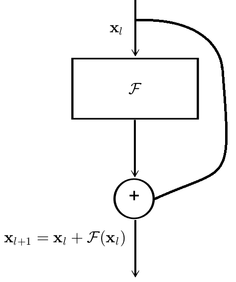
In this work, we unify the training and testing of ResNets with the theory of transport equations (TEs). This unified viewpoint enables us to interpret the adversarial vulnerability of ResNets as the irregularity, which will be defined later, of the TE’s solution. Based on this observation, we propose a new ResNets ensemble algorithm based on the Feynman-Kac formula. In a nutshell, the proposed algorithm consists of two essential components. First, for each $l=1,2,\cdots,M$ with $M$ being the number of residual mappings in the ResNet, we modify the $l$-th residual mapping from $\mathbf{x}_{l+1}=\mathbf{x}_{l}+\mathcal{F}(\mathbf{x}_{l})$ (Fig. 1 (a)) to $\mathbf{x}_{l+1}=\mathbf{x}_{l}+\mathcal{F}(\mathbf{x}_{l})+N(0,\sigma^{2}\mathbf{I})$ (Fig. 1 (b)), where $\mathbf{x}_{l}$ is the input, $\mathcal{F}$ is the residual mapping and $N(0,\sigma^{2}\mathbf{I})$ is Gaussian noise with a specially designed variance $\sigma^{2}$. Second, we average over multiple jointly and robustly trained modified ResNets’ outputs to get the final prediction (Fig. 2). This ensemble algorithm improves the base model’s accuracy on both clean and adversarial data. The advantages of the proposed algorithm are summarized as follows:

• •

  It outperforms the current state-of-the-art in defending against inference attacks.

• •

  It improves the natural accuracy of the adversarially trained models.

• •

  Its defense capability can be improved dynamically as the base ResNet advances.

• •

  It enables to train and integrate an ultra-large DNN for adversarial defense with a limited GPU memory.

• •

  It is motivated from partial differential equation (PDE) theory, which introduces a new way to defend against adversarial attacks, and it is a complement to many other existing adversarial defenses.

There is a massive volume of research over the last several years on defending against adversarial attacks for DNNs. Randomized smoothing transforms an arbitrary classifier $f$ into a "smoothed" surrogate classifier $g$ and is certifiably robust in $\ell_{2}$ norm based adversarial attacks [34, 33, 12, 54, 8]. Among the randomized smoothing, one of the most popular ideas is to inject Gaussian noise to the input image and the classification result is based on the probability of the noisy image in the decision region. Our adversarial defense algorithm injects noise into each residual mapping instead of the input image, which is different from randomized smoothing.

Robust optimization for solving EARM achieves great success in defending against inference attacks [38, 44, 45, 55, 47]. Regularization in EARM can further boost the robustness of the adversarially trained models [57, 30, 46, 60]. The adversarial defense algorithms should learn a classifier with high test accuracy on both clean and adversarial data. To achieve this goal, Zhang et al. [59] developed a new loss function, TRADES, that explicitly trades off between natural and robust generalization. To the best our of knowledge, TRADES is the current state-of-the-art in defending against inference attacks on the CIFAR10. Throughout this paper, we regard TRADES as the benchmark.

Modeling DNNs as ordinary differential equations (ODEs) has drawn lots of attention recently. Chen et al. proposed neural ODEs for DL [10]. E [14] modeled training ResNets as solving an ODE optimal control problem. Haber and Ruthotto [19] constructed stable DNN architectures based on the properties of numerical ODEs. Lu, Zhu and et al. [37, 61] constructed novel architectures for DNNs, which were motivated from the numerical discretization schemes for ODEs. Sun et al. [50] modeled training of ResNets as solving a stochastic differential equation.

Model averaging with multiple stochastically trained identical DNNs is the most straightforward ensemble technique to improve the predictive power of base DNNs. This simple averaging method has been a success in image classification for ILSVRC competitions. Different groups of researchers use model averaging for different base DNNs and won different ILSVRC competitions [29, 48, 21]. This widely used unweighted averaging ensemble, however, is not data-adaptive and is sensitive to the presence of excessively biased base learners. Ju et al., recently investigated ensemble of DNNs by many different ensemble methods, including unweighted averaging, majority voting, the Bayes Optimal Classifier, and the (discrete) Super Learner, for image recognition tasks. They concluded that the Super Learner achieves the best performance among all the studied ensemble algorithms [25].

Our work distinguishes from the existing work on DNN ensemble and feature and input smoothing from two major points: First, we inject Gaussian noise to each residual mapping in the ResNet. Second, we jointly train each component of the ensemble instead of using a sequential training.

We organize this paper in the following way: In section 2, we model the ResNet as a TE and give an explanation for ResNet’s adversarial vulnerability. In section 3, we present a new ResNet ensemble algorithm that motivated from the Feynman-Kac formula for adversarial defense. In section 4, we present the natural accuracy of the EnResNets and their robust accuracy under both white-box and blind PGD and C&W attacks, and compare with the current state-of-the-art. In section 5, we generalize the algorithm to ensemble of different neural nets and numerically verify its efficacy. Our paper ends up with some concluding remarks.

The connection between training ResNet and solving optimal control problems of the TE is investigated in [52, 53, 35]. In this section, we derive the TE model for ResNet and explain its adversarial vulnerability from a PDE viewpoint. The TE model enables us to understand the data flow of the entire training and testing data in both forward and backward propagation in training and testing of ResNets; whereas, the ODE models focus on the dynamics of individual data points [10].

As shown in Fig. 1 (a), residual mapping adds a skip connection to connect the input and output of the original mapping ($\mathcal{F}$), and the $l$-th residual mapping can be written as

with $\mathbf{x}_{0}=\hat{\mathbf{x}}\in T\subset\mathbb{R}^{d}$ being a data point in the set $T$, $\mathbf{x}_{l}$ and $\mathbf{x}_{l+1}$ are the input and output tensors of the residual mapping. The parameters $\mathbf{w}_{l}$ can be learned by back-propagating the training error. For $\forall\ \hat{\mathbf{x}}\in T$ with label $y$, the forward propagation of ResNet can be written as

where $\hat{y}$ is the predicted label, $L$ is the number of layers, and $f(\mathbf{x})={\rm softmax}(\mathbf{w}_{0}\cdot\mathbf{x})$ be the output activation with $\mathbf{w}_{0}$ being the trainable parameters. For the widely used residual mapping in the pre-activated ResNet [22], as shown in Fig. 3 (a), we have

where $\mathbf{w}_{l}^{\rm C1}(\mathbf{w}_{l}^{\rm B1})$ and $\mathbf{w}_{l}^{\rm C2}(\mathbf{w}_{l}^{\rm B2})$ are the first and second convolutional (batch normalization) layers of the $l$-th residual mapping, respectively, from top to bottom order. $\otimes$ and $\odot$ are the convolutional and batch normalization operators, respectively.

Next, we introduce a temporal partition: let $t_{l}=l/L$, for $l=0,1,\cdots,L$, with the time interval $\Delta t=1/L$. Without considering dimensional consistency, we regard $\mathbf{x}_{l}$ in Eq. (3) as the value of $\mathbf{x}(t)$ at the time slot $t_{l}$, so Eq. (3) can be rewritten as

where $\overline{F}\doteq\frac{1}{\Delta t}\mathcal{F}$. Eq. (5) is the forward Euler discretization of the following ODE

Let $u(\mathbf{x},t)$ be a function that is constant along the trajectory defined by Eq. (6), as demonstrated in Fig. 3 (b), then $u(\mathbf{x},t)$ satisfies the following TE

the first equality is because of the chain rule and the second equality dues to the fact that $u$ is constant along the curve defined by Eq. (6).

If we enforce the terminal condition at $t=1$ for Eq. (7) to be

then according to the fact that $u(\mathbf{x},t)$ is constant along the curve defined by Eq. (6) (which is called the characteristic curve for the TE defined in Eq. (7)), we have $u(\hat{\mathbf{x}},0)=u(\mathbf{x}(1),1)=f(\mathbf{x}(1))$; therefore, the forward propagation of ResNet for $\hat{\mathbf{x}}$ can be modeled as computing $u(\hat{\mathbf{x}},0)$ along the characteristic curve of the following TE

Meanwhile, the backpropagation in training ResNets can be modeled as finding the velocity field, $\overline{F}(\mathbf{x}(t),\mathbf{w}(t))$, for the following control problem

where $T$ is the training set that enforces the initial condition on the training data for the TE. Note that in the above TE formulation of ResNet, $u(\mathbf{x},0)$ serves as the classifier and the velocity field $\overline{F}(\mathbf{x},\mathbf{w}(t))$ encodes ResNet’s architecture and weights. When $\overline{F}$ is very complex, $u(\mathbf{x},0)$ might be highly irregular i.e. a small change in the input $\mathbf{x}$ can lead to a massive change in the value of $u(\mathbf{x},0)$. This irregular function may have a good generalizability on clean images, but it is not robust to adversarial attacks. Fig. 4 (a) shows a 2D illustration of $u(\mathbf{x},0)$ with the terminal condition $u(\mathbf{x},1)$ shown in Fig. 4 (d); we will discuss this in detail later in this section.

Using a specific level set of $u(\mathbf{x},0)$ in Fig. 4 (a) for classification suffers from adversarial vulnerability: A tiny perturbation in $\mathbf{x}$ will lead the output to go across the level set, thus leading to misclassification. To mitigate this issue, we introduce a diffusion term $\frac{1}{2}\sigma^{2}\Delta u$ to Eq. (8), with $\sigma$ being the diffusion coefficient and

is the Laplace operator in $\mathbb{R}^{d}$. The newly introduced diffusion term makes the level sets of the TE more regular. This improves adversarial robustness of the classifier. Hence, we arrive at the following convection-diffusion equation

The solution of Eq. (10) is much more regular when $\sigma\neq 0$ than when $\sigma=0$. We consider the solution of Eq. (10) in a 2D unit square with periodic boundary conditions, and on each grid point of the mesh the velocity field $\overline{F}(\mathbf{x},\mathbf{w}(t))$ is a random number sampled uniformly from $-1$ to $1$. The terminal condition is also randomly generated, as shown in Fig. 4 (d). This 2D convection-diffusion equation is solved by the pseudo-spectral method with spatial and temporal step sizes being $1/128$ and $1\times 10^{-3}$, respectively. Figure 4 (a), (b), and (c) illustrate the solutions when $\sigma=0$, $0.01$, and $0.1$, respectively. These show that as $\sigma$ increases, the solution becomes more regular, which makes the classifier more robust, but might be less accurate on clean data. The $\sigma$ should be selected to have a good trade-off between accuracy and robustness. According to the above observation, instead of using $u(\mathbf{x},0)$ of the TE’s solution for classification, we use that of the convection-diffusion equation.

We have the following theoretical guarantee for robustness of the solution of the convection-diffusion equation mentioned above.

Furthermore, we have the following bound for the gradient of the solution of the convection-diffusion equation.

Based on the above discussion, if we use the solution of the convection-diffusion equation, Eq. (10), for classification. The resulted classifier will be more resistant to adversarial attacks. In this part, we will present an ensemble of ResNets to approximate the solution of Eq. (10). In the Section. 4, we will verify that the robustly trained special ensemble of ResNets is more accurate on both clean and adversarial images than standard ResNets.

The convection-diffusion equation, Eq. (10), can be solved using the Feynman-Kac formula [26] in high dimensional space, which gives $u(\hat{\mathbf{x}},0)$ as

where $\mathbf{x}(t)$ is an Itô process,

and $u(\hat{\mathbf{x}},0)$ is the conditional expectation of $f(\mathbf{x}(1))$.

Next, we approximate the Feynman-Kac formula by an ensemble of modified ResNets in the following way: Accoding to the Euler-Maruyama method [2], the term $\sigma dB_{t}$ in the Itô process that can be approximated by adding a specially designed Gaussian noise, $\sigma\mathcal{N}(\mathbf{0},\mathbf{I})$, where $\sigma=a\sqrt{{\rm Var}(\mathbf{x}_{l}+\mathcal{F}(\mathbf{x}_{l}))}$ with $a$ being a tunable parameter, to each original residual mapping $\mathbf{x}_{l+1}=\mathbf{x}_{l}+\mathcal{F}(\mathbf{x}_{l})$ in the ResNet. This gives the modified residual mapping $\mathbf{x}_{l+1}=\mathbf{x}_{l}+\mathcal{F}(\mathbf{x}_{l})+\sigma\mathcal{N}(\mathbf{0},\mathbf{I})$, as illustrated in Fig. 1 (b). Let ResNet’ denote the modified ResNet where we inject noise to each residual mapping of the original ResNet. In a nutshell, ResNet’s approximation to the Feynman-Kac formula is an ensemble of jointly trained ResNet’ as illustrated in Fig. 1 (c). ¹¹ 1 To ease the notation, in what follows, we use ResNet in place of ResNet’ when there is no ambiguity. We call this ensemble of ResNets as EnResNet. For instance, if the base ResNet is ResNet20, an ensemble of $n$ ResNet20 is denoted as En_nResNet20.

In this subsection, we review a few widely used adversarial attacks. These attacks will be used to train robust EnResNets and attack the trained models. We attack the trained model, $f(\mathbf{x},\mathbf{w})$, by $\ell_{\infty}$ norm based (the other norm based attacks can be formulated similarly) untargeted fast gradient sign method (FGSM), iterative FGSM (IFGSM) [16], and Carlini-Wagner (C&W) [9] attacks in both white-box and blind fashions. In blind attacks, we use the target model to classify the adversarial images crafted by attacking the oracle model in a white-box approach. For a given instance ($\mathbf{x}$, $y$):

• •

  FGSM searches the adversarial image $\mathbf{x}^{\prime}$ by maximizing the loss function $\mathcal{L}(\mathbf{x}^{\prime},y)\doteq\mathcal{L}(f(\mathbf{x}^{\prime},\mathbf{w}),y)$, subject to the constraint $||\mathbf{x}^{\prime}-\mathbf{x}||_{\infty}\leq\epsilon$ with $\epsilon$ being the maximum perturbation. For the linearized loss function, $\mathcal{L}(\mathbf{x}^{\prime},y)\approx\mathcal{L}(\mathbf{x},y)+\nabla_{x}\mathcal{L}(\mathbf{x},y)^{T}\cdot(\mathbf{x}^{\prime}-\mathbf{x})$, the optimal adversarial is

  $$\mathbf{x}^{\prime}=\mathbf{x}+\epsilon\cdot{\rm sign}\left(\nabla_{\mathbf{x}}\mathcal{L}(\mathbf{x},y)\right).$$

  (15)

• •

  IFGSM, Eq. (16), iterates FGSM with step size $\alpha$ and clips the perturbed image to generate the enhanced adversarial attack,

  $$\mathbf{x}^{(m)}={\rm Clip}_{\mathbf{x},\epsilon}\{\mathbf{x}^{(m-1)}+\alpha\cdot{\rm sign}(\nabla_{\mathbf{x}}\mathcal{L}(\mathbf{x}^{(m-1)},y))\},$$

  (16)

  where $m=1,\cdots,M$, $\mathbf{x}^{(0)}=\mathbf{x}$, and let the adversarial image be $\mathbf{x}^{\prime}=\mathbf{x}^{(M)}$ with $M$ being the total number of iterations.

• •

  C&W attack searches the targeted adversarial image by solving

  $$\min_{\delta}||\delta||_{\infty},\ \ \mbox{subject to}\ \ f(\mathbf{w},\mathbf{x}+\delta)=t,\;\mathbf{x}+\delta\in[0,1]^{d},$$

  (17)

  where $\delta$ is the adversarial perturbation and $t$ is the target label. Carlini et al. [9] proposed the following approximation to Eq. (17),

  	$\displaystyle\min_{\mathbf{u}}||\frac{1}{2}\left(\tanh(\mathbf{u})+1\right)-\mathbf{x}||_{\infty}+$		(18)
  	$\displaystyle c\cdot\max\left\{-\kappa,\max_{i\neq t}(Z(\frac{1}{2}(\tanh(\mathbf{u}))+1)_{i})-Z(\frac{1}{2}(\tanh(\mathbf{u}))+1)_{t}\right\},$

  where $Z(\cdot)$ is the logit vector for the input, i.e., the output of the DNN before the softmax layer. This unconstrained optimization problem can be solved efficiently by using the Adam optimizer [27]. Dou et al. [13], prove that, under a certain regime, C&W can shift the DNNs’ predicted probability distribution to the desired one.

All three attacks clip the pixel values of the adversarial image to between 0 and 1. In the following experiments, we set $\epsilon=8/255$ in both FGSM and IFGSM attacks. Additionally, in IFGSM we set $m=20$ and $\alpha=2/255$, and denote it as IFGSM²⁰. For C&W attack, we run 50 iterations of Adam with learning rate $6\times 10^{-4}$ and set $c=10$ and $\kappa=0$.

We use the PGD adversarial training [38], i.e., solving EARM Eq. (1) by replacing $\mathbf{x}^{\prime}$ with the PGD adversarial one, to robustly train EnResNets with $\sigma=0.1$ on both CIFAR10 and CIFAR100 [28] benchmarks with standard data augmentation [21]. The attack in the PGD adversarial training is merely IFGSM with an initial random perturbation on the clean data. We summarize the PGD based robust training for EnResNets in Algorithm 1. Other methods to solve EARM can also be used to train EnResNets, e.g., approximation to the adversarial risk function and regularization. EnResNet enriches the hypothesis class $\mathcal{H}$, to make the classifiers from $\mathcal{H}$ more adversarially robust. All computations are carried out on a machine with a single Nvidia Titan Xp graphics card.

In robust training, we run 200 epochs of the PGD adversarial training (10 iterations of IFGSM with $\alpha=2/255$ and $\epsilon=8/255$, and an initial random perturbation of magnitude $\epsilon$) with initial learning rate $0.1$, which decays by a factor of $10$ at the 80th, 120th, and 160th epochs. The training data is split into 45K/5K for training and validation, the model with the best validation accuracy is used for testing. Similar settings are used for natural training, i.e., solving the ERM problem Eq. (2). En₁ResNet20 denotes the ensemble of only one ResNet20 which is merely adding noise to each residual mapping, and similar notations apply to other DNNs.

First, we show that the ensemble of noise injected ResNets can improve the natural generalization of the naturally trained models. As shown in Table 1, the naturally trained ensemble of multiple ResNets are always generalize better on the clean images than the base ResNets. This conclusion is verified by ResNet20, ResNet44, and ResNet110. However, the natural accuracy of the robustly trained models are much less than that of the naturally trained models. For instance, the natural accuracies of the robustly trained and naturally trained ResNet20 are, respectively, $75.11$% and $92.10$%. The degradation of natural accuracies in robust training are also confirmed by experiments on ResNet44 ($78.89$% v.s. $93.22$%) and ResNet110 ($82.19$% v.s. $94.30$%). Improving natural accuracy of the robustly trained models is another important issue during adversarial defense.

Second, consider natural ($\mathcal{A}_{\rm nat}$) and robust ($\mathcal{A}_{\rm rob}$) accuracies of the PGD adversarially trained models on the CIFAR10, where $\mathcal{A}_{\rm nat}$ and $\mathcal{A}_{\rm rob}$ are measured on clean and adversarial images, respectively. All results are listed in Table 2. The robustly trained ResNet20 has accuracies $50.89$%, $46.03$% (close to that reported in [38]), and $58.73$%, respectively, under the FGSM, IFGSM²⁰, and C&W attacks. Moreover, it has a natural accuracy of $75.11$%. En₅ResNet20 boosts natural accuracy to $82.52$%, and improves the corresponding robust accuracies to $58.92$%, $51.48$%, and $67.73$%, respectively. Simply injecting noise to each residual mapping of ResNet20 can increase $\mathcal{A}_{\rm nat}$ by $\sim 2\%$ and $\mathcal{A}_{\rm rob}$ by $\sim 3\%$ under the IFGSM²⁰ attack. The advantages of EnResNets are also verified by experiments on ResNet44, ResNet110, and their ensembles. Note that ensemble of high capacity ResNet is more robust than low capacity model: as shown in Table 2, En₂ResNet110 is more accurate than En₂ResNet44 which in turn is more accurate than En₂ResNet20 in classifying both clean and adversarial images. The robustly trained En₁WideResNet34-10 has $86.19$% and $56.60$%, respectively, natural and robust accuracies under the IFGSM²⁰ attack. Compared with the current state-of-the-art [59], En₁WideResNet34-10 has almost the same robust accuracy ($56.60\%$ v.s. $56.61\%$) under the IFGSM²⁰ attack but better natural accuracy ($86.19\%$ v.s. $84.92\%$). Figure 5 plots the evolution of training and validation accuracies of ResNet20 and ResNet44 and their different ensembles.

Third, consider accuracy of the robustly trained models under blind attacks. In this scenario, we use the target model to classify the adversarial images crafted by applying FGSM, IFGSM²⁰, and C&W attacks to the oracle model. As listed in Table 3, EnResNets are always more robust than the base ResNets under different blind attacks. For instance, when En₅ResNet20 is used to classify adversarial images crafted by attacking ResNet20 with FGSM, IFGSM²⁰, and C&W attacks, the accuracies are $64.07$%, $62.99$%, and $76.57$%, respectively. Conversely, the accuracies of ResNet20 are only $61.69$%, $58.74$%, and $73.77$%, respectively, in classifying adversarial images obtained by using the above three attacks to attack En₅ResNet20.

Fourth, we perform experiments on the CIFAR100 to further verify the efficiency of EnResNets in defending against adversarial attacks. Table 4 lists the naturally accuracies of the naturally trained ResNets and their ensembles, again, the ensemble can improve natural accuracies. Table 5 lists natural and robust accuracies of robustly trained ResNet20, ResNet44, and their ensembles under white-box attacks. The robust accuracy under the blind attacks is listed in Table 6. The natural accuracy of the PGD adversarially trained baseline ResNet20 is $46.02$%, and it has robust accuracies $24.77$%, $23.23$%, and $32.42$% under FGSM, IFGSM²⁰, and C&W attacks, respectively. En₅ResNet20 increases them to $51.72$%, $31.64$%, $27.80$%, and $40.44$%, respectively. The ensemble of ResNets is more effective in defending against adversarial attacks than making the ResNets deeper. For instance, En₂ResNet20 that has $\sim 0.27M\times 2$ parameters is much more robust to adversarial attacks, FGSM ($30.20$% v.s. $28.40$%), IFGSM²⁰ ($26.25$% v.s. $25.81$%), and C&W ($40.06$% v.s. $36.06$%), than ResNet44 with $\sim 0.66M$ parameters. Under blind attacks, En₂ResNet20 is also significantly more robust to different attacks where the opponent model is used to generate adversarial images. Under the same model and computation complexity, EnResNets is more robust to adversarial images and more accurate on clean images than deeper nets.

Figure 6 depicts a few selected images from the CIFAR10 and their adversarial ones crafted by applying either IFGSM²⁰ or C&W attack to attack both ResNet20 and En₅ResNet20. Both adversarially trained ResNet20 and En₅ResNet20 fail to correctly classify any of the adversarial versions of these four images. For the deer image, it might also be difficult for human to distinguish it from a horse.

In the previous subsection, we verified the adversarial defense capability of EnResNet, which is an approximation to the Feynman-Kac formula to solve the convection-diffusion equation. As we showed, when more ResNets and larger models are involved in the ensemble, both natural and robust accuracies are improved. However, EnResNet proposed above requires to train the ensemble jointly, which poses memory challenges for training ultra-large ensembles. To overcome this issue, we consider training each component of the ensemble individually and integrating them together for prediction. The major benefit of this strategy is that with the same amount of GPU memory, we can train a much larger model for inference since the batch size used in inference can be one.

Table 7 lists natural and robust accuracies of the integration of separately trained EnResNets on the CIFAR10. The integration of separately trained EnResNets have better robust accuracy than each component. For instance, the integration of En₂ResNet110 and En₁WideResNet34-10 gives a robust accuracy ${\bf 57.94}$% under the IFGSM²⁰ attack, which is remarkably better than both En₂ResNet110 ($53.05$%) and En₁WideResNet34-10 ($56.60$%). To the best of our knowledge, $57.94$% outperforms the current state-of-the-art [59] by $1.33$%. The effectiveness of the integration of separately trained EnResNets sheds light on the development of ultra-large models to improve efficiency for adversarial defense.

In this subsection, we show that with the same number of parameters, EnResNets is more adversarially robust that the Wide ResNets. We compare EnResNet₂20 with the wide-ResNet: WRN-14-2 [58]. WRN-14-2 has $\sim 0.69$M parameters which is more than that of EnResNet₂20. We list natural and robust accuracies of the robustly trained models on the CIFAR10 benchmark in Table. 8. En₂ResNet20 has higher natural accuracy than WRN-14-2 ($80.34$% v.s. $78.37$%). Moreover, En₂ResNet20 is more robust to both IFGSM²⁰ and C&W attacks.

Besides applying EOT gradient, we further verify that our defense is not due to obfuscated gradient. We use IFGSM²⁰ to attack naturally trained (using the same approach as that used in [21]) En₁ResNet20, En₂ResNet20, and En₅ResNet20, and the corresponding accuracies are: $0$%, $0.02$%, and $0.03$%, respectively. All naturally trained EnResNets are easily fooled by IFGSM²⁰, thus gradient mask does not play an important role in EnResNets for adversarial defense [5].

Ensemble of models for adversarial defense has been studied in [49]. Here, we show that ensembles of robustly trained ResNets without noise injection cannot boost natural and robust accuracy much. The natural accuracy of jointly (separately) adversarially trained ensemble of two ResNet20 without noise injection is $75.75$% ($74.96$%), which does not substantially outperform ResNet20 with a natural accuracy $75.11$%. The corresponding robust accuracies are $51.11$% ($51.68$%), $47.28$% ($47.86$%), and $59.73$% ($59.80$%), respectively, under the FGSM, IFGSM²⁰, and C&W attacks. These robust accuracies are much inferior to that of En₂ResNet20. Furthermore, the ensemble of separately trained robust ResNet20 and robust ResNet44 gives a natural accuracy of $77.92$%, and robust accuracies are $54.73$%, $51.47$%, $61.77$% under the above three attacks. These results reveal that ensemble adversarially trained ResNets via the Feynman-Kac formalism is much more accurate than standard ensemble in both natural and robust generalizations.

References

- [1] Adversarial machine learning against Tesla’s autopilot. https://www.schneier.com/blog/archives/2019/04/adversarial_mac.html.
- [2] P. Kloeden abd E. Platen. Numerical Solution of Stochastic Differential Equations. Springer, 1992.
- [3] N. Akhtar and A. Mian. Threat of adversarial attacks on deep learning in computer vision: A survey. arXiv preprint arXiv:1801.00553, 2018.
- [4] Naveed Akhtar, Jian Liu, and Ajmal Mian. Defense against universal adversarial perturbations. In The IEEE Conference on Computer Vision and Pattern Recognition (CVPR), June 2018.
- [5] A. Athalye, N. Carlini, and D. Wagner. Obfuscated gradients give a false sense of security: Circumventing defenses to adversarial examples. International Conference on Machine Learning, 2018.
- [6] A. Athalye, L. Engstrom, A. Ilyas, and K. Kwok. Synthesizing robust adversarial examples. International Conference on Machine Learning, 2018.
- [7] W. Brendel, J. Rauber, and M. Bethge. Decision-based adversarial attacks: Reliable attacks against black-box machine learning models. arXiv preprint arXiv:1712.04248, 2017.
- [8] X. Cao and N. Gong. Mitigating evasion attacks to deep neural networks via region-based classification. In 33rd Annual Computer Security Applications Conference, 2017.
- [9] N. Carlini and D.A. Wagner. Towards evaluating the robustness of neural networks. IEEE European Symposium on Security and Privacy, pages 39–57, 2016.
- [10] R. Chen, Y. Rubanova, J. Bettencourt, and D. Duvenaud. Neural ordinary differential equations. In Advances in Neural Information Processing Systems, 2018.
- [11] X. Chen, C. Liu, B. Li, K. Liu, and D. Song. Targeted backdoor attacks on deep learning systems using data poisoning. arXiv preprint arXiv:1712.05526, 2017.
- [12] J. Cohen, E. Rosenfeld, and J.Z. Kolter. Certified adversarial robustness via randomized smoothing. arXiv preprint arXiv:1902.02918v1, 2019.
- [13] Z. Dou, S. J. Osher, and B. Wang. Mathematical analysis of adversarial attacks. arXiv preprint arXiv:1811.06492, 2018.
- [14] W. E. A proposal on machine learning via dynamical systems. Communications in Mathematics and Statistics, 5:1–11, 2017.
- [15] M. Giles. Multilevel monte carlo methods. Acta Numerica, pages 1–70, 2018.
- [16] I. J. Goodfellow, J. Shlens, and C. Szegedy. Explaining and harnessing adversarial examples. arXiv preprint arXiv:1412.6275, 2014.
- [17] K. Grosse, N. Papernot, P. Manoharan, M. Backes, and P. McDaniel. Adversarial perturbations against deep neural networks for malware classification. arXiv preprint arXiv:1606.04435, 2016.
- [18] A. Guisti, J. Guzzi, D.C. Ciresan, F.L. He, J.P. Rodriguez, F. Fontana, M. Faessler, C. Forster, J. Schmidhuber, G. Di Carlo, and et al. A machine learning approach to visual perception of forecast trails for mobile robots. IEEE Robotics and Automation Letters, pages 661–667, 2016.
- [19] E. Haber and L. Ruthotto. Stable architectures for deep neural networks. Inverse Problems, 34:014004, 2017.
- [20] K. L. Hansen and P. Salamon. Neural network ensembles. IEEE Transactions on Pattern Analysis and Machine Intelligence archive, pages 993–1001, 1990.
- [21] K. He, X. Zhang, S. Ren, and J. Sun. Deep residual learning for image recognition. In CVPR, pages 770–778, 2016.
- [22] K. He, X. Zhang, S. Ren, and J. Sun. Identity mappings in deep residual networks. In ECCV, 2016.
- [23] G. Huang, Z. Liu, L. van der Maaten, and K. Weinberger. Densely connected convolutional networks. In CVPR, 2017.
- [24] A. Ilyas, L. Engstrom, A. Athalye, and J. Lin. Black-box adversarial attacks with limited queries and information. International Conference on Machine Learning, 2018.
- [25] C. Ju, A. Bibaut, and M. J. van der Laan. The relative performance of ensemble methods with deep convolutional neural networks or image classification. arXiv preprint arXiv:1607.02533, 2016.
- [26] M. Kac. On distributions of certain Wiener functionals. Transactions of the American Mathematical Society, 65:1–13, 1949.
- [27] D. Kingma and J. Ba. Adam: A method for stochastic optimization. arXiv preprint arXiv:1412.6980, 2014.
- [28] A. Krizhevsky. Learning multiple layers of features from tiny images. 2009.
- [29] A. Krizhevsky, I. Sutskever, and G. E. Hinton. Imagenet classification with deep convolutional neural networks. In Advances in neural information processing systems, 2012.
- [30] A. Kurakin, I. Goodfellow, and S. Bengio. Adversarial machine learning at scale. In International Conference on Learning Representations, 2017.
- [31] O. Ladyzhenskaja, V. Solonnikov, and N. Uraltseva. Linear and Quasilinear Equations of Parabolic Type. American Mathematical Society, Providence, R.I., 1968.
- [32] Y. LeCun, Y. Bengio, and G. Hinton. Deep learning. Nature, 521:436–444, 2015.
- [33] M. Lecuyer, V. Atlidakis, R. Geambasu, D. Hsu, and S. Jana. Certified robustness to adversarial examples with differential privacy. In IEEE Symposium on Security and Privacy (SP), 2019.
- [34] B. Li, C. Chen, W. Wang, and L. Carin. Second-order adversarial attack and certifiable robustness. arXiv preprint arXiv:1809.03113, 2018.
- [35] Z. Li and Z. Shi. Deep residual learning and pdes on manifold. arXiv preprint arXiv:1708:05115, 2017.
- [36] Y. Liu, X. Chen, C. Liu, and D. Song. Delving into transferable adversarial examples and black-box attacks. arXiv preprint arXiv:1611.02770, 2016.
- [37] Y. Lu, A. Zhong, Q. Li, and Bin Dong. Beyond finite layer neural networks: Bridging deep architectures and numerical differential equations. International Conference on Machine Learning, 2018.
- [38] A. Madry, A. Makelov, L. Schmidt, D. Tsipras, and A. Vladu. Towards deep learning models resistant to adversarial attacks. In International Conference on Learning Representations, 2018.
- [39] Seyed-Mohsen Moosavi-Dezfooli, Alhussein Fawzi, Omar Fawzi, and Pascal Frossard. Universal adversarial perturbations. In The IEEE Conference on Computer Vision and Pattern Recognition (CVPR), July 2017.
- [40] Taesik Na, Jong Hwan Ko, and Saibal Mukhopadhyay. Cascade adversarial machine learning regularized with a unified embedding. In International Conference on Learning Representations, 2018.
- [41] N. Papernot, P. McDaniel, S. Jha, M. Fredrikson, Z.B. Celik, and A. Swami. The limitations of deep learning in adversarial settings. IEEE European Symposium on Security and Privacy, pages 372–387, 2016.
- [42] N. Papernot, P. McDaniel, A. Sinha, and M. Wellman. Sok: Towards the science of security and privacy in machien learning. arXiv preprint arXiv:1611.03814, 2016.
- [43] Nicolas Papernot, Patrick D. McDaniel, and Ian J. Goodfellow. Transferability in machine learning: from phenomena to black-box attacks using adversarial samples. CoRR, abs/1605.07277, 2016.
- [44] A. Raghunathan, J. Steinhardt, and P. Liang. Certified defenses against adversarial examples. In International Conference on Learning Representations, 2018.
- [45] A. Raghunathan, J. Steinhardt, and P. Liang. Semidefinite relaxations for certifying robustness to adversarial examples. In Advances in Neural Information Processing Systems, 2018.
- [46] A. Ross and F. Doshi-Velez. Improving the adversarial robustness and interpretability of deep neural networks by regularizing their input gradients. arXiv preprint arXiv:1711.09404, 2017.
- [47] H. Salman, G. Yang, H. Zhang, C. Hsieh, and P. Zhang. A convex relaxation barrier to tight robustness verification of neural networks. arXiv preprint arXiv:1902.08722, 2019.
- [48] K. Simonyan and A. Zisserman. Very deep convolutional networks for large-scale image recognition. arXiv preprint arXiv:1409.1556, 2014.
- [49] T. Strauss, M. Hanselmann, A. Junginger, and H. Ulmer. Ensemble methods as a defense to adversarial perturbations against deep neural networks. arXiv preprint arXiv:1709.0342, 2017.
- [50] Q. Sun, Y. Tao, and Q. Du. Stochastic training of residual networks: a differential equation viewpoint. arXiv preprint arXiv:1812.00174, 2018.
- [51] C. Szegedy, W. Zaremba, I. Sutskever, J. Bruna, D. Erhan, I. Goodfellow, and R. Fergus. Intriguing properties of neural networks. arXiv preprint arXiv:1312.6199, 2013.
- [52] B. Wang, A. T. Lin, Z. Shi, W. Zhu, P. Yin, A. L. Bertozzi, and S. J. Osher. Adversarial defense via data dependent activation function and total variation minimization. arXiv preprint arXiv:1809.08516, 2018.
- [53] B. Wang, X. Luo, Z. Li, W. Zhu, Z. Shi, and S. Osher. Deep neural nets with interpolating function as output activation. Advances in Neural Information Processing Systems, 2018.
- [54] E. Wong and J. Kolter. Provable defenses against adversarial examples via the convex outer adversarial polytope. In International Conference on Machine Learning, 2018.
- [55] E. Wong, F. Schmidt, J. Metzen, and J. Kolter. Scaling provable adversarial defenses. In Advances in Neural Information Processing Systems, 2018.
- [56] S. Xie, R. Girshick, P. Dollar, Z. Tu, and K. He. Aggregated residual transformations for deep neural networks. In CVPR, 2017.
- [57] D. Yin, K. Ramchandran, and P. Bartlett. Rademacher complexity for adversarially robust generalization. arXiv preprint arXiv:1810.11914, 2018.
- [58] Sergey Zagoruyko and Nikos Komodakis. Wide residual networks. In BMVC, 2016.
- [59] H. Zhang, Y. Yu, J. Jiao, E. Xing, L. Ghaoui, and M. Jordan. Theoretically principled trade-off between robustness and accuracy. arXiv preprint arXiv:1901.08573, 2019.
- [60] S. Zheng, Y. Song, T. Leung, and I. Goodfellow. Improving the robustness of deep neural networks via stability training. In IEEE Conference on Computer Vision and Pattern Recognition, 2016.
- [61] M. Zhu, B. Chang, and C. Fu. Convolutional neural networks combined with runge-kutta methods. arXiv preprint arXiv:1802.08831, 2018.