Modular decomposition of graphs and hierarchical modeling

As mentioned, the literature of MD for graph analysis is scarce. A notable exception is given in [9]. The authors in this article apply MD to help understand the structure within and between detected regions of the protein interaction network displaying 221 interactions involving 131 proteins of the human TNF-$\alpha$/NFkB signal transduction pathway. Their findings include a prime root (with 5 children), followed by parallel and series structures. A thorough biological based analysis of functional equivalence of studied units suggests that series modules can be thought of as functional single subunits, whereas parallel modules can be interpreted as alternative structures (functional equivalence) [9], pg. 10.

We consider four examples of natural networks and the Zachary Karate club graph [30] as a (small) example of a social network. The first natural network, corresponds to the transcription factor-gene interaction network of Escherichia coli from    http://regulondb.ccg.unam.mx/menu/download /datasets/index.jsp ([5]). The nodes of the network are Transcription Factors (TF), understanding that TF can regulate their own transcription. Edges indicate the existence of regulation, where the regulatory effect of the TF can be (+) activator, (-) repressor, (+-) dual or (?) unknown. All loops are eliminated.

For all networks the MD tree was obtained as well as general statistics related to the MD tree such as prime, series and parallel densities, number of levels and length of longest prime as a proxy of prime complexity.

The Zachary graph along with its MD tree and the graph of its largest prime are shown in Figure 4. Its MD tree has 3 internal nodes and 2 levels. The root of the tree is prime, followed by two parallel nodes. The prime has 29 nodes (out of 34). And the parallel nodes have, respectively 5 children (nodes 15,16,19,21 and 23 in the original graph) and 2 children (nodes 18 and 22 in the original graph). The size 5 node connects to nodes 33 and 34 and the size 2 node connects to nodes 1 and 2 in the original graph. All members of the parallel nodes established equivalent relationships with the overall group, although they do not communicate among them. The strategy of connecting to nodes 1 and 2 or to nodes 33 and 34 is repeated by the children of the parallel nodes. In particular, looking at the subgraph generated by the prime root node (right in Figure 4), the connecting role of node 1 is more clearly appreciated than in the original graph. It is interesting that vertices 1 and 34 correspond to the figures of instructor and administrator, respectively, which were the leaders around which the karate club eventually split [30].

The MD tree of the Escherichia coli transcription factor-gene interaction network has 303 internal nodes and 6 levels. This example is interesting because of the size of the original graph with 1827 nodes and 4.1K edges. Its first level is a parallel node with 23 children (connected components). Of these children two are prime, with respectively 4 and 554 children, and the rest are series or leaves. The prime nodes have parallel or series children, generally with fewer children themselves. Table 2 shows the overall statistics indicating almost 8 times as much parallel nodes as series nodes. In average series nodes have 2.05 children, whereas parallel have 5.7. Series nodes appear at level 2 and 4 and then have parallel children. Prime nodes do not have prime children. In the interpretation of section 2 ([9]), series nodes represent functional units and parallel nodes alternative structures. Recall all children of a parallel node have exactly the same connections out of the node, but do not communicate among them. Figures are not included because the number of nodes does not allow for an easy interpretation of the resulting MD tree or the original graph.

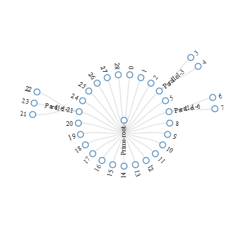
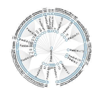
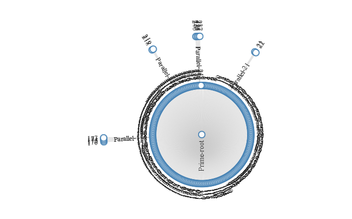
In the next examples, the three brain associated networks for different species ([2],[25]) show the same overall behavior [19]: a complex first level prime along with parallel nodes and a 3 level network in each case (see Figure 5 for the resemblance of the overall structure).Statistics for these networks are given in Table 2. Series nodes are absent and the only prime node to occur in the MD tree is the root.

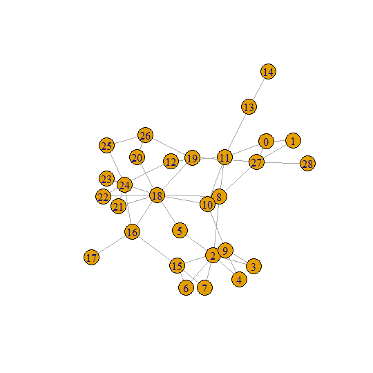
In the case of the Visual cortex mouse 1 [2], because of the small size of the original graph with 29 nodes and 44 edges it is possible to look at the MD tree in more detail as was done with Zachary social network example. Figure 6 compares the original graph to the subgraph generated by the prime root node in the MD tree. In the original graph, nodes 3 and 4 connect to nodes 2 and 9, nodes 6 and 7 connect to nodes 2 and 15. Finally, nodes 21, 22 and 23 connect to nodes 18 and 24. Connections to nodes 2,9,15, 18 and 24 are repeated by the children of the parallel nodes. The role of node 2 is especially interesting as connections to this node repeat in two different parallel children of the root.

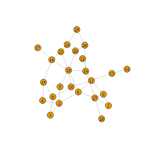This short analysis of the MD tree structure of some selected natural and social graphs, suggests that in general, prime nodes are more probable than complete nodes for connected graphs with a medium to big number of vertices. As the number of vertices decreases series and parallel nodes appear and prime nodes are less probable at the lower levels of the tree. In general, series nodes tend to have a small number of children. Understanding the behavior of the prime root node when it occurs, seems to be an important issue in describing graph behavior, as well as which children in this prime are parallel or series, and which subgraphs in the original graph are involved. Of course, more studies are required in this direction.

We consider simulations of Erdös-Renyi (ER) graphs with $n=50$ vertices and varying link-probabilities and Barabási-Albert (BA) graphs with $n=50$ vertices and “bag” method using package Igraph in R (Erdös & Renyi [7], [1] and [8], Chapter 11, for a comprehensive review on random graphs). Mean values and standard deviations for the stated statistics calculated over $N=50$ simulations are presented for each case in Table 3. Results remain unchanged by increasing the number of simulations.

Analysis of the MD tree for simulations with ER and BA random graphs show that the random graph generation procedure has an important effect on the tree structure. In Figure 7 the MD trees for ER graphs with varying link probabilities are presented. ER simulations with small values of p are not connected, so the root node is parallel. But also, primes tend to be small (with 4 to 6 children) and complete nodes (with 2 children) appear often. As p increases, although typically the root is still parallel, it has a smaller number of children and a big prime node occurs at the second level (this of course is related to the giant component, see for example [8]), with much fewer total levels. For big p, the MD tree structure is just a one level tree with a prime node. Thus, smaller values of p yield a complex, larger level MD tree but with small primes. Larger values of p yield simpler tree structures but with large, very connected primes.

BA simulated graphs have an MD tree that is always a prime root node with an average of 37 children which are either parallel nodes or leaves. The number of levels was 3 across all simulations.

An example of a simulated BA graph is presented in Figure 8. The structure coincides with the patterns produced in natural graphs, that is, a prime as the root node whose children are parallel nodes or leaves. However, the tree structure of the subgraph generated by the prime root node does not resemble neither the subgraph generated by the prime root node in the Zachary MD tree nor the subgraph generated by the prime root node in the visual cortex mouse 1 MD tree.

Results in this section provide insights for the simulation of graphs based on their MD tree: combining desired probabilities for the root types and the subsequent appereance of lower level nodes. It seems reasonable to assign high probability to prime roots in connected graphs with a large number of children, followed by parallel or series nodes with fewer children. This shall be discussed in detail in the next section.

The hierarchical nature of the proposed model allows for a very interesting level-wise approximation to the global graph properties. Although precise mathematical results for the random graphs generated with Algorithm 1 are out of the scope of this article, there are several global properties which occur naturally from the definition and which we describe in what follows. We start by introducing some necessary notation and previous results:

1. 1.

   The graph is defined by the nodes $M_{j}$ arranged in the MD tree. Each node has an assigned type $T_{j}$ and a collection of $n_{j}$ vertices arranged in a random number $K_{j}$ of children. Vertices in child $k$ of node $M_{j}$ are called $V_{j,k}\subset V$. Define $V_{j}=\cup_{k}V_{j,k}$ Set $n_{j,k}=|v_{j,k}|$. By construction, $T_{j}$ and $n_{j}$ only depend on $T_{k}$ and $n_{k}$ of node $M_{k}$ if $V_{j}\subset V_{k}$ and there does not exist $V_{m}$ with $V_{j}\subset V_{m}\subset V_{k}$.

2. 2.

   Each $v\in V$ is assigned the path $\mbox{path}(v):=\{M_{j_{i}}\}_{i\geq 0}$ of nodes containing $v$ from the the root $M_{0}$ to the leaf $v$, such that $M_{j_{0}}=M_{0}$ is the first level node. Set $L(v):=|\mbox{path}(v)|$ to be the length of $\mbox{path}(v)$. The sequence ends at the node $M_{L(v)}$ for which the child that contains $v$ contains no other vertex ($v$ is leaf). We also define $K_{j}(v)$ as the child containing vertex $v$ in $M_{j}$ and $N_{j}(v)$ as the indexes of the neighbors of $K_{j}(v)$ in $M_{j}$. Clearly, $N_{j}(v)$ depends on $T_{j}.$ Set $|N_{j}(v)|$ to be the number of neighbors of $v$ at level $j$.

3. 3.

   When $\gamma=1$, allocation in children is a Multivariate Polya-Eggenberger distribution given the number of children $k$ and number of vertices $n$, with $s=1$ and $c_{j}=1,j=1,\ldots,k$ in the notation of [15], pg. 194. Thus, the marginal distribution of the number of vertices in any given child follows a Polya-Eggenberger distribution (unidimensional). Also then, the expected number of vertices in any child is $E(n_{j,k})=n_{j}/K_{j}$, the variance is $Var(n_{j,k})=n_{j}(K_{j}+n_{j})(K_{j}-1)/(K_{j}^{2}(K_{j}+1))$ and the covariance is $Cov(n_{j,k}n_{j,l})=n_{j}(n_{j}-1)/(K_{j}(K_{j}+1))$ ([15] pgs 194-195). As a consequence, adding levels can be thought of as simply adding children. Given a sequence $(K_{1},K_{2},\ldots,K_{j})$ of number of children along the path of any given vertex, the expected number of vertices in any child $k$ at level $j$ will be $n/(K_{1}+\cdots K_{j})$. Moreover, given the path $\mbox{path}(v)$, at each level $j$, vertices may be grouped in two components: $K_{j}(v)$ and $K_{j}^{c}(v)$. Let $|A|$ stand for the number of vertices in any child $A$. Since the last descendant of $\mbox{path}(v)$ has one vertex by construction, this means that $\sum_{j=1}^{L(v)}|K_{j}^{c}(v)|=n-1$ and $|K_{j}(v)|>1$ for any $j<l$. Then the event $\{L(v)=l\}$ is equal to the event $\{l=\min_{t}\sum_{j=1}^{t}|K_{j}^{c}(v)|=n-1\}$ which in turn corresponds to all ways of distributing $n-1$ balls in $l$ urns with no empty urns. Whence, $p(L(v)=l)=\left(\begin{array}[]{c}n-2\\ l-1\end{array}\right).$

With the above notation and results for $\gamma=1$ we are able to give some preliminary results regarding the behavior of some graph characteristics: namely the structure of its adjacency matrix, degree distribution, diameter and clustering coefficient.

1. 1.

   Adjacency matrix: by construction, the adjacency matrix $A:=[a_{i,j}]$ of the generated graph has an iterative block structure. Recalling a module $M$ is defined by the property that $a_{i,j}$ is constant for all $v_{i}\in M$ and $v_{j}\not\in M$, each node $M_{j}$ generates an outer graph over its $K_{j}$ children. Let $A_{1}$ be the adjacency matrix of module $M_{1}$ over its $K_{1}$ children, so that,

   $$A_{1}=\left[\begin{array}[]{ccc}0&\cdots&b_{1,K_{1}}\\ &\ddots&\\ b_{K_{1},1}&\cdots&0\end{array}\right]$$

   (4)

   where each $b_{i,j}\in\{0,1\}$ indicates whether child $V_{1,i}$ is connected or not to child $V_{1,j}$. Each $V_{1,k}$ in turn generates an adjacency matrix $A_{1,k}$ of size $n_{1,k}$. Thus using this first level decomposition, we can write

   $$A=\left[\begin{array}[]{ccc}A_{1,1}&\cdots&B_{1,K_{1}}\\ &\ddots&\\ B_{K_{1},1}&\cdots&A_{K_{1},K_{1}}\end{array}\right]$$

   (5)

   where each $B_{i,j}$ is a constant block matrix of size $n_{1,i}\times n_{1,j}$ with entries $b_{i,j}$. Iterating the above procedure for each $A_{1,k}$ yields the stated block representation. For applications such as degree calculation or triangle counting this iterative block structure gives a level-wise approximation strategy which provides interesting insight about the overall structure.

2. 2.

   Degree of a vertex and degree distribution: by construction the degree of each vertex $v$ may be defined as

   $$dg(v)=\sum_{M_{j}\in\mbox{path}(v)}\sum_{k\in N_{j}(v)}n_{j,k}.$$

   (6)

   Alternatively, equation (6) can be obtained form the block decomposition described in (5) and calculating the diagonal of $A^{2}$, using $deg(v)=A^{2}(v)$. Whence, degree distribution depends on the collection $\{n_{j,k}\}$. As described, the model assumes a multivariate linear ($\gamma=1$) and non-linear ($\gamma>1$) Polya distribution for vertices given the number $K$ of children. General results are complex. We limit our theoretical exposition to the linear case. We have the following Lemma

   Lemma 1.

   Assume a random graph is generated using Algorithm 1 with $\gamma=1$. Then,

   	$\displaystyle E(dg(v))$	$\displaystyle=$	$\displaystyle\sum_{l}P(L(v)=l)$		(7)
   		$\displaystyle\times$	$\displaystyle\sum_{j=1}^{l}\sum_{K_{1},\ldots,K_{j}}E(n_{j,k}|L(v)=l,K_{1},\ldots,K_{j})E(|N_{j}(v)|\,\,|k_{j})$
   		$\displaystyle\times$	$\displaystyle P(K_{1},\ldots,K_{j})$

   In particular, using a first level approximation,
   

   $\displaystyle E(dg(v))$

   $\displaystyle\geq$

   $\displaystyle\sum_{k}\frac{n}{k}E(|N_{1}(v)|\,\,|k)P(k)$

   (8)

   Also, the following inequality in probability holds

   $$P(dg(v)>m)>\sum_{k=m}^{n-k}P(K_{1}=k)P(|N_{1}(v)|=m|k)$$

   (9)

   And, in particular, if the number of children follows a truncated power distribution, then

   $$P(dg(v)>m)>C(\alpha)\sum_{k=m}^{K^{\prime}}k^{-\alpha}P(|N_{1}(v)|=m|k)\propto m^{-\alpha+1}$$

   (10)

   Remark 1.

   Without the constraint $L(v)=l$, $E(n_{j,k}|K_{1},\ldots,K_{j})=\frac{n}{K_{1}+\cdots+K_{j}}$, as follows by just adding new “urns”.

   Remark 2.

   Decomposing into the possible types,

   			$\displaystyle E(|N_{j}(v)|\,\,|k_{j})$
   		$\displaystyle=$	$\displaystyle K_{j}(K_{j}-1)P(series)+E(|N_{j}(v)|\,\,|k_{j},T_{j}=prime)P(prime).$

   Where $E(|N(v)|\,\,|k,T=prime)$ is actually $E(deg(v))$ for a prime graph ($l=1$ and $T_{1}=prime$). Sometimes it is interesting to allow for a big probability first level parallel module, which would lower the r.h.s of (8) and (10). For practical applications. w.l.o.g. it can be assumed that we are considering models such that $P(T_{1}=\mbox{parallel})=0$ since this amounts to modeling connected components.

   Remark 3.

   Inequality (10) holds when the number of children follows a power distribution, thus favoring existence of nodes with a large amount of children. In practice, large series nodes are highly improbable, so that the result suggests existence of big prime nodes.

   Proof: We begin with the proof of (7). From (6),

   	$\displaystyle E(dg(v))$	$\displaystyle=$	$\displaystyle E(\sum_{M_{j}\in\mbox{path}(v)}\sum_{k\in N_{j}(v)}n_{j,k})$		(11)
   		$\displaystyle=$	$\displaystyle\sum_{l}P(L(v)=l)\sum_{j=1}^{l}E(\sum_{k\in N_{j}(v)}n_{j,k}|L(v)=l)$
   		$\displaystyle=$	$\displaystyle\sum_{l}P(L(v)=l)\sum_{j=1}^{l}\sum_{K_{1},\ldots,K_{j}}P(K_{1},\ldots,K_{j})$
   		$\displaystyle\times$	$\displaystyle E(\sum_{k\in N_{j}(v)}n_{j,k}|L(v)=l,K_{1},\ldots,K_{j})$

   Now, for each $j$, and $k$, since the addition of extra levels with $K_{j}$ children each simply increases the number of urns in which to distribute the n vertices, we have $E(n_{j,k}|L(v)=l,K_{1},\ldots,K_{j})$ does not depend on $k$ or on the particular sequence $n_{j}$. On the other hand, for a given level $j$, since the number of neighbors only depends on the type $T_{j}$ and number of children $K_{j}$ and the expectation of the number of vertices in each child is independent of the number of neighbors, we have

   			$\displaystyle E(\sum_{k\in N_{j}(v)}n_{j,k}|L(v)=l,K_{1},\ldots,K_{j})$		(12)
   		$\displaystyle=$	$\displaystyle\sum_{s}P(N_{j}(v)=s|L(v)=l,K_{1},\ldots,K_{j})$
   		$\displaystyle\times$	$\displaystyle\sum_{k=1}^{s}E(n_{j,k}|L(v)=l,K_{1},\ldots,K_{j},s)$
   		$\displaystyle=$	$\displaystyle\sum_{s}P(|N_{j}(v)|=s|K_{j})sE(n_{j,k}|L(v)=l,K_{1},\ldots,K_{j})$
   		$\displaystyle=$	$\displaystyle E(|N_{j}(v)|\,\,|K_{j})E(n_{j,k}|L(v)=l,K_{1},\ldots,K_{j},s)$

   Inequality (8) then follows by setting $l=1$ and using that $E(n_{1,k}|k)=\frac{n}{k}$ For the proof of (9), we begin again with (6). The event $deg(v)\geq m$ contains the event

   $$E=\{\mbox{the first level contains $l>m$ children of which m $\in N_{1}(v)$}\}.$$

   Thus $P(deg(v)\geq m)\geq\sum_{k\geq m}P(K_{1}=k)P(|N_{1}(v)|=m|k)$. The bound in (10) follows by assuming $K$ follows a truncated power distribution. ∎

3. 3.

   Small diameter: the distance among all vertices belonging to any child of a prime or series node is at most two. On the other hand, the diameter of the subgraph defined by the vertices in any given module is that of the outer. Thus, the existence of a large node of prime or series type assures small average diameter. We have the following result

   Lemma 2.

   For any connected graph, let $K$ be the number of children of the first level

   $$E(diam)\leq 2P(series)+P(prime)*E(K)$$

   (13)

   Proof: Conditional on the fact the graph is connected, the first node must be either prime or series. In the latter, all vertices are separated by at most 2, since vertices in any one child are all connected to all vertices in another child and all children are connected. In the former, as before, all vertices in one child are separated by at most two, and if the number of children is $k$, the max distance among chidren is $k$. Thus

   	$\displaystyle E(diam)\leq$		(14)
   	$\displaystyle 2P(series)+P(prime)*\sum_{k}kP(\mbox{number of children}=k)$

   which yields the stated result. ∎

4. 4.

   Clustering coefficient (local): given a vertex $v$ its Watts-Strogatz clustering coefficient is defined as $C(v)=\frac{2t(v)}{dg(v)(dg(v)-1)}$ (for example, see [8], pg. 101), where $t(v)$ is the number of triangles vertex $v$ belongs to and $dg(v)$ is its degree. Given a level $j$, let $t_{j}(v)\subset N_{j}(v)$ denote the neighbors of $v$ which are also neighbors, and $|t_{j}(v)|$ the number of vertices in this set. By construction, the number of triangles for vertex $v$ is

   $$t(v)=\sum_{M_{j}\in\mbox{path}(v)}\sum_{k,l\in t_{j}(v)}n_{j,k}n_{j,l}.$$

   (15)

   Alternatively, equation (15) can be obtained from the block decomposition described in (5) and calculating the diagonal of $A^{3}$, using that $t(v)=A^{3}(v)$. Although a formal characterization of $E(C(v))$ is out of the scope of this article, some insights are possible for the Polya Urn scheme with $\gamma=1$. The following result is useful

   Lemma 3.

   Assume a random graph is generated using Algorithm 1 with $\gamma=1$. Then,

   	$\displaystyle E(t(v))$	$\displaystyle=$	$\displaystyle\sum_{l}P(L(v)=s)$		(16)
   		$\displaystyle\times$	$\displaystyle\sum_{j=1}^{s}\sum_{K_{1},\ldots,K_{j}}E(n_{j,k}n_{j,l}|j\neq l,L(v)=s,K_{1},\ldots,K_{j})$
   		$\displaystyle\times$	$\displaystyle E(|t_{j}(v)|\,\,|K_{j})P(K_{1},\ldots,K_{j})$

   Proof: it follows exactly as the proof of Lemma 1. ∎

   In the definition of $C(v)$, the product in its denominator can be calculated using equation (6). We restrict the analysis of $C(v)$ to a first level approximation, conditioning on the number of children $K_{1}$ and $n$ vertices. Let $n_{k}$ be the number of vertices in child $k$. The covariance to variance ratio of the number of vertices in the children, given $K$, is then

   $$r(n,K):=Cov(n_{k}n_{l}|K)/Var(n_{k}|K)=\frac{(n-1)K}{(K-1)(K+n)}.$$

   (17)

   The expectation of the ratio

   $$R_{1}=\frac{2\sum_{k,l\in t_{1}(v)}n_{1,k}n_{1,l}}{\sum_{k\in N_{1}(v)}n_{1,k}(n_{1,k}-1)}$$

   (18)

   can then be approximated by the ratio of the conditional expectations given the number of children of the first level as

   $$E(R_{1})\approx\sum_{k}P(K_{1}=k)\frac{2E(t_{1}|k)}{E(N_{1}|k)}r(n,k)=E_{K}\frac{2E(t_{1}|K)}{E(N_{1}|K)}r(n,K),$$

   (19)

   where $E_{K}$ stands for expectation with respect to the number of children $K$. For $T_{1}=series$, $\frac{2E(t_{1}|k)}{E(N_{1}|k)}=1$. For $T_{1}=prime$ this ratio can be also very high, but no theoretical results are available.

References

- [1] A.L. Barabasi & R. Albert. (1999) Emergence of scaling in random networks, Science, 286:509–512.
- [2] D. Bock, ET. AL. (2011) Network anatomy and in vivo physiology of visual cortical neurons. Nature, 471, pp. 177–182.
- [3] B. Bollobas & O. Riordan. (2003) Mathematical results on scale-free random graphs, in Bernholdt, S.and Schuster, H.G. (eds.), Handbook of Graph and Networks: From the Genome to the Internet, Wiley-VCH,pp. 1–32.
- [4] A. Collevecchio ET. AL. (2013) On a preferential attachment and generalized Pólya’s urn model. The Annals of Applied Probability, Vol. 23, No. 3, pp. 1219–1253.
- [5] Gama-Castro S ET. AL. (2016) ”RegulonDB version 9.0: high-level integration of gene regulation, coexpression, motif clustering and beyond.”, Nucleic Acids Res., 2016 Jan 4;44(D1):D133-43.
- [6] A. Ehrenfeucht ET. AL. (1994) An Divide and Conquer Algorithm for the Prime Tree Decomposition of Two-Structures and Modular Decomposition of graphs. Journal of Algorithms, 16:283–294.
- [7] P. Erdös & A. Renyi. (1959) A. On Random Graphs I. Publicationes Mathematicae (Debrecen). Volume, 6, pp. 290–297.
- [8] E. Estrada & P. Knight. (2015) A First Course in Network Theory. Oxford University press.
- [9] J. Gagneur ET. AL. ( 2004) Modular decomposition of protein-protein interaction networks. Genome Biology, Vol. 5, Issue 8:R57.
- [10] T. Gallai. (1967) Transitive orientabare graphen. Acta mathematica Hungarica, 18, pp.25–66.
- [11] M. Habib ET. AL. (2004) A Simple Linear-Time Modular Decomposition Algorithm for Graphs, Using Order Extension. In: Hagerup T., Katajainen J. (eds) Algorithm Theory - SWAT 2004. SWAT 2004. Lecture Notes in Computer Science, vol 3111. Springer, Berlin, Heidelberg.
- [12] M. S. Handcock, A. E. Raftery & J. M. Tantrum. (2007) Model-based clustering for social networks. J. R. Statist. Soc. A, 170, Part 2, pp. 1–22
- [13] P. Holland & S. Leinhardt. (1981) An Exponential Family of Probability Distributions for Directed Graphs. Journal of the American Statistical Association, Vol. 76, No. 373, pp. 33–50.
- [14] P. Holland et. al. (1983) Stochastic Blockmodels: First Steps. Social Networks - SOC NETWORKS. 5, pp. 109–137.
- [15] N. Johnson & S. Kotz. (1977) Urn models and their applications: An approach to modern discrete probability theory, Wiley.
- [16] Karwa, V., Pelsmajer, M. J., Petrovic, S., Stasi, D., & Wilburne, D. (2017). Statistical models for cores decomposition of an undirected random graph. Electronic Journal of Statistics, 11(1), 1949-1982.
- [17] A. Mbaya & O. Hammami. (2014) Complex systems approximate matching approach for large graphs classification optimized by NSGA-II, 2014 6th International Conference of Soft Computing and Pattern Recognition (SoCPaR), Tunis, 2014, pp. 112-117.
- [18] M. Méndez. (2015) Set Operads in Combinatorics and Computer Science. Springer Briefs in Mathematics. Springer.
- [19] M. Méndez ET. AL. (2018) Hierarchical modeling of graphs using modular decomposition. Conference Abstract: 2nd International Neuroergonomics Conference.
- [20] D. Meunier ET. AL. (2010) Modular and hierarchically modular organization of brain networks. Frontiers in Science. December 2010, Volume 4, Article 200,pp. 1–11.
- [21] R.H. Möhring & F.J. Rademacher. (1984) Substitution decomposition for discrete structures and connections with combinatorial optimization. Annals of Discrete Mathematics 19, pp. 257–356.
- [22] R.H. Möhring. (1985) Algorithmic aspects of the substitution decomposition in optimization over relations, set systems and boolean functions. Annals of Operations Research 4(1985/6) pp. 195–225.
- [23] G. Palla ET. AL. (2010) Multifractal network generator PNAS April 27, 2010. 107 (17) 7640-7645.
- [24] C. Papadopoulos & C. Voglis. (2006) Drawing Graphs Using Modular Decomposition. In: Healy P., Nikolov N.S. (eds) Graph Drawing. GD 2005. Lecture Notes in Computer Science, vol 3843. Springer, Berlin, Heidelberg.
- [25] R.A. Rossi & N.K. Ahmed. (2015) The Network Data Repository with Interactive Graph Analytics and Visualization. Proceedings of the Twenty-Ninth AAAI Conference on Artificial Intelligence. pp. 4292-4293.
- [26] M. Schweinberger & M.S. Handcock. (2015) Local dependence in random graphs: characterization, properties, and statistical inference. Journal of the Royal Statistical Society: Series B (Statistical Methodology), Volume77, Issue3, pp. 647-676.
- [27] A.E. Sizemore ET. AL. (2018) Cliques and cavities in the human connectome. J Comput Neurosci Volume 44, Issue 1, pp. 115–145.
- [28] M. Tedder ET. AL. (2008) Simpler Linear-Time Modular Decomposition Via Recursive Factorizing Permutations. In: Aceto L., Damgård I., Goldberg L.A., Halldórsson M.M., Ingólfsdóttir A., Walukiewicz I. (eds) Automata, Languages and Programming. ICALP 2008. Lecture Notes in Computer Science, vol 5125. Springer, Berlin, Heidelberg.
- [29] Wasserman, S., & Faust, K. (1994). Social network analysis: Methods and applications (Vol. 8). Cambridge University press.
- [30] Zachary, W. (1977). An Information Flow Model for Conflict and Fission in Small Group., J. Anthro. Research 33(4), 452-473