Attentive Relational Networks for Mapping Images to Scene Graphs
Abstract
Scene graph generation refers to the task of automatically mapping an image into a semantic structural graph, which requires correctly labeling each extracted object and their interaction relationships. Despite the recent success in object detection using deep learning techniques, inferring complex contextual relationships and structured graph representations from visual data remains a challenging topic. In this study, we propose a novel Attentive Relational Network that consists of two key modules with an object detection backbone to approach this problem. The first module is a semantic transformation module utilized to capture semantic embedded relation features, by translating visual features and linguistic features into a common semantic space. The other module is a graph self-attention module introduced to embed a joint graph representation through assigning various importance weights to neighboring nodes. Finally, accurate scene graphs are produced by the relation inference module to recognize all entities and the corresponding relations. We evaluate our proposed method on the widely-adopted Visual Genome Dataset, and the results demonstrate the effectiveness and superiority of our model.
1 Introduction
Visual scene understanding johnson2015image; lazebnik2006beyond; zhou2014learning is a fundamental problem in computer vision. It aims at capturing the structural information in an image including the object entities and pair-wise relationships. As is shown in Figure 1, each entity and relation should be processed with a broader context to correctly understand the image at the semantic level. During recent years, deep neural network based object detection models such as Faster R-CNN girshick2015fast; ren2017faster and YOLO redmon2016you have achieved great improvements. However, such conventional object detection approaches cannot capture and infer the relationships within an image.
Because of its ability to enrich semantic analysis and clearly describe how objects interact with each other (e.g. “a boy is riding a skateboard” in Figure 1), generating scene graphs from images plays a significant role in multiple computer vision applications, such as image retrieval johnson2015image; qi2017online, image captioning li2019know; li2017scene; yao2018exploring, visual question answering li2017vip; teney2017graph and video analysis qi2018stagnet; yuan2017temporal. The highly diverse visual appearances and the large numbers of distinct visual relations make scene graph generation a challenging task.

Previous scene graph generation methods herzig2018mapping; li2018factorizable; li2017scene; newell2017pixels; xu2017scene; yang2018graph; zellers2018neural locate and infer the visual relationship as a triplet in the form subject-predicate-object, and the predicate is a word used to link a pair of objects, e.g. boy-wearing-hat in Figure 1. There exist various kinds of relationships between two objects, including spatial positions (e.g. under, above), attributes/ prepositions (e.g. with, of), comparatives (e.g. taller, shorter) and actions/ verb (e.g. play, ride). Most of the existing works neglect the semantic relationship between the visual features and linguistic knowledge, and the intra-triplet connections.
Moreover, previous works invariably utilize conventional deep learning models such as Convolutional Neural Networks (CNN) li2018factorizable; li2017scene; newell2017pixels; yang2018graph or Recurrent Neural Networks (RNN) herzig2018mapping; xu2017scene; zellers2018neural for scene graph generation. These methods require to know the graph structure beforehand and contain computationally intensive matrix operations during approximation. In addition, most of them follow a step-by-step manner to capture the representation of nodes and edges, leading to neglect the global structure and information in whole image. Effectively extracting a whole joint graph representation to model the entire scene graph for reasoning is promising but remains an arduous problem.
To address the aforementioned issues, we propose a novel Attentive Relational Network that maps images to scene graphs. To be specific, the proposed method first adopts an object detection module to extract the location and category probability of each entity and relation. Then a semantic transformation module is introduced to translate entities and relation features as well as their linguistic representation into a common semantic space. In addition, we present a graph self-attention module to jointly embed an adaptive graph representation through measuring the importance of the relationship between neighboring nodes. Finally, a relation inference module is leveraged to classify each entity and relation by a Multi-Layer Perceptron (MLP), and to generate an accurate scene graph. Our main contributions are summarized as follows:
- •
A novel Attentive Relational Network is proposed for scene graph generation, which translates visual information to a graph-structured representation.
- •
A semantic transformation module is designed to incorporate relation features with entity features and linguistic knowledge, by simultaneously mapping word embeddings and visual features into a common space.
- •
A graph self-attention module is introduced to embed the joint graph representation by implicitly specifying different weights to different neighboring nodes.
- •
Extensive experiments on the Visual Genome Dataset verify the superior performance of the proposed method compared to the state-of-the-art methods.
2 Related Work
Scene Graph Generation. Significant efforts have been devoted to this task during recent years, which can be divided into two categories: Recurrent Neural Networks (RNN)-based methods herzig2018mapping; xu2017scene; zellers2018neural and Convolutional Neural Networks (CNN)-based approaches li2018factorizable; li2017scene; newell2017pixels; yang2018graph. Xu et al. xu2017scene employ RNNs to infer scene graphs by message passing. Zellers et al. zellers2018neural introduce motifs to capture the common substructures in scene graphs. To minimize the effect of different input factors’ order, Herzig et al. herzig2018mapping propose a permutation invariant structure prediction model. Li et al. li2017scene construct a dynamic graph to address multi tasks jointly. While Newell et al. newell2017pixels present an associative embedding technique newell2017associative for predicting graphs from pixels. Yang et al. yang2018graph propose a Graph R-CNN by utilizing graph convolutional network kipf2016semi for structure embedding. Li et al. li2018factorizable present a Factorizable Net to capture subgraph-based representations. Unlike previous work, our proposed model focuses on discovering semantic relations through jointly embedding linguistic knowledge and visual representations simultaneously.
Visual Relationship Detection. Early efforts in visual relationship detection atzmon2016learning; farhadi2010every; ramanathan2015learning; sadeghi2011recognition tend to adopt a joint model regarding the relation triplet as a unique class. The visual embedding-based approaches lu2016visual; woo2018linknet; yu2017visual; zhang2017visual; zhuang2017towards place objects in a low-dimensional relation space and integrates extra knowledge. However, these works can not learn graph structural representation, which denotes the positional and logical relationships between objects in the image. Plummer et al. plummer2017phrase combine different cues with learning weights for grounded phrase. Liang et al. liang2017deep adopt variation-structured reinforcement learning to sequentially discover object relationships. Dai et al.. dai2017detecting exploit the statistical dependencies between objects and their relationships. Recently, various studies hwangtensorize; krishna2018referring; li2017vip; peyre2017weakly; yang2018shuffle; yin2018zoom; zhang2017ppr; zhang2018grounding; zhang2017relationship propose relationship proposal networks by employing pair-wise regions for fully or weakly supervised visual relation detection. However, most of them are designed for detecting relationship one-by-one, which is inappropriate for describing the structure of the whole scene. Our proposed graph self-attention based model aims at embedding a joint graph representation to describe all relationships, and applying it for scene graph generation.
3 Proposed Approach
3.1 Overview
Problem Definition: We define the scene graph of an image as , which describes the category of each entity and semantic inter-object relationships. A set of entity bounding boxes as and their corresponding class label set , where is object categories set. The set of binary relationships between objects are referred to as . Each relationship is a triplet in a subject-predictive-object format, where a subject node , a relationship label and an object node . is the set of all predicates11 1 We also adding extra ‘bg’ referred to ‘background’, denoting there is no relationship or edge between objects..
Graph Inference: Each Scene graph comprises of a collection of bounding boxes , entity labels and relation labels . The possibility of inferring a scene graph from an image can be formulated as the following:
| (1) |
The formulation can be regarded as the factorization without independence assumptions. can be inferred by the object detection module in our model described in 3.2, while and can be inferred by the rest of modules proposed in our model.
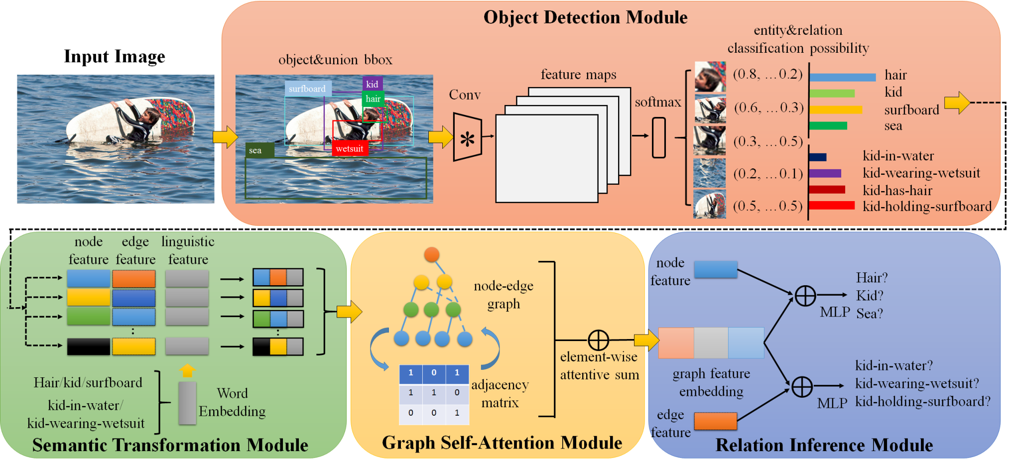
Figure 2 presents the overview of our proposed Attentive Relational Network, which contains four modules, namely object detection module, semantic transformation module, graph self-attention module and relation inference module. Our model aims at producing a joint global graph representation for the image, which contains the semantic relation translated representation learned in semantic transformation module, and the whole entity embedded representation captured in graph self-attention module. Finally, we combine the learned global graph representation and each entity/relation feature for reasoning in relation inference module. Next we will respectively introduce the four proposed modules in detail.
3.2 Object Detection Module
We employ Faster R-CNN ren2017faster as our object detector. Then a set of predictable entity proposals from each input image , including their locations and appearance features, are obtained. In order to represent the contextual information for visual relation, we generate an union bounding box to cover object pairs with a small margin. Two types of features can be adopted for describing entities and relations, i.e. the appearance feature and the spatial feature (the coordinates of the bounding box). Finally, we utilize the softmax function to recognize the category of each entity and relation, and achieve their corresponding classification confidence scores as the initial input to the following modules.
3.3 Semantic Transformation Module

Inspired by Translation Embedding (TransE) bordes2013translating; zhang2017visual and visual-semantic embedding frome2013devise, we introduce a semantic transformation module to effectively represent subject-predicate-object in the semantic domain. As depicted in Figure 3, the proposed module leverages both visual features and textual word features to learn the semantic relationship between pair-wise entities. It then explicitly maps them into a common relation space. For any relation, we define , and to represent the word embedding vectors of category labels for subject, predicate and object. To generate specific word embedding vectors for subject, predicate and object, label scores obtained from Object Detection Module and word embedding of all labels are combined with element-wise multiplication. In computational linguistics, it is known that a valid semantic relation can be expressed as the following pennington2014glove:
| (2) |
Similarly, we assume such a semantic relation exists among the corresponding visual features:
| (3) |
where , and are defined as the visual representations of entity , and their relation , respectively.
It is worth noting that the visual feature and word embedding should be projected into a common space. Hence, we adopt a linear model with three learnable weights to jointly approximate Eq. (2) and Eq. (3). L2 loss is used to guide the learning process:
| (4) |
where , and refer to the weights respectively, and denotes the concatenation operation. These learned weight matrices can be regarded as the semantic knowledge in relation space.
Then we need to map the visual features of detected entities (i.e. nodes) and relations (i.e. edges) with such linguistic knowledge into a common semantic domain. The semantic transformed representation of relation in the scene graph can be denoted as :
| (5) |
where denotes concatenation operation. Then we obtain the embedded representation of each relation in an image.
3.4 Graph Self-Attention Module

The attention mechanism maps the input to a weighted representation over the values. Especially, self-attention has been demonstrated to be effective in computing representations of a single sequence kipf2016semi; vaswani2017attention; velickovic2017graph. To compute a relational representation of a singe node sequence, we introduce a graph self-attention module that takes both node representations and their neighborhood features into consideration. By adopting the self-attention mechanism, each node’s hidden state can be extracted by attending over its neighbors and simultaneously preserve the structural relationship.
As shown in Figure 4, we define a collection of input node (entity) features , and their corresponding output features , where , and are the number of nodes, input feature dimension and output feature dimension respectively. The attention coefficients can be learned to denote the importance of node to node :
| (6) |
where denotes attention weight vector implemented with a single feed-forward layer. refers to learnable parameter weight.
We compute the for each neighboring node , where denotes the neighboring set of node . Then we normalize the coefficients across all neighboring nodes by the softmax function, for effective comparison with different nodes:
| (7) |
Therefore the coefficients computed can be formulated as:
| (8) |
where and represent Leaky ReLU nonlinear activation and concatenation operation. Final node representation is then obtained by applying the attention weights on all the neighboring node features. Inspired by vaswani2017attention, we employ multi-head attention to capture different aspect relationships from neighboring nodes. The overall output of the -th node is a concatenated feature through independent attention heads, denoted as :
| (9) |
where are normalized attention coefficients by the -th attention mechanism, refers to nonlinear function, and is the input linear transformation’s weight matrix22 2 In our experiments, we set k=8 following vaswani2017attention..
Setting of Adjacent Matrix: In order to compute adjacent matrices, we design four strategies to determine node neighbors based on spacial clues. Concretely, given two bounding boxes and as two nodes, their normalized coordinates of locations can be denoted as and , and their distance can be denoted as . Then four neighbor classification settings are: (1) Inside Neighbor: if completely includes ; (2) Cover Neighbor: if is fully covered by ; (3) Overlap Neighbor: if the IoU between and is larger than 0.5; (4) Relative Neighbor: if the ratio between the relative distance and the diagonal length of the whole images is less than 0.5.
3.5 Relation Inference Module
After obtaining the whole relation embedded representation and entity embedded representation based on Eq. (5) and Eq. (9) respectively, we can construct a global scene graph representation denoted as :
| (10) |
where refers to the number of entities in the image, and and denote element-wise sum and concatenation operation. Then we perform recognition of entity and relation with three layers MLP as the following:
| (11) |
where and refer to the predicted label of entity and relation, respectively. We adopt two cross-entropy loss functions in this module, and define and as the ground truth label for entity and relation, respectively:
| (12) |
In summary, the joint objective loss function in our Attentive Relational Network can be formulated as follows:
| (13) |
where , and denote hyper-parameters to tune the function, and refers to all learned weights in our model.
4 Experimental Results
To validate our proposed model, extensive experiments are conducted on the public Visual Genome Dataset krishna2017visual.
4.1 Experimental Settings
| Dataset | Model | SGCls | PredCls | ||
|---|---|---|---|---|---|
| Recall@50 | Recall@100 | Recall@50 | Recall@100 | ||
| VG | LP lu2016visual | 11.8 | 14.1 | 27.9 | 35.0 |
| Message Passing xu2017scene | 21.7 | 24.4 | 44.8 | 53.0 | |
| Graph R-CNN yang2018graph | 29.6 | 31.6 | 54.2 | 59.1 | |
| Neural Motif zellers2018neural | 35.8 | 36.5 | / | / | |
| GPI herzig2018mapping | 36.5 | 38.8 | / | / | |
| ST-GSA-nosemanticloss-sum | 36.6 | 38.8 | 56.4 | 60.3 | |
| ST-GSA-nosemanticloss-multiply | 34.0 | 36.8 | 53.5 | 59.7 | |
| ST-GSA-nosemanticloss-concat | 36.2 | 38.4 | 55.4 | 59.9 | |
| ST-GSA-sum | 36.9 | 39.1 | 56.6 | 61.1 | |
| ST-GSA-multiply | 36.6 | 38.4 | 56.2 | 60.7 | |
| ST-GSA-nowordembed | 37.3 | 39.8 | 55.7 | 60.6 | |
| ST-GSA-singlehead | 37.9 | 40.1 | 56.3 | 60.9 | |
| Ours w/o ST+GSA | 34.6 | 35.3 | 54.3 | 57.6 | |
| Ours w/ GSA | 37.2 | 39.4 | 54.8 | 59.9 | |
| Ours w/ ST | 37.3 | 40.1 | 55.2 | 60.9 | |
| Ours-Full | 38.2 | 40.4 | 56.6 | 61.3 | |
| Ours-Full-unconstrained | 41.4 | 46.0 | 61.6 | 68.9 | |
Visual Genome (VG) krishna2017visual includes 108,077 images annotated with bounding boxes, entities and relationships. There are 75,729 unique object categories, and 40,480 unique relationship predicates in total. Considering the effect of long-tail distribution, we choose the most frequent 150 object categories and 50 predicates for evaluation newell2017pixels; xu2017scene; zellers2018neural. For a fair comparison with previous works, we follow the experimental setting in xu2017scene, and split the dataset into 70K/5K/32K as train/validation/test sets.
Metrics: Following alexe2012measuring; lu2016visual, we adopt the image-wise Recall100 and Recall50 as our evaluation metrics. RecallX is used to compute the fraction of occurring times when the correct relationship is predicted in the top confident predictions. The rank strategy is based on confidence scores of objects and predicates. While, we do not choose as a metric, because we can not exhaustively annotate all possible relationships, and some true relationships may be missing, as discussed in lu2016visual. Besides, we also report per-type Recall5 of classifying individual predicate.
Task Settings: In this work, our goal is to infer the scene graph of an image given the confidence scores of entities and relations, while the object detection is not our main objective. Therefore, we conduct two sub-tasks of scene graph generation to evaluate our proposed method following xu2017scene; herzig2018mapping. (1)Scene Graph Classification (SGCls): Given ground truth bounding boxes of entities, the goal is to predict the category of all entities and relations in an image. This task needs to correctly detect the triplet of subject-predicate-object. (2)Predicate Classification (PredCls): Given a set of ground truth entity bounding boxes with their corresponding localization and categories, the goal is to predict all relations between entities. In all of our experiments, we perform graph-constrained evaluation, which means the returned triplets must be consistent with a scene graph. In addition, we report the results in unconstrained setting.
Compared Methods: We compare our proposed approach with the following methods on VG: Language Prior (LP) lu2016visual, Iterative Message Passing (IMP) xu2017scene, Neural Motif zellers2018neural, Graph R-CNN yang2018graph, GPI herzig2018mapping. In all experiments, the parameter settings of the above-mentioned methods are adopted from the corresponding papers. Note that some of previous methods use slightly different pre-training procedures or data split or extra supervisions. For a fair comparison, we re-train Nerual Motif and GPI with their released codes for evaluation, and ensure all the methods are based on the same backbone.
4.2 Implementation Details
We implement our model based on TensorFlow girija2016tensorflow framework on a single NVIDIA 1080 Ti GPU. Similar to prior work in scene graph generation li2017scene; xu2017scene, we adopt Faster R-CNN (with ImageNet pretrained VGG16) ren2017faster as backbone in our object detection module. Following li2017scene; xu2017scene; zellers2018neural, we adopt two-stage training, where the object detection module is pre-trained for capturing label category possibility as our high-level feature. Furthermore, the semantic transformation module is implemented as three 300-size layers for semantic projection, and one fully-connected (FC) layers for feature embedding that output a vector of size 500, and the word vectors were learned from the text data of Visual Genome with Glove pennington2014glove; the graph self-attention module is implemented by one FC layer that outputs a vector of size 500, and we set in Eq. (9) as multi-head attention; the Relation Inference Module is implemented as three FC layers of size 500 and outputs an entity probability vector of size 150 and relation probability vector of size 51 corresponding to the semantic labels in the datasets. We perform an end-to-end training by employing Adam as the optimizer with initial learning rate of , and the exponential decay rate for the 1st and 2nd moment estimates are set as and , respectively. We adopt a mini-batch training with batch size 20. The hyper-parameters in our joint loss function Eq. (12) are set as .
| predicate | ours | predicate | ours |
|---|---|---|---|
| on | 98.54 | sitting on | 80.89 |
| has | 98.18 | between | 78.62 |
| of | 96.17 | under | 66.17 |
| wearing | 99.46 | riding | 93.01 |
| in | 90.85 | in front of | 66.29 |
| near | 93.41 | standing on | 77.84 |
| with | 88.20 | walking on | 90.05 |
| behind | 88.72 | at | 73.19 |
| holding | 91.44 | attached to | 84.01 |
| wears | 95.90 | belonging to | 81.62 |
4.3 Quantitative Comparisons
As depicted in Table 1, we compare the performances of our model with the state-of-the-art methods on Visual Genome. We can see that our model outperforms all previous methods on the task of SGCls. Our full model “Ours-Full” achieves and w.r.t Recall50 and Recall100, which surpass the strong baseline method GPI by about in terms of both metrics. It indicates the superior capability of our model in capturing relations between entity pairs. Moreover, our full model also generates better performance in terms of PredCls, demonstrating our model’s ability in recognizing relationship accurately. Noting that the PredCls task is simply trying to detect predicate that requires less structural information. While our proposed semantic transformation model and graph self-attention module perform the best in jointly learning the graph structure. Compared to other similar graph-based approach, e.g. Iterative Message Passing (IMP) xu2017scene and Graph R-CNN yang2018graph, our model can capture each node’s representation by attending on the neighboring nodes to incorporate more context information and preserve the structural relationship in the image. These advantages make our model superior to xu2017scene and yang2018graph. In addition, Table 2 illustrates per-type predicate recall performances of our models on the Visual Genome test set. We find that our model achieves high Recall of over in most of the frequent predicates, as well as some less frequent ones that are harder to learn, e.g. ‘walking on’ and ‘riding’. The reason is that our framework is able to overcome the uneven relationship distribution by better modeling contextual information and diverse graph representations.
4.4 Ablation Study
In this subsection, we perform ablation studies to better examine the effectiveness of the introduced two modules.


Graph Self-Attention Module: As shown in Table 1, the graph self-attention module (“Ours w/ GSA”) brings a large improvement compared to our baseline model (“Ours w/o ST+GSA”). Moreover, our model with only graph self-attention module (“Ours w/ GSA”) outperforms Neural Motif and Graph R-CNN by and , respectively. The improvement is mainly brought by the attentive features generated from weighted neighbour embedding, which helps each node to focus on neighbor node features according to context relations. The overall module is thus able to capture more meaningful context across the entire graph and enhance the scene graph generation. In addition, we exploit the effectiveness of our proposed multi-head attention mechanism in the module. As shown in the middle part of Table 1, ours model with multi-head obtains slightly better performance than ours with single-head in terms of SGCls and PredCls, suggesting the multi-head can better capture useful information. Figure 5 illustrates an example of graph self-attention helping to generate the scene graph. Our model assigns higher attention weights on ‘ski’ to ‘man’ (0.667) and ‘snow’ to ‘man’ (0.154) than ‘mountain’ to ‘man’ (0.099), denoting the module learns to attend on more significant neighbor entities (e.g. ‘ski’ and ‘snow’). The ground truth scene graph demonstrates the detected relationships match the ground truth.

Semantic Transformation Module: As shown in Table 1, our model with only semantic transformation module (“Ours w/ ST”) outperforms all state-of-the-art results and other variants of our model, i.e. “Ours w/o ST+GSA” and “Ours w/ GSA”. This indicates the importance of the proposed semantic transformation module in generating better scene graphs. Furthermore, we examine the proposed semantic transformation loss function and different approaches of feature fusion. We introduce three variants with no semantic loss for feature fusion, i.e. concatenate (“ST-GSA-nosemanticloss-concat”), sum up (“ST-GSA-nosemanticloss-sum”) and element-wise multiply (“ST-GSA-nosemanticloss-multiply”). Moreover, we have examined other three variants with semantic loss, i.e. sum up (“ST-GSA-sum”), element-wise multiply (“ST-GSA-multiply”), visual feature only (“ST-GSA-nowordembed”). As shown in Table 1, concatenating projected features through our semantic transformation achieves the best performance, suggesting our loss function, incorporating word embedding and concatenation operation is effective and necessary. By examining the PCA visualization in a 3D space illustrated in Figure 6, we discover semantic affinities among the entity type and relation embedding of our module. Meanwhile, we notice apparent clusters of object nodes, predicate nodes and subject nodes in three dimension. Moreover, we find that the existing visual relationship can be translated into a common semantic space (denoted as orange circle in Figure 6), where the entity and relation nodes are connected in an approximate linearity, e.g. train-has-window, track-for-train and man-near-train. It demonstrates that our proposed module can learn semantic knowledge to transform visual feature and word embedding into relation space which benefits the scene graph generation tasks.
4.5 Qualitative Results
To qualitatively verify the constructed scene graph and visual relations learned by our proposed model, Figure 7 illustrates a number of visualization examples for scene graph generation on the Visual Genome dataset. The results demonstrate that our model is able to semantically predict most of visual relations in images correctly. As an example, all of visual relationships in the scene graph are correctly detected in Figure 7 (a), which has a complex structure and several different types of objects. Moreover, our model is able to resolve the ambiguity in the object-subject direction. For instance, ear-of-man and man-wearing-tie are predicted correctly by our model in Figure 7 (b). In addition, we observe that our model can predict predicates more accurately than the ground truth annotations and make more reasonable correct predictions, e.g. in Figure 7 (d) and (f) our model outputs elephant-has-leg and man-wearing-shirt, while the ground truth are elephant-on-leg and man-has-shirt that are not inappropriate for the situation. However, there are still some failure cases in our model. First, certain mistakes stem from predicate ambiguity, e.g. our model mislead in predicting bottle-above-counter and wire-hanging from-desk by bottle-on-counter and wire-on-desk in Figure 7 (f) and (e). Second, some mistakes are caused by the failure of the detector. For example, our model fails to detect any relation between ‘food’ and ‘man’ in Figure 7 (f), and some entities are detected inaccurately, e.g. ‘door’ and ‘stand’ are misled by ‘screen’ and ‘cabinet’ in Figure 7 (b), respectively. Advanced object detection model will be beneficial for improving the performance.
5 Conclusion
In this paper, we present a novel Attentive Relational Network for scene graph generation. We introduce a semantic transformation module that projects visual features and linguistic knowledge into a common space, and a graph self-attention module for joint graph representation embedding. Extensive experiments are conducted on the Visual Genome Dataset and our method outperforms the state-of-the-art methods on scene graph generation, which demonstrates the effectiveness of our model.
Acknowledgement. This work was partly supported by the National Natural Science Foundation of China (No. 61573045) and the Foundation for Innovative Research Groups through the National Natural Science Foundation of China (No. 61421003). We also would like to thank the support by NSF (Awards No.1813709, No.1704309 and No.1722847). Mengshi Qi acknowledges the financial support from the China Scholarship Council.
References
- (1) Bogdan Alexe, Thomas Deselaers, and Vittorio Ferrari. Measuring the objectness of image windows. TPAMI, 34(11):2189–2202, 2012.
- (2) Yuval Atzmon, Jonathan Berant, Vahid Kezami, Amir Globerson, and Gal Chechik. Learning to generalize to new compositions in image understanding. arXiv preprint arXiv:1608.07639, 2016.
- (3) Antoine Bordes, Nicolas Usunier, Alberto Garcia-Duran, Jason Weston, and Oksana Yakhnenko. Translating embeddings for modeling multi-relational data. In NeurlPS, 2013.
- (4) Bo Dai, Yuqi Zhang, and Dahua Lin. Detecting visual relationships with deep relational networks. In CVPR. IEEE, 2017.
- (5) Ali Farhadi, Mohsen Hejrati, Mohammad Amin Sadeghi, Peter Young, Cyrus Rashtchian, Julia Hockenmaier, and David Forsyth. Every picture tells a story: Generating sentences from images. In ECCV. Springer, 2010.
- (6) Andrea Frome, Greg S Corrado, Jon Shlens, Samy Bengio, Jeff Dean, Tomas Mikolov, et al. Devise: A deep visual-semantic embedding model. In NeurlPS, 2013.
- (7) Sanjay Surendranath Girija. Tensorflow: Large-scale machine learning on heterogeneous distributed systems. 2016.
- (8) Ross Girshick. Fast r-cnn. In ICCV. IEEE, 2015.
- (9) Roei Herzig, Moshiko Raboh, Gal Chechik, Jonathan Berant, and Amir Globerson. Mapping images to scene graphs with permutation-invariant structured prediction. In NeurlPS, 2018.
- (10) Seong Jae Hwang, Sathya N Ravi, Zirui Tao, Hyunwoo J Kim, Maxwell D Collins, and Vikas Singh. Tensorize, factorize and regularize: Robust visual relationship learning.
- (11) Justin Johnson, Ranjay Krishna, Michael Stark, Li-Jia Li, David Shamma, Michael Bernstein, and Li Fei-Fei. Image retrieval using scene graphs. In CVPR. IEEE, 2015.
- (12) Thomas N Kipf and Max Welling. Semi-supervised classification with graph convolutional networks. In ICLR, 2017.
- (13) Ranjay Krishna, Ines Chami, Michael Bernstein, and Li Fei-Fei. Referring relationships. In CVPR. IEEE, 2018.
- (14) Ranjay Krishna, Yuke Zhu, Oliver Groth, Justin Johnson, Kenji Hata, Joshua Kravitz, Stephanie Chen, Yannis Kalantidis, Li-Jia Li, David A Shamma, et al. Visual genome: Connecting language and vision using crowdsourced dense image annotations. IJCV, 123(1):32–73, 2017.
- (15) Svetlana Lazebnik, Cordelia Schmid, and Jean Ponce. Beyond bags of features: Spatial pyramid matching for recognizing natural scene categories. In CVPR. IEEE, 2006.
- (16) Xiangyang Li and Shuqiang Jiang. Know more say less: Image captioning based on scene graphs. TMM, 2019.
- (17) Yikang Li, Wanli Ouyang, and Xiaogang Wang. Vip-cnn: A visual phrase reasoning convolutional neural network for visual relationship detection. In CVPR. IEEE, 2017.
- (18) Yikang Li, Wanli Ouyang, Bolei Zhou, Jianping Shi, Chao Zhang, and Xiaogang Wang. Factorizable net: an efficient subgraph-based framework for scene graph generation. In ECCV. Springer, 2018.
- (19) Yikang Li, Wanli Ouyang, Bolei Zhou, Kun Wang, and Xiaogang Wang. Scene graph generation from objects, phrases and region captions. In ICCV. IEEE, 2017.
- (20) Xiaodan Liang, Lisa Lee, and Eric P Xing. Deep variation-structured reinforcement learning for visual relationship and attribute detection. In CVPR. IEEE, 2017.
- (21) Cewu Lu, Ranjay Krishna, Michael Bernstein, and Li Fei-Fei. Visual relationship detection with language priors. In ECCV. Springer, 2016.
- (22) Alejandro Newell and Jia Deng. Pixels to graphs by associative embedding. In NeurlPS, 2017.
- (23) Alejandro Newell, Zhiao Huang, and Jia Deng. Associative embedding: End-to-end learning for joint detection and grouping. In NeurlPS, 2017.
- (24) Jeffrey Pennington, Richard Socher, and Christopher Manning. Glove: Global vectors for word representation. In EMNLP, 2014.
- (25) Julia Peyre, Ivan Laptev, Cordelia Schmid, and Josef Sivic. Weakly-supervised learning of visual relations. In ICCV. IEEE, 2017.
- (26) Bryan A Plummer, Arun Mallya, Christopher M Cervantes, Julia Hockenmaier, and Svetlana Lazebnik. Phrase localization and visual relationship detection with comprehensive image-language cues. In CVPR. IEEE, 2017.
- (27) Mengshi Qi, Jie Qin, Annan Li, Yunhong Wang, Jiebo Luo, and Luc Van Gool. stagnet: An attentive semantic rnn for group activity recognition. In ECCV. Springer, 2018.
- (28) Mengshi Qi, Yunhong Wang, and Annan Li. Online cross-modal scene retrieval by binary representation and semantic graph. In MM. ACM, 2017.
- (29) Vignesh Ramanathan, Congcong Li, Jia Deng, Wei Han, Zhen Li, Kunlong Gu, Yang Song, Samy Bengio, Charles Rosenberg, and Li Fei-Fei. Learning semantic relationships for better action retrieval in images. In CVPR. IEEE, 2015.
- (30) Joseph Redmon, Santosh Divvala, Ross Girshick, and Ali Farhadi. You only look once: Unified, real-time object detection. In CVPR. IEEE, 2016.
- (31) Shaoqing Ren, Kaiming He, Ross Girshick, and Jian Sun. Faster r-cnn: Towards real-time object detection with region proposal networks. In NeurlPS, 2015.
- (32) Mohammad Amin Sadeghi and Ali Farhadi. Recognition using visual phrases. In CVPR. IEEE, 2011.
- (33) Damien Teney, Lingqiao Liu, and Anton van den Hengel. Graph-structured representations for visual question answering. In CVPR. IEEE, 2017.
- (34) Ashish Vaswani, Noam Shazeer, Niki Parmar, Jakob Uszkoreit, Llion Jones, Aidan N Gomez, Łukasz Kaiser, and Illia Polosukhin. Attention is all you need. In NeurlPS, 2017.
- (35) Petar Velickovic, Guillem Cucurull, Arantxa Casanova, Adriana Romero, Pietro Lio, and Yoshua Bengio. Graph attention networks. In ICLR, 2018.
- (36) Sanghyun Woo, Dahun Kim, Donghyeon Cho, and In So Kweon. Linknet: Relational embedding for scene graph. In NeurlPS, 2018.
- (37) Danfei Xu, Yuke Zhu, Christopher B Choy, and Li Fei-Fei. Scene graph generation by iterative message passing. In CVPR. IEEE, 2017.
- (38) Jianwei Yang, Jiasen Lu, Stefan Lee, Dhruv Batra, and Devi Parikh. Graph r-cnn for scene graph generation. In ECCV. Springer, 2018.
- (39) Xu Yang, Hanwang Zhang, and Jianfei Cai. Shuffle-then-assemble: learning object-agnostic visual relationship features. In ECCV. Springer, 2018.
- (40) Ting Yao, Yingwei Pan, Yehao Li, and Tao Mei. Exploring visual relationship for image captioning. In ECCV. Springer, 2018.
- (41) Guojun Yin, Lu Sheng, Bin Liu, Nenghai Yu, Xiaogang Wang, Jing Shao, and Chen Change Loy. Zoom-net: Mining deep feature interactions for visual relationship recognition. In ECCV. Springer, 2018.
- (42) Ruichi Yu, Ang Li, Vlad I Morariu, and Larry S Davis. Visual relationship detection with internal and external linguistic knowledge distillation. In ICCV. IEEE, 2017.
- (43) Yuan Yuan, Xiaodan Liang, Xiaolong Wang, Dit-Yan Yeung, and Abhinav Gupta. Temporal dynamic graph lstm for action-driven video object detection. In ICCV. IEEE, 2017.
- (44) Rowan Zellers, Mark Yatskar, Sam Thomson, and Yejin Choi. Neural motifs: Scene graph parsing with global context. In CVPR. IEEE, 2018.
- (45) Hanwang Zhang, Zawlin Kyaw, Shih-Fu Chang, and Tat-Seng Chua. Visual translation embedding network for visual relation detection. In CVPR. IEEE, 2017.
- (46) Hanwang Zhang, Zawlin Kyaw, Jinyang Yu, and Shih-Fu Chang. Ppr-fcn: weakly supervised visual relation detection via parallel pairwise r-fcn. In ICCV. IEEE, 2017.
- (47) Hanwang Zhang, Yulei Niu, and Shih-Fu Chang. Grounding referring expressions in images by variational context. In CVPR. IEEE, 2018.
- (48) Ji Zhang, Mohamed Elhoseiny, Scott Cohen, Walter Chang, and Ahmed Elgammal. Relationship proposal networks. In CVPR. IEEE, 2017.
- (49) Bolei Zhou, Agata Lapedriza, Jianxiong Xiao, Antonio Torralba, and Aude Oliva. Learning deep features for scene recognition using places database. In NeurlPS, 2014.
- (50) Bohan Zhuang, Lingqiao Liu, Chunhua Shen, and Ian Reid. Towards context-aware interaction recognition for visual relationship detection. In ICCV. IEEE, 2017.