跳到论文正文
W Papers独立论文阅读器 arXiv:1811.10513 论文正文 计算阅读时间 · 0%
引用这篇论文根据当前论文元数据生成,正式投稿前建议核对。


License: arXiv.org perpetual non-exclusive license
arXiv:1811.10513v2 [math.NA] 21 Jul 2021

Second order difference approximation for a class of Riesz space fractional advection-dispersion equations with delayJournal: Journal of Templates

M. Saedshoar Heris 1    M. Javidi Email: mo$_-$javidi@tabrizu.ac.ir Address: 1Department of Applied Mathematics, University of Tabriz, Tabriz, Iran Corresponding author: Corresponding author
Abstract

In this paper, we propose numerical scheme for the Riesz space fractional advection-dispersion equations with delay (RFADED). Firstly, analytical solution for RFADED in terms of the functions of Mittag-Leffler type is derived. Secondly, the fractional backward differential formulas (FBDF) method and shifted Grünwald method are introduced to the Riesz space fractional derivatives. Next, stability and convergency of these methods have been proved. Thirdly, Crank-Nicolson scheme for solving this problem is proposed. We prove that the scheme is conditionally stable and convergent with the order accuracy of O⁡(κ2+h2){\rm O}({\kappa^{2}}+{h^{2}}). Finally, some numerical results are given to demonstrate that presented method is a computationally efficient and accurate method for solving RFADED.

Keywords: 
Riesz fractional derivative, Fractional advection-dispersion equation with delay, Fractional backward differential formulas method, Stability and convergence.
2010 MSC
34A30, 35R11, 65L06, 65L20, 65N06.

1 Introduction

In the past few decades, fractional calculus has attracted increasing interest due to its applications in science, for examples, physics, engineering, biology, economics and finance [1, 2, 3, 4]. The fractional-order models have proved to be more accurate than integer-order models for the memory and hereditary properties of the fractional-order derivative [5, 6]. Fractional differential equations (FDEs) provide a powerful and flexible tool for modeling and describing the behavior of science such as real materials [1], fluid dynamics [3], finance, electromagnetic waves, electrochemical process [2], biological systems, control theory [7] and so on. Some numerical methods to solve the FDEs have been discussed in [8, 9, 10, 11, 12, 13]. A delay differential equation is a differential equation in which the derivative of the function at any time depends on the solution at the previous time. The fractional differential equations with delay (FDDEs) have important applications in many fields, such as, chemistry, physics, biology and finance [14]. Analytical solutions of FDDEs are complicated and hence the numerical solutions play an important role. Numerical methods for solving FDDEs are very important. For more details we refer the reader to a series of articles [15, 16, 17, 18, 19]. Partial differential equations with delays appear in many fields such as in biology, medicine, population ecology, control systems and climate models [7]. Some numerical methods for solving delay partial differential equations are studied in [20, 21, 22]. Numerical methods for solving fractional partial differential equations are investigated in [23, 24, 25].
In this paper, we consider a class of Riesz space fractional advection-dispersion equations (RFADEs)[26] with delay:

∂u⁡(x,t)∂t+Kγ​∂γu⁡(x,t−τ)∂tγ=Kα​∂αu⁡(x,t)∂|x|α+Kβ​∂βu⁡(x,t)∂|x|β+f⁡(x,t),\dfrac{{\partial u(x,t)}}{{\partial t}}+{K_{\gamma}}\dfrac{{{\partial^{\gamma}}u(x,t-\tau)}}{{\partial{{t}^{\gamma}}}}={K_{\alpha}}\dfrac{{{\partial^{\alpha}}u(x,t)}}{{\partial{{\left|x\right|}^{\alpha}}}}+{K_{\beta}}\dfrac{{{\partial^{\beta}}u(x,t)}}{{\partial{{\left|x\right|}^{\beta}}}}+f(x,t), (1)

subject to the initial condition:

u(x,t)=g(x,t),−τ≤t≤0,   0≤x≤L,u(0,t)=μ1(t),u(L,t)=μ2(t),  0≤t≤T,\begin{array}[]{l}u(x,t)=g(x,t),\,\,\,-\tau\leq t\leq 0,\,\,\,0\leq x\leq L,\\ u(0,t)={\mu_{1}}(t),\,\,u(L,t)={\mu_{2}}(t),\,\,0\leq t\leq T,\end{array} (2)

where 0<γ<1,  0<α<1,  1<β≤20<\gamma<1,\,\,0<\alpha<1,\,\,1<\beta\leq 2. uu is a solute concentration, Kα{K_{\alpha}} and Kβ{K_{\beta}} are the dispersion coefficient and the average fluid velocity, respectively. Here, we take Kα>0,Kβ≥0,Kγ≥0{K_{\alpha}>0},\,\,\,{K_{\beta}\geq 0},\,\,\,{K_{\gamma}\geq 0}. Also ff is a continuous function on [0,T]×[0,L][0,T]\times[0,L], T>0,L>0T>0,L>0 and gg is a continuous function on [−τ,0]×[0,L][-\tau,0]\times[0,L], τ>0\tau>0. The Riesz space fractional operator on a finite domain [0, L] is defined as [26]

∂ζu⁡(x,t)∂|x|ζ=−(−Δ)ζ2​u​(x,t)=−cζ​[Dxζ0R​L​u​(x,t)+DLζxR​L​u​(x,t)],\dfrac{{{\partial^{\zeta}}u(x,t)}}{{\partial{{\left|x\right|}^{\zeta}}}}=-{(-\Delta)^{\dfrac{\zeta}{2}}}u(x,t)=-{c_{\zeta}}[{}_{0}^{RL}D_{x}^{\zeta}u(x,t)+{}_{x}^{RL}D_{L}^{\zeta}u(x,t)], (3)

where

cζ=12​cos⁡(π​ζ2),    0<ζ≤2,ζ≠1.{c_{\zeta}}=\dfrac{1}{{2\cos(\frac{{\pi\zeta}}{2})}},\,\,\,\,0<\zeta\leq 2,\,\,\zeta\neq 1. (4)

Also, the left and right Riemann-Liouville derivatives of order 0<ζ≤20<\zeta\leq 2, for a given function u⁡(x,t)u(x,t) on a finite interval [0, L], are defined as [6]:

0R​LDxζu(x,t)=1Γ⁡(1−ζ)∂∂x∫0x(x−η)−ζu(η,t)dη,  0<ζ<1,xR​LDLζu(x,t)=−1Γ⁡(1−ζ)∂∂x∫xL(η−x)−ζu(η,t)dη,  0<ζ<1,0R​LDxζu(x,t)=1Γ⁡(2−ζ)∂2∂x2∫0x(x−η)1−ζu(η,t)dη,  1<ζ≤2,xR​LDLζu(x,t)=1Γ⁡(2−ζ)∂2∂x2∫xL(η−x)1−ζu(η,t)dη,  1<ζ≤2.\begin{array}[]{l}{}_{0}^{RL}D_{x}^{\zeta}u(x,t)=\dfrac{1}{{\Gamma(1-\zeta)}}\dfrac{\partial}{{\partial x}}\int\limits_{0}^{x}{{{(x-\eta)}^{-\zeta}}u(\eta,t)d\eta,}\,\,0<\zeta<1,\\ {}_{x}^{RL}D_{L}^{\zeta}u(x,t)=\dfrac{{-1}}{{\Gamma(1-\zeta)}}\dfrac{\partial}{{\partial x}}\int\limits_{x}^{L}{{{(\eta-x)}^{-\zeta}}u(\eta,t)d\eta,}\,\,0<\zeta<1,\\ {}_{0}^{RL}D_{x}^{\zeta}u(x,t)=\dfrac{1}{{\Gamma(2-\zeta)}}\dfrac{{{\partial^{2}}}}{{\partial{x^{2}}}}\int\limits_{0}^{x}{{{(x-\eta)}^{1-\zeta}}u(\eta,t)d\eta,}\,\,1<\zeta\leq 2,\\ {}_{x}^{RL}D_{L}^{\zeta}u(x,t)=\dfrac{1}{{\Gamma(2-\zeta)}}\dfrac{{{\partial^{2}}}}{{\partial{x^{2}}}}\int\limits_{x}^{L}{{{(\eta-x)}^{1-\zeta}}u(\eta,t)d\eta,}\,\,1<\zeta\leq 2.\end{array} (5)

Note that the time fractional derivative ∂γ∂tγ\dfrac{{{\partial^{\gamma}}}}{{\partial{{t}^{\gamma}}}} at the Eq (1) is the left Riemann-Liouville derivatives. Analytical and numerical solution of partial fractional differential equations (PFDEs) with delay are more complicated and less studied in the literature. The solutions of PFDEs are different from the ones for PFDEs with delay. Let us consider the case 0≤t≤τ0\leq t\leq\tau in the our model. Since −τ≤t−τ≤0-\tau\leq t-\tau\leq 0, then u⁡(x,t−τ)=g⁡(x,t−τ)u(x,t-\tau)=g(x,t-\tau) and therefore Eq (1) can be rewritten as

∂u⁡(x,t)∂t=Kα​∂αu⁡(x,t)∂|x|α+Kβ​∂βu⁡(x,t)∂|x|β+g^​(x,t),    0<t≤τ,\frac{{\partial u(x,t)}}{{\partial t}}={K_{\alpha}}\frac{{{\partial^{\alpha}}u(x,t)}}{{\partial{{\left|x\right|}^{\alpha}}}}+{K_{\beta}}\frac{{{\partial^{\beta}}u(x,t)}}{{\partial{{\left|x\right|}^{\beta}}}}+\hat{g}(x,t),\,\,\,\,0<t\leq\tau, (6)

where g^​(x,t)=f⁡(x,t)−Kγ​∂γg⁡(x,t−τ)∂tγ\hat{g}(x,t)=f(x,t)-{K_{\gamma}}\dfrac{{{\partial^{\gamma}}g(x,t-\tau)}}{{\partial{t^{\gamma}}}}. Since ff and ∂γg⁡(x,t−τ)∂tγ\dfrac{{{\partial^{\gamma}}g(x,t-\tau)}}{{\partial{t^{\gamma}}}} are continuous functions, g^​(x,t)\hat{g}(x,t) is also continuous and so (6) is solvable. Thus, we can change initial delay function to control dynamic properties of solutions.
We consider the following three fractional advection–dispersion models as the following form

  • 1.

    When Kγ=0{K_{\gamma}}=0, Eq (1) reduces to RFADE [26].

  • 2.

    When Kγ=0{K_{\gamma}}=0 and Kα=0{K_{\alpha}}=0 , Eq (1) reduces to Riesz space fractional diffusion equation(RFDE)[26].

  • 3.

    When Kγ>0{K_{\gamma}}>0, Eq (1) reduces to RFADE with delay (RFADED)
    (our main problem).

The fractional advection-dispersion equation is used in groundwater hydrology to model the transport of passive tracers carried by fluid flow in a porous medium [27, 28, 29]. At the second models, physical considerations of a fractional advection–dispersion transport model restrict 0<α<1,  1<β≤20<\alpha<1,\,\,1<\beta\leq 2 and we assume Kα>0{K_{\alpha}}>0 and Kβ≥0{K_{\beta}\geq 0} so that the flow is from left to right. The physical meaning of using homogeneous Dirichlet boundary conditions is that the boundary is set far enough away from an evolving plume such that no significant concentrations reach that boundary [30]. In this paper we consider RFADE with delay (Kγ=1{K_{\gamma}}=1).
Many models with Riesz-space fractional derivatives have recently been studied by many authors. To approximate the Riesz fractional derivative and use to numerical solving FDEs and FPDEs, there have existed several analytical and numerical methods. Zhang and Liu [31] obtained the analytical solutions of space Riesz and time Caputo fractional partial differential equations. Chen et al. [32] studied the analytical solution for the space Riesz fractional reaction dispersion equation by using the Laplace and Fourier transform. Yang et al. [26] studied the space Riesz fractional diffusion and advection–dispersion equations and solving these problems on a finite domain by using the L1, L2 methods. Later on, they [33] presented two numerical methods for solving the Riesz fractional advectiondispersion equation by using the Galerkin finite element and a backward difference methods. Shen et al. [34] used a second-order numerical scheme for the space Riesz fractional advection-dispersion equation based on fractional central difference operator. Yang et al. [26] presented three numerical methods for the space Riesz fractional diffusion and advection-dispersion equations on a finite domain. Celik and Duman [35] obtained the numerical solutions of the fractional diffusion equation with the space Riesz fractional derivative on a finite domain based on the fractional central difference operator. Recently, Ding et al. [36] constructed two different fourth-order numerical schemes for the Riesz derivative and applied to the spatial Riesz fractional diffusion equation. Later on, they [37] developed two high-order approximate schemes (sixth- and eighth-order) for the Riesz fractional derivative and use to solve the following space Riesz fractional reaction-dispersion equation. Very recently, Ding and Li [38] constructed high-order (from 2nd-order to 6th-order) numerical schemes to approximate the Riesz derivatives and develop three kinds of difference schemes for the Riesz space fractional turbulent diffusion equation. Also, Ding and Li [39] derived even-order fractional-compact numerical differential formulas for Riesz derivatives and the fourth-order formula applied to solving the Riesz spatial fractional telegraph equation. To study the long-term dynamic behaviors of these models based on Riesz derivatives, analytical solution will play a vital role. In general, since the fractional integral and fractional derivatives have non-local properties. Therefore, it seems difficult to find the analytical solution of most of these equations. Thus, it is necessary and important to design the numerical schemes to solve these equations. Other numerical methods for solving the fractional advection-dispersion equation are investigated in [40, 41, 42, 43, 36, 44, 26].
In this paper, we consider Eqs.(1-2). Firstly, we obtain analytical solution of this equation. Secondly, we use fractional backward differential formulas method of second order for 0<α<10<\alpha<1 and shifted Grünwald difference (WSGD) operators for 1<β≤21<\beta\leq 2 to approximate the Riesz space fractional derivative. Next, we obtain the Crank-Nicolson scheme by using the finite difference method for the RFADED. Also, we prove that the Crank-Nicolson scheme is conditionally stable and convergent with the accuracy O⁡(κ2+h2){\rm O}({\kappa^{2}}+{h^{2}}).
The paper is organized as follows. In Section 2, we recall some basic definitions of fractional calculus. In Section 3, analytical solution of problem is presented. Fractional backward differential formulas(FBDF) method of second order is introduced in Section 4. In Section 5, shifted Grünwald method is presented. The presented numerical method is proposed and applied to solve the Riesz space fractional advection-dispersion equations with delay (RFADED), stability and convergency of method are proved in Section 6. Finally, some numerical results are given in order to confirm the theoretical analyzes in Section 7.

2 Preliminaries

In this section, we will introduce some of the fundamental definitions. Let ℂ⁡(𝕁,ℝ)\mathbb{C(J,\mathbb{R})} denotes the Banach space of all continuous functions from 𝕁=[0,T]\mathbb{J}=[0,T] into ℝ\mathbb{R} with the norm

‖u‖∞=sup{|u⁡(t)|:t∈J},T>0.{\left\|u\right\|_{\infty}}=\sup\{\left|{u(t)}\right|:t\in J\},\,\,\,\,T>0. (7)

ℂn​(𝕁,ℝ){\mathbb{C}^{n}}(\mathbb{J},\mathbb{R}) denotes the class of all real valued functions defined on 𝕁=[0,T]\mathbb{J}=[0,T], T>0T>0 which have continuous nnth order derivatives.

Definition 2.1 ([6]). The fractional integral of order α>0\alpha>0 of the function f∈ℂ⁡(𝕁,ℝ)f\in{\mathbb{C}}(\mathbb{J},\mathbb{R}) is defined as

Iα​f​(t)=1Γ⁡(α)​∫0tf⁡(s)(t−s)1−α​𝑑s,0<t<T.{I^{\alpha}}f(t)=\frac{1}{{\Gamma(\alpha)}}\int\limits_{0}^{t}{\frac{{f(s)}}{{{{(t-s)}^{1-\alpha}}}}ds,}\,\,\,\,{\mkern 1.0mu}{\mkern 1.0mu}{\mkern 1.0mu}0<t<T. (8)

Definition 2.2 ([6]). The Caputo fractional derivative of order α>0\alpha>0 of the function f∈ℂn​(𝕁,ℝ)f\in{\mathbb{C}^{n}}(\mathbb{J},\mathbb{R}) is defined as

DαC​f​(t)={In−α​Dn​f​(t)=1Γ⁡(n−α)​∫0tf(n)​(s)(t−s)α−n+1​𝑑s,n−1<α<n,n∈N,f(n)​(t),α=n.{}^{C}{D^{\alpha}}f(t)=\left\{\begin{array}[]{l}{I^{n-\alpha}}{D^{n}}f(t)=\frac{1}{{\Gamma(n-\alpha)}}\int\limits_{0}^{t}{\frac{{{f^{(n)}}(s)}}{{{{(t-s)}^{\alpha-n+1}}}}ds,}\\ \,\,\,\,\,\,\,\,\,\,\,\,\,\,\,\,\,\,\,\,\,\,\,\,\,\,\,\,\,\,\,\,\,\,\,\,\,\,\,\,\,\,\,\,\,\,\,\,\,\,\,\,\,\,\,\,\,\,n-1<\alpha<n,\,\,n\in N,\\ {f^{(n)}}(t),\,\,\,\,\,\,\,\,\,\,\,\,\,\,\,\,\,\,\,\,\,\,\,\,\,\,\,\,\,\,\,\,\,\,\,\,\,\,\,\,\,\,\,\,\,\,\,\,\,\,\,\,\,\,\,\,\,\,\,\,\,\,\,\,\,\,\,\alpha=n.\end{array}\right. (9)

Definition 2.3 ([6, 26]). The Riesz space fractional operator of order α>0\alpha>0 of the function f∈ℂn​(𝕁,ℝ)f\in{\mathbb{C}^{n}}(\mathbb{J},\mathbb{R}) on a finite domain [0, L] is defined as

∂ζf⁡(x)∂|x|ζ=−(−Δ)ζ2​f​(x)=−cζ​[Dxζ0R​L​f​(x)+DLζxR​L​f​(x)],\frac{{{\partial^{\zeta}}f(x)}}{{\partial{{\left|x\right|}^{\zeta}}}}=-{(-\Delta)^{\frac{\zeta}{2}}}f(x)=-{c_{\zeta}}[{}_{0}^{RL}D_{x}^{\zeta}f(x)+{}_{x}^{RL}D_{L}^{\zeta}f(x)], (10)

where

cζ=12​cos⁡(π​ζ2),    0<ζ≤2,ζ≠1{c_{\zeta}}=\frac{1}{{2\cos(\frac{{\pi\zeta}}{2})}},\,\,\,\,0<\zeta\leq 2,\,\,\zeta\neq 1 (11)

Definition 2.4 ([6]). Mittag-leffler functions defined by

Eα,β​(x)=∑k=0∞xkΓ⁡(α​k+β),x,β∈ℂ,R​e​(α)>0,Eα​(x)=Eα,1.E_{\alpha,\beta}(x)=\sum\limits_{k=0}^{\infty}{\frac{{x^{k}}}{{\Gamma(\alpha k+\beta)}}}\,\,,\,\,\,x,\beta\in\mathbb{C},Re(\alpha)>0,\hfill\\ E_{\alpha}(x)=E_{\alpha,1}. (12)

Definition 2.5 ([18]). The generalized delay exponential function (of Mittag–Leffler type) is given by

Gα,βλ,τ,m​(t)=∑j=0∞(j+mj)​λj​(t−(m+j)​τ)α⁡(m+j)+β−1Γ⁡(α⁡(m+j)+β)​H​(t−(m+j)​τ),t>0,G_{\alpha,\beta}^{\lambda,\tau,m}(t)=\sum\limits_{j=0}^{\infty}{\left(\begin{array}[]{l}j+m\\ j\end{array}\right)}\frac{{{\lambda^{j}}{{(t-(m+j)\tau)}^{\alpha(m+j)+\beta-1}}}}{{\Gamma(\alpha(m+j)+\beta)}}H(t-(m+j)\tau),{\mkern 1.0mu}{\mkern 1.0mu}t>0, (13)

where λ∈ℂ,α,β,τ∈ℝ\lambda\in\mathbb{C}\,,\,\,\alpha,\beta,\tau\in\mathbb{R} and m∈ℤm\in\mathbb{Z} and H⁡(z)H(z) is the Heaviside step function. If λ∈ℂ,α,β,τ∈ℝ\lambda\in\mathbb{C}\,,\,\,\alpha,\beta,\tau\in\mathbb{R} and m∈ℤm\in\mathbb{Z} then laplace transform of Gα,βλ,τ,m​(t)G_{\alpha,\beta}^{\lambda,\tau,m}(t) is:

L⁡(Gα,βλ,τ,m​(t))​(s)=sα−β​exp⁡{−m​s​τ}(sα−λ​exp⁡{−s​τ})m+1,s>0.L(G_{\alpha,\beta}^{\lambda,\tau,m}(t))(s)=\frac{{s^{\alpha-\beta}\exp\{-ms\tau\}}}{{(s^{\alpha}-\lambda\exp\{-s\tau\})^{m+1}}},\,\,\,\,\,\,\,s>0. (14)

3 Analytical solution of problem

Lemma 1. ([45]) Suppose the Laplacian (−Δ-\Delta) has complete set of orthonormal eigenfunctions φn{\varphi_{n}} corresponding to eigenvalue λn2\lambda_{n}^{2} on a bounded region Ω\Omega i.e. (−Δ)​φn=λn2​φn(-\Delta){\varphi_{n}}=\lambda_{n}^{2}{\varphi_{n}} on Ω\Omega; B⁡(Ω)=0B(\Omega)=0 on ∂Ω\partial\Omega where B⁡(Ω)B(\Omega) is one of the standard three homogeneous boundary conditions. Let

Fδ={f=∑n=1∞fnφn,fn=<f,φn>:∑n=1∞|fn|2|λ|nδ<∞,δ=max(α,0)},{F_{\delta}}=\left\{{f=\sum\limits_{n=1}^{\infty}{{f_{n}}{\varphi_{n}}},\,\,{f_{n}}=<f,{\varphi_{n}}>:\,\,\sum\limits_{n=1}^{\infty}{{{\left|{{f_{n}}}\right|}^{2}}\left|\lambda\right|_{n}^{\delta}}<\infty,\,\delta=\max(\alpha,0)}\right\}, (15)

then for any f∈Fδ,(−Δ)α2:Fδ→L2​(Ω)f\in{F_{\delta}},\,{(-\Delta)^{\frac{\alpha}{2}}}:\,\,{F_{\delta}}\to{L_{2}}(\Omega) is defined by

(−Δ)α2​f=∑n=1∞fn​(λn2)α2​φn.{(-\Delta)^{\frac{\alpha}{2}}}f=\sum\limits_{n=1}^{\infty}{{f_{n}}}{(\lambda_{n}^{2})^{\frac{\alpha}{2}}}{\varphi_{n}}. (16)

We consider Eqs. (1–2), where μ1​(t){\mu_{1}}(t) and μ2​(t){\mu_{2}}(t) are nonzero smooth functions with order–one continuous derivatives. Let

u⁡(x,t)=V⁡(x,t)+W⁡(x,t),u(x,t)=V(x,t)+W(x,t), (17)

where

V⁡(x,t)=μ1​(t)+x​μ2​(t)−μ1​(t)L.V(x,t)={\mu_{1}}(t)+x\frac{{{\mu_{2}}(t)-{\mu_{1}}(t)}}{L}. (18)

By using Eqs. (17–18), we can transform the nonhomogeneous condition into a homogeneous boundary condition. By substituting (17) into (1), we have

∂W⁡(x,t)∂t+∂γW⁡(x,t−τ)∂tγ+Kα(−Δ)α2W(x,t)+Kβ(−Δ)β2W(x,t)=fw(x,t),t>0,W(x,t)=ϕw(x,t),−τ≤t≤0,   0≤x≤L,W(0,t)=W(L,t)=0,t≥0,\begin{array}[]{l}\frac{{\partial W(x,t)}}{{\partial t}}+\frac{{{\partial^{\gamma}}W(x,t-\tau)}}{{\partial{{t}^{\gamma}}}}+{K_{\alpha}}{(-\Delta)^{\frac{\alpha}{2}}}W(x,t)+{K_{\beta}}{(-\Delta)^{\frac{\beta}{2}}}W(x,t)={f_{w}}(x,t),\,\,t>0,\\ W(x,t)={\phi_{w}}(x,t),\,\,\,-\tau\leq t\leq 0,\,\,\,0\leq x\leq L,\\ W(0,t)=W(L,t)=0,\,\,\,\,\,t\geq 0,\end{array} (19)

where

fw​(x,t)=f⁡(x,t)−∂γV⁡(x,t−τ)∂tγ−∂V⁡(x,t)∂t−Kα​(−Δ)α2​V​(x,t)−Kβ​(−Δ)β2​V​(x,t),ϕw​(x,t)=g⁡(x,t)−μ1​(t)−μ2​(t)−μ1​(t)L​x.\begin{array}[]{l}{f_{w}}(x,t)=f(x,t)-\frac{{{\partial^{\gamma}}V(x,t-\tau)}}{{\partial{{t}^{\gamma}}}}-\frac{{\partial V(x,t)}}{{\partial t}}-{K_{\alpha}}{(-\Delta)^{\frac{\alpha}{2}}}V(x,t)-{K_{\beta}}{(-\Delta)^{\frac{\beta}{2}}}V(x,t),\\ {\phi_{w}}(x,t)=g(x,t)-{\mu_{1}}(t)-\frac{{{\mu_{2}}(t)-{\mu_{1}}(t)}}{L}x.\end{array} (20)

We assume that the solution of (19) has the form:

W⁡(x,t)=X⁡(x)​T​(t).W(x,t)=X(x)T(t). (21)

By substituting (21) into (19), we obtain the Sturm–Liouville problem with λ>0\lambda>0 as the following form.

−Kα​(−Δ)α2​X​(x)−Kβ​(−Δ)β2​X​(x)+λ​X​(x)=0,X⁡(0)=0,X⁡(L)=0\begin{array}[]{l}-{K_{\alpha}}{(-\Delta)^{\frac{\alpha}{2}}}X(x)-{K_{\beta}}{(-\Delta)^{\frac{\beta}{2}}}X(x)+\lambda X(x)=0,\\ X(0)=0,\,\,\,\,\,X(L)=0\end{array} (22)

and the following ODE with delay

d​T​(t)d​t+dγ​T​(t−τ)d​tγ+λ​T​(t)=0,T(t)=ρ(x,t),−τ≤t≤0.\begin{array}[]{l}\frac{{dT(t)}}{{dt}}+\frac{{{d^{\gamma}}T(t-\tau)}}{{d{t^{\gamma}}}}+\lambda T(t)=0,\\ T(t)=\rho(x,t),\,\,-\tau\leq t\leq 0.\end{array} (23)

By using Lemma 1, eigenvalues and corresponding eigenfunctions of the Sturm–Liouville problem (22)–(23) have the following form

λn=n2​π2L2,Xn(x)=sin(n​πLx),n=1,2,…⋅{\lambda_{n}}=\frac{{{n^{2}}{\pi^{2}}}}{{{L^{2}}}},\,\,\,\,{X_{n}}(x)=\sin(\frac{{n\pi}}{L}x),\,\,\,n=1,2,...\cdot (24)

Therefore, we set

W⁡(x,t)=∑n=1∞Bn​(t)​sin⁡(n​πL​x).W(x,t)=\sum\limits_{n=1}^{\infty}{{B_{n}}(t)\sin(}\frac{{n\pi}}{L}x). (25)

By substituting (25) into (19), we can write

d​Bn​(t)d​t+dγ​Bn​(t−τ)d​tγ+Θn​Bn​(t)+=fw​n​(t),Bn​(t)=φ​(t),\begin{array}[]{*{20}{l}}{\frac{{d{B_{n}}(t)}}{{dt}}+\frac{{{d^{\gamma}}{B_{n}}(t-\tau)}}{{d{t^{\gamma}}}}+{\Theta_{n}}{B_{n}}(t)+={f_{wn}}(t),}\\ {{B_{n}}(t)=\varphi(t),}\end{array} (26)

where Θn=Kα​λnα2+Kβ​λnβ2{\Theta_{n}}={K_{\alpha}}{\lambda_{n}}^{\frac{\alpha}{2}}+{K_{\beta}}{\lambda_{n}}^{\frac{\beta}{2}} and

fw​n​(t)=2L​∫0Lfw​(x,t)​sin⁡(n​πL​x)​dx,fw​(x,t)=∑n=1∞fw​n​(t)​sin⁡(n​πL​x),φ⁡(t)=2L​∫0Lϕw​(x,t)​sin⁡(n​πL​x)​dx.\begin{array}[]{l}{f_{wn}}(t)=\frac{2}{L}\int_{0}^{L}{{f_{w}}(x,t)\sin(\frac{{n\pi}}{L}x)dx},\\ {f_{w}}(x,t)=\sum\limits_{n=1}^{\infty}{{f_{wn}}(t)\sin(}\frac{{n\pi}}{L}x),\\ \varphi(t)=\frac{2}{L}\int_{0}^{L}{{\phi_{w}}(x,t)\sin(\frac{{n\pi}}{L}x)dx}.\\ \end{array} (27)

Firstly, we have

L⁡{dγ​Bn​(t−τ)d​tγ,s}=sγ​L​{Bn​(t−τ),s}−sγ−1​Bn​(−τ)=sγ​{e−s​τ​Bn​(s)¯+e−s​τ​∫−τ0e−s​τ​Bn​(ν)​dν}−sγ−1​φ​(−τ),\begin{array}[]{l}L\{\frac{{{d^{\gamma}}{B_{n}}(t-\tau)}}{{d{t^{\gamma}}}},s\}={s^{\gamma}}L\{{B_{n}}(t-\tau),s\}-{s^{\gamma-1}}{B_{n}}(-\tau)\\ \,\,\,\,\,\,\,\,\,\,\,\,\,\,\,\,\,\,\,\,\,\,\,\,\,\,\,\,\,\,\,\,\,\,\,\,\,\,\,\,\,=\,{s^{\gamma}}\{{e^{-s\tau}}\overline{{B_{n}}(s)}+{e^{-s\tau}}\int\limits_{-\tau}^{0}{{e^{-s\tau}}{B_{n}}(\nu)d\nu}\}-{s^{\gamma-1}}\varphi(-\tau),\end{array} (28)

where LL is the Laplace operator. By using Laplace transform for (26) and Eq. 28, we can write

Bn​(s)¯=s−γ​f¯w​n​(s)s1−γ+e−τ​s+Θn​s−γ+s−γ​φ​(0)s1−γ+e−τ​s+Θn​s−γ+s−1​φ​(−τ)s1−γ+e−τ​s+Θn​s−γ−e−τ​s​∫−τ0e−s​ν​φ​(ν)​𝑑νs1−γ+e−τ​s+Θn​s−γ,\begin{array}[]{l}\overline{{B_{n}}(s)}=\frac{{{s^{-\gamma}}{{\bar{f}}_{wn}}(s)}}{{{s^{1-\gamma}}+{e^{-\tau s}}+{\Theta_{n}}{s^{-\gamma}}}}+\frac{{{s^{-\gamma}}\varphi(0)}}{{{s^{1-\gamma}}+{e^{-\tau s}}+{\Theta_{n}}{s^{-\gamma}}}}+\frac{{{s^{-1}}\varphi(-\tau)}}{{{s^{1-\gamma}}+{e^{-\tau s}}+{\Theta_{n}}{s^{-\gamma}}}}\\ \,\,\,\,\,\,\,\,\,\,\,\,\,-\frac{{{e^{-\tau s}}\int_{-\tau}^{0}{{e^{-s\nu}}}\varphi(\nu)d\nu}}{{{s^{1-\gamma}}+{e^{-\tau s}}+{\Theta_{n}}{s^{-\gamma}}}},\end{array} (29)

where

Bn​(s)¯=L⁡(Bn​(t)),f¯w​n​(s)=L⁡(fw​n​(t)).\overline{{B_{n}}(s)}=L({B_{n}}(t)),{\mkern 1.0mu}{\mkern 1.0mu}{{\bar{f}}_{wn}}(s)=L({f_{wn}}(t)). (30)

Also, we can write

1s1−γ+e−τ​s+Θn​s−γ=1Θn​s−γ​Θn​s−γs1−γ+e−τ​s​11+Θn​s−γs1−γ+e−τ​s=∑k=0∞(−Θn)k​ek​τ​s​s1−γ−(k​γ−γ+1)​e−k​τ​s(s1−γ+e−τ​s)k+1.\begin{array}[]{l}\frac{1}{{{s^{1-\gamma}}+{e^{-\tau s}}+{\Theta_{n}}{s^{-\gamma}}}}=\frac{1}{{{\Theta_{n}}{s^{-\gamma}}}}\frac{{{\Theta_{n}}{s^{-\gamma}}}}{{{s^{1-\gamma}}+{e^{-\tau s}}}}\frac{1}{{1+\frac{{{\Theta_{n}}{s^{-\gamma}}}}{{{s^{1-\gamma}}+{e^{-\tau s}}}}}}\\ \,\,\,\,\,\,\,\,\,\,\,\,\,\,\,\,\,\,\,\,\,\,\,\,\,\,\,\,\,\,\,\,\,\,\,\,\,\,\,=\sum\limits_{k=0}^{\infty}{{{(-{\Theta_{n}})}^{k}}{e^{k\tau s}}\frac{{{s^{1-\gamma-(k\gamma-\gamma+1)}}{e^{-k\tau s}}}}{{{{({s^{1-\gamma}}+{e^{-\tau s}})}^{k+1}}}}}.\end{array} (31)

Therefore

L−1​(1s1−γ+e−τ​s+Θn​s−γ)=∑k=0∞(−Θn)k​G1−γ,(k−1)​γ+1−1,τ,k​(t+k​τ)​H​(t+k​τ).{L^{-1}}(\frac{1}{{{s^{1-\gamma}}+{e^{-\tau s}}+{\Theta_{n}}{s^{-\gamma}}}})=\sum\limits_{k=0}^{\infty}{{{(-{\Theta_{n}})}^{k}}G_{1-\gamma,(k-1)\gamma+1}^{-1,\tau,k}(t+k\tau)}H(t+k\tau). (32)

We assume that

Z⁡(s)=∫−τ0e−s​ν​φ​(ν)​𝑑νZ(s)=\int_{-\tau}^{0}{{e^{-s\nu}}}\varphi(\nu)d\nu (33)

and

L−1​(Z⁡(s))=z⁡(t).{L^{-1}}(Z(s))=z(t). (34)

Therefore, we have

L−1​(s−γ​φ​(0)s1−γ+e−τ​s+Θn​s−γ)=φ⁡(0)​∑k=0∞(−Θn)k​G1−γ,k​γ+1−1,τ,k​(t+k​τ)​H​(t+k​τ),L−1​(s−1​φ​(−τ)s1−γ+e−τ​s+Θn​s−γ)=φ⁡(−τ)​∑k=0∞(−Θn)k​G1−γ,(k−1)​γ+2−1,τ,k​(t+k​τ)​H​(t+k​τ),L−1​(s−γ​f¯w​n​(s)s1−γ+e−τ​s+Θn​s−γ)=∑k=0∞(−Θn)k​∫0tG1−γ,k​γ+1−1,τ,k​(t−p+k​τ)​H​(t−p+k​τ)​fw​n​(p)​𝑑p\begin{array}[]{l}{L^{-1}}(\frac{{{s^{-\gamma}}\varphi(0)}}{{{s^{1-\gamma}}+{e^{-\tau s}}+{\Theta_{n}}{s^{-\gamma}}}})=\varphi(0)\sum\limits_{k=0}^{\infty}{{{(-{\Theta_{n}})}^{k}}G_{1-\gamma,k\gamma+1}^{-1,\tau,k}(t+k\tau)}H(t+k\tau),\\ {L^{-1}}(\frac{{{s^{-1}}\varphi(-\tau)}}{{{s^{1-\gamma}}+{e^{-\tau s}}+{\Theta_{n}}{s^{-\gamma}}}})=\varphi(-\tau)\sum\limits_{k=0}^{\infty}{{{(-{\Theta_{n}})}^{k}}G_{1-\gamma,(k-1)\gamma+2}^{-1,\tau,k}(t+k\tau)}H(t+k\tau),\\ {L^{-1}}(\frac{{{s^{-\gamma}}{{\bar{f}}_{wn}}(s)}}{{{s^{1-\gamma}}+{e^{-\tau s}}+{\Theta_{n}}{s^{-\gamma}}}})\\ \,\,\,\,\,\,\,\,\,\,\,\,\,\,\,\,\,\,\,\,\,\,\,\,\,\,\,\,\,\,\,\,\,\,\,\,\,\,\,\,\,\,\,\,\,=\sum\limits_{k=0}^{\infty}{{{(-{\Theta_{n}})}^{k}}\int_{0}^{t}{G_{1-\gamma,k\gamma+1}^{-1,\tau,k}(t-p+k\tau)H(t-p+k\tau){f_{wn}}(p)dp}}\end{array} (35)

and

L−1​(e−τ​s​∫−τ0e−s​ν​φ​(ν)​𝑑νs1−γ+e−τ​s+Θn​s−γ)=∑k=0∞(−Θn)k​∫0tG1−γ,(k−1)​γ+1−1,τ,k​(t−p+(k−1)​τ)​H​(t−p+(k−1)​τ)​z​(p)​dp.\begin{array}[]{l}{L^{-1}}(\frac{{{e^{-\tau s}}\int_{-\tau}^{0}{{e^{-s\nu}}}\varphi(\nu)d\nu}}{{{s^{1-\gamma}}+{e^{-\tau s}}+{\Theta_{n}}{s^{-\gamma}}}})\\ \,\,\,\,\,\,\,\,\,\,\,\,\,\,\,\,=\sum\limits_{k=0}^{\infty}{{{(-{\Theta_{n}})}^{k}}\int_{0}^{t}{G_{1-\gamma,(k-1)\gamma+1}^{-1,\tau,k}(t-p+(k-1)\tau)H(t-p+(k-1)\tau)z(p)dp}}.\end{array} (36)

Therefore, we have

Bn(t)=∑k=0∞(−Θn)k[∫0t(G1−γ,k​γ+1−1,τ,k(t−p+kτ)H(t−p+kτ)f(p)OPEN−G1−γ,(k−1)​γ+1−1,τ,k​(t−p+(k−1)​τ)​H​(t−p+(k−1)​τ)​z​(p))​d​p+φ⁡(0)​G1−γ,k​γ+1−1,τ,k​(t+k​τ)​H​(t+k​τ)+φ(−τ)G1−γ,(k−1)​γ+2−1,τ,k(t+kτ)H(t+kτ)].\begin{array}[]{l}{B_{n}}(t)=\sum\limits_{k=0}^{\infty}{{{(-{\Theta_{n}})}^{k}}[\int_{0}^{t}{(G_{1-\gamma,k\gamma+1}^{-1,\tau,k}({\rm{t-p}}+k\tau)H({\rm{t-p}}+k\tau)f(p)}}\\ \,\,\,\,\,\,\,\,\,\,\,\,\,\,\,-G_{1-\gamma,(k-1)\gamma+1}^{-1,\tau,k}({\rm{t-p}}+(k-1)\tau)H({\rm{t-p}}+(k-1)\tau)z(p))dp\\ \,\,\,\,\,\,\,\,\,\,\,\,\,\,+\,\varphi(0)G_{1-\gamma,k\gamma+1}^{-1,\tau,k}(t+k\tau)H(t+k\tau)\\ \,\,\,\,\,\,\,\,\,\,\,\,\,\,+\varphi(-\tau)G_{1-\gamma,(k-1)\gamma+2}^{-1,\tau,k}(t+k\tau)H(t+k\tau)].\end{array} (37)

Finally, the analytical solution of (19)–(20), is

u⁡(x,t)=μ1​(t)+μ2​(t)−μ1​(t)L​x+∑n=1∞∑k=0∞(−Θn)k[∫0t(G1−γ,k​γ+1−1,τ,k(t−p+kτ)H(t−p+kτ)f(p)OPEN−G1−γ,(k−1)​γ+1−1,τ,k​(t−p+(k−1)​τ)​H​(t−p+(k−1)​τ)​z​(p))​d​p+φ⁡(0)​G1−γ,k​γ+1−1,τ,k​(t+k​τ)​H​(t+k​τ)+φ(−τ)G1−γ,(k−1)​γ+2−1,τ,k(t+kτ)H(t+kτ)]sin(n​πLx).\begin{array}[]{l}u(x,t)={\mu_{1}}(t)+\frac{{{\mu_{2}}(t)-{\mu_{1}}(t)}}{L}x\\ \,\,\,\,\,\,\,\,\,\,\,\,\,\,\,\,+\sum\limits_{n=1}^{\infty}{\sum\limits_{k=0}^{\infty}{{{(-{\Theta_{n}})}^{k}}[\int_{0}^{t}{(G_{1-\gamma,k\gamma+1}^{-1,\tau,k}({\rm{t-p}}+k\tau)H({\rm{t-p}}+k\tau)f(p)}}}\\ \,\,\,\,\,\,\,\,\,\,\,\,\,\,\,\,\,-G_{1-\gamma,(k-1)\gamma+1}^{-1,\tau,k}({\rm{t-p}}+(k-1)\tau)H({\rm{t-p}}+(k-1)\tau)z(p))dp\\ \,\,\,\,\,\,\,\,\,\,\,\,\,\,\,\,\,+\,\varphi(0)G_{1-\gamma,k\gamma+1}^{-1,\tau,k}(t+k\tau)H(t+k\tau)\\ \,\,\,\,\,\,\,\,\,\,\,\,\,\,\,\,\,+\varphi(-\tau)G_{1-\gamma,(k-1)\gamma+2}^{-1,\tau,k}(t+k\tau)H(t+k\tau)]sin(\frac{{n\pi}}{L}x).\end{array} (38)

4 Fractional Backward Differential Formulas(FBDF) method of second order

4.1 Discrete convolution quadratures

We consider the initial value problem

Dtαt0C​y​(t)=f⁡(t),      0<α<1,{}_{t_{0}}^{C}D_{t}^{\alpha}y(t)=f(t),\,\,\,\,\,\,0\,<\alpha<1,\hfill (39)
y⁡(t0)=y0,y(t_{0})=y_{0},

where ff is a sufficiently smooth function. Problem (39) can be written in the form (see [6])

y⁡(t)=y0+1Γ⁡(α)​∫t0t(t−τ)α−1​f​(τ)​𝑑τ.y(t)=y_{0}+\frac{1}{{\Gamma(\alpha)}}\int_{t_{0}}^{t}{(t-\tau)^{\alpha-1}f(\tau)d\tau}. (40)

Integral (40), may be approximated by

Ihα​f​(tn)=hα​∑j=0nωj​f​(tn−j)+hα​∑j=0sωn,j​f​(tj),tj=t0+j​h,I_{h}^{\alpha}f(t_{n})=h^{\alpha}\sum\limits_{j=0}^{n}{\omega_{j}f(t_{n-j})+h^{\alpha}\sum\limits_{j=0}^{s}{\omega_{n,j}f(t_{j})}},\,\,t_{j}=t_{0}+jh, (41)

by means of Eqs. (40) and (41), we obtain

yn=y0+hα​∑j=0nωj​fn−j+hα​∑j=0sωn,j​fj,y_{n}=y_{0}+h^{\alpha}\sum\limits_{j=0}^{n}{\omega_{j}f_{n-j}+h^{\alpha}\sum\limits_{j=0}^{s}{\omega_{n,j}f_{j}}}, (42)

where ωj\omega_{j} are coefficients in the formal power series ω⁡(z)=∑j=0∞ωj​zj\omega(z)=\sum\limits_{j=0}^{\infty}{\omega_{j}z^{j}} and ωn,j\omega_{n,j} are starting quadrature weights ([11, 46]).

4.2 Fractional linear multistep methods

Fractional linear multistep methods (FLMMs) for the approximate solution of Eq. (39) is as the following form (see[11])

∑j=0nαj​yn−j=hα​∑j=0nβj​fn−j,\sum\limits_{j=0}^{n}{\alpha_{j}y_{n-j}=h^{\alpha}\sum\limits_{j=0}^{n}{\beta_{j}f_{n-j}}}, (43)

which

ρ⁡(ξ)=∑j=0nαj​ξj,σ⁡(ξ)=∑j=0nβj​ξj,\rho(\xi)=\sum\limits_{j=0}^{n}{\alpha_{j}\xi^{j}},\,\,\,\,\,\,\sigma(\xi)=\sum\limits_{j=0}^{n}{\beta_{j}\xi^{j}},

where ρ\rho and σ\sigma denote the generating polynomials of the method (see [46]).
As shown in [47], FLMMs ([11, 46]) can be equivalently reformulated as Eq. (42) with weights ωj\omega_{j} obtained as the coefficients in the FPS of the fractional-order power of the generating function (see [11]):

ω(α)​(ξ)=(σ⁡(1ξ)ρ⁡(1ξ))α=∑j=0∞ωj​ξj.\omega^{(\alpha)}(\xi)=\left(\frac{{\sigma(\frac{1}{\xi})}}{{\rho(\frac{1}{\xi})}}\right)^{\alpha}=\sum\limits_{j=0}^{\infty}{\omega_{j}\xi^{j}}. (44)

Methods of this kind, named as FLMMs, when applied to (39) we will have Eq. (42) where weights are given in (44).

4.3 The second order FBDF

The n-step backward differentiation formulas is the implicit linear multistep formula with β0=β1=…=βn−1=0{\beta_{0}}={\beta_{1}}=...={\beta_{n-1}}=0 in (43). The second order BDF formulas for ODEs is given by

3​yn+1−4​yn+yn−1=2​h​fn+1.3y_{n+1}-4y_{n}+y_{n-1}=2hf_{n+1}.

We take ρ⁡(ξ)=3​ξ2−4​ξ+1\rho(\xi)=3\xi^{2}-4\xi+1 and σ⁡(ξ)=2​ξ2.\sigma(\xi)=2\xi^{2}.
By using Eq. (44), we have

ω(α)​(ξ)=(32−2​ξ+12​ξ2)α=∑j=0∞ωj​ξj.\omega^{(\alpha)}(\xi)=(\frac{3}{2}-2\xi+\frac{1}{2}\xi^{2})^{\alpha}=\sum\limits_{j=0}^{\infty}{\omega_{j}\xi^{j}}.

By means of Miller’s recurrence ([48]), we can obtain

ω0=1,ω1=−43α,ωk=43(1−α+1k)ωk−1+13(2​(1+α)k−1)ωk−2,k=2,3,⋯,{\omega_{0}}=1\,,\,\,\,{\omega_{1}}=-\frac{4}{3}\alpha,\,\,\\ \omega_{k}=\frac{4}{3}(1-\frac{{\alpha+1}}{k})\omega_{k-1}+\frac{1}{3}(\frac{{2(1+\alpha)}}{k}-1)\omega_{k-2},\,\,\,k=2,3,\cdots, (45)

the weights of fractional backward differentiation formulas of second order (FBDF2) will be as

ϖk=(32)αωk,k=0,1,⋯.\varpi_{k}=(\frac{3}{2})^{\alpha}\omega_{k},\,k=0,1,\cdots.

4.4 Numerical method (FBDF2)

By using (5) and (9) in (39) at t=tjt=t_{j}, we have

Dtαt0C​y​(t)=Dtαt0R​L​(y⁡(t)−y⁡(t0)).{}_{t_{0}}^{C}D_{t}^{\alpha}y(t)={}_{t_{0}}^{RL}D_{t}^{\alpha}(y(t)-y(t_{0})). (46)

Then we can write

Dtαt0R​L​y​(tj)−tj−αΓ⁡(1−α)​y​(t0)=f⁡(tj),   0<α<1.{}_{t_{0}}^{RL}D_{t}^{\alpha}y(t_{j})-\frac{{t_{j}^{-\alpha}}}{{\Gamma(1-\alpha)}}y(t_{0})=f(t_{j}),\,\,\,0<\alpha<1. (47)

We know Grünwald approximation is as the following form ([5])

Dtαt0R​L​y​(tj)≈h−α​∑k=0jϖk​y​(tj−k​h),{}_{t_{0}}^{RL}D_{t}^{\alpha}y(t_{j})\approx h^{-\alpha}\sum\limits_{k=0}^{j}{\varpi_{k}y(}t_{j}-kh), (48)

where

(1−ξ)α=∑k=0∞ϖk​ξk.(1-\xi)^{\alpha}=\sum\limits_{k=0}^{\infty}{\varpi_{k}\xi^{k}}. (49)

By using (48), we can rewrite

Dtαt0C​y​(t)≈h−α​∑k=0jϖk​y​(tj−k​h)−tj−αΓ⁡(1−α)​y​(t0)=f⁡(tj),   0<α<1.\displaystyle{}_{t_{0}}^{C}D_{t}^{\alpha}y(t)\approx h^{-\alpha}\sum\limits_{k=0}^{j}{\varpi_{k}y(}t_{j}-kh)-\frac{{t_{j}^{-\alpha}}}{{\Gamma(1-\alpha)}}y(t_{0})=f(t_{j}),\,\,\,0<\alpha<1.

If we take

j−αΓ⁡(1−α)=bj,yj−k=y⁡(tj−k​h),fj=f⁡(tj),\frac{{j^{-\alpha}}}{{\Gamma(1-\alpha)}}=b_{j},\,y_{j-k}=y(t_{j}-kh),\,f_{j}=f(t_{j}), (50)

we obtain

∑k=0jϖk​yj−k−bj​y0=hα​fj.\sum\limits_{k=0}^{j}{\varpi_{k}y_{j-k}}-b_{j}y_{0}=h^{\alpha}f_{j}. (51)

Therefore FBDF2 is defined as

∑k=0jϖk​yj−k−bj​y0=hα​fj,\sum\limits_{k=0}^{j}{\varpi_{k}y_{j-k}}-b_{j}y_{0}=h^{\alpha}f_{j}, (52)

with weights

ω0=1,ω1=−43​α,ωk=43​(1−α+1k)​ωk−1+13​(2​(1+α)k−1)​ωk−2,ϖk=(32)αωk,k=0,1,⋯.\begin{array}[]{l}{\omega_{0}}=1{\mkern 1.0mu},\\ {\mkern 1.0mu}{\omega_{1}}=-\frac{4}{3}\alpha,\\ {\omega_{k}}=\frac{4}{3}(1-\frac{{\alpha+1}}{k}){\omega_{k-1}}+\frac{1}{3}(\frac{{2(1+\alpha)}}{k}-1){\omega_{k-2}},\\ {\varpi_{k}}={(\frac{3}{2})^{\alpha}}{\omega_{k}},\,\,\,k=0,1,\cdots.\end{array} (53)

4.5 Analysis of linear stability and consistency

In order to study consistency and linear stability of FBDF consider the linear test problem

Dtαt0C​y​(t)=λ​y​(t),λ∈C,  0<α<1.{}_{t_{0}}^{C}D_{t}^{\alpha}y(t)=\lambda y(t),\,\,\,\lambda\in C,\,\,0<\alpha<1. (54)

Theorem 1. ([49] ) The steady-state y=0y=0 of (54) is stable if and only if

λ∈{υ∈C:|arg⁡(υ)|>α​π2}.\lambda\in\left\{{\upsilon\in C:\,\left|{\arg(\upsilon)}\right|>\alpha\frac{\pi}{2}}\right\}. (55)

4.5.1 Consistency of FBDF2

Theorem 2. The FBDF2 method is consistent of second order.
Proof. A convolution quadrature ω(α)\omega^{(\alpha)} is consistent of order pp if

h−α​ω(α)​(e−h)=1+O⁡(hp),{h^{-\alpha}}{\omega^{(\alpha)}}({e^{-h}})=1+O({h^{p}}),

(see [11]). Thus for FBDF method of second order, we have

ω(α)​(z)=(32−2​z+12​z2)α.\omega^{(\alpha)}(z)=\left(\frac{3}{2}-2z+\frac{1}{2}z^{2}\right)^{\alpha}.

Therefore we can write

h−α​ω(α)​(e−h)=(h−13​h3+…h)α=(1−13​h2)α=1+O⁡(h2).h^{-\alpha}\omega^{(\alpha)}(e^{-h})=\left(\frac{{h-\frac{1}{3}h^{3}+...}}{h}\right)^{\alpha}=\left(1-\frac{1}{3}h^{2}\right)^{\alpha}=1+O(h^{2}).

Thus, the FBDF2 method is consistent of second order.

4.5.2 Stability of FBDF2

Lemma 2. For weights of FBDF2 we have 1−ε<ωnωn−1<11-\varepsilon<\frac{{\omega_{n}}}{{\omega_{n-1}}}<1 for n≥4,0<ε<13n\geq 4,0<\varepsilon<\frac{1}{3}.

Proof. The proof is by induction on nn. The relation is true for n=4n=4. Suppose 1−ε<ωn−1ωn−2<1,     0<ε<131-\varepsilon<\frac{{\omega_{n-1}}}{{\omega_{n-2}}}<1\,,\,\,\,\,\,0<\varepsilon<\frac{1}{3} is true. We will prove it for nn. If ςn=α+1n\varsigma_{n}=\frac{{\alpha+1}}{n} and n≥4n\geq 4 then we have

1−ςn>0,  1−2​ςn>01-\varsigma_{n}>0\,,\,\,1-2\varsigma_{n}>0

and

1<ωn−2ωn−1<11−ε→−11−ε<−ωn−2ωn−1<−1.1<\frac{{\omega_{n-2}}}{{\omega_{n-1}}}<\frac{1}{{1-\varepsilon}}\,\,\,\to\,\,-\frac{1}{{1-\varepsilon}}<-\frac{{\omega_{n-2}}}{{\omega_{n-1}}}<-1. (56)

By using (56), we can rewrite

43​(1−ςn)−11−ε​13​(1−2​ςn)<43​(1−ςn)−13​(1−2​ςn)​ωn−2ωn−1<43​(1−ςn)−13​(1−2​ςn).\frac{4}{3}(1-\varsigma_{n})-\frac{1}{{1-\varepsilon}}\frac{1}{3}(1-2\varsigma_{n})<\frac{4}{3}(1-\varsigma_{n})-\frac{1}{3}(1-2\varsigma_{n})\frac{{\omega_{n-2}}}{{\omega_{n-1}}}<\frac{4}{3}(1-\varsigma_{n})-\frac{1}{3}(1-2\varsigma_{n}).

Since 0<ςn<120<\varsigma_{n}<\frac{1}{2} we have 43​(1−ςn)−11−ε​13​(1−2​ςn)>1−1−2​ε3−3​ε\frac{4}{3}(1-\varsigma_{n})-\frac{1}{{1-\varepsilon}}\frac{1}{3}(1-2\varsigma_{n})>1-\frac{{1-2\varepsilon}}{{3-3\varepsilon}}. Now put ε∗=1−2​ε3−3​ε\varepsilon^{*}=\frac{{1-2\varepsilon}}{{3-3\varepsilon}}\, then from 0<ε∗<130<\varepsilon^{*}<\frac{1}{3} we have

43​(1−ςn)−11−ε​13​(1−2​ςn)>1−ε∗.\frac{4}{3}(1-\varsigma_{n})-\frac{1}{{1-\varepsilon}}\frac{1}{3}(1-2\varsigma_{n})>1-\varepsilon^{*}.

Finally

1−ε∗<43​(1−ςn)−13​(1−2​ςn)​ωn−2ωn−1<1,1-\varepsilon^{*}<\frac{4}{3}(1-\varsigma_{n})-\frac{1}{3}(1-2\varsigma_{n})\frac{{\omega_{n-2}}}{{\omega_{n-1}}}<1,

from the above relation we obtain

1−ε<ωnωn−1<1,     0<ε<13,n=4,5,⋯.1-\varepsilon<\frac{{\omega_{n}}}{{\omega_{n-1}}}<1\,,\,\,\,\,\,0<\varepsilon<\frac{1}{3}\,\,,\,n=4,5,\cdots.

Lemma 3. For weights of FBDF2 and 0<α<10<\alpha<1 we have

ω0>0,ωj<0,j=4,5⋯.\omega_{0}>0\,,\,\,\omega_{j}<0\,,\,j=4,5\cdots. (57)
|ωj|<|ωj−1|<ω0,j=4,5,⋯\left|{\omega_{j}}\right|<\left|{\omega_{j-1}}\right|<\omega_{0}\,,\,j=4,5,\cdots
∑k=0∞ωk=0,∑k=0mωk>0,m>3.\sum\limits_{k=0}^{\infty}{\omega_{k}=0,\,\,\,\,\,\,}\,\sum\limits_{k=0}^{m}{\omega_{k}}>0,\,\,\,\,m>3.

Proof. Proof is by induction on nn by using Lemma 1. The relation is true for j=4j=4. It is obvious that

ω0=(32)α>0,ω4=−1486​(32)α​α​(1−α)​(64​(1−α)2+48​(1−α)+11)<0,\omega_{0}=(\frac{3}{2})^{\alpha}>0\,,\,\,\omega_{4}=-\frac{1}{{486}}(\frac{3}{2})^{\alpha}\alpha(1-\alpha)(64(1-\alpha)^{2}+48(1-\alpha)+11)<0,

now suppose that ωj<0,j=5,6,…n−1\omega_{j}<0\,,\,j=5,6,...n-1. We can write

ωn=ωn−1​(43​(1−ςn)−13​(1−2​ςn)​ωn−2ωn−1).\omega_{n}=\omega_{n-1}(\frac{4}{3}(1-\varsigma_{n})-\frac{1}{3}(1-2\varsigma_{n})\frac{{\omega_{n-2}}}{{\omega_{n-1}}}).

Suppose ϑ=43​(1−ςn)−13​(1−2​ςn)​ωn−2ωn−1.\vartheta=\frac{4}{3}(1-\varsigma_{n})-\frac{1}{3}(1-2\varsigma_{n})\frac{{\omega_{n-2}}}{{\omega_{n-1}}}. Since ωn−1<0\omega_{n-1}<0 and by using Lemma 1, we have

43​(1−ςn)−11−ε​13​(1−2​ςn)<ϑ<43​(1−ςn)−13​(1−2​ςn),43(1−ςn)−11−ε13(1−2ςn)>1−ε∗,     0<ε∗<13,\begin{array}[]{l}\frac{4}{3}(1-{\varsigma_{n}})-\frac{1}{{1-\varepsilon}}\frac{1}{3}(1-2{\varsigma_{n}})<\vartheta<\frac{4}{3}(1-{\varsigma_{n}})-\frac{1}{3}(1-2{\varsigma_{n}}),\\ \frac{4}{3}(1-{\varsigma_{n}})-\frac{1}{{1-\varepsilon}}\frac{1}{3}(1-2{\varsigma_{n}})>1-{\varepsilon^{*}},\,\,\,\,\,0<{\varepsilon^{*}}<\frac{1}{3},\end{array}

therefore

43​(1−ςn)−11−ε​13​(1−2​ςn)>0.\frac{4}{3}(1-{\varsigma_{n}})-\frac{1}{{1-\varepsilon}}\frac{1}{3}(1-2{\varsigma_{n}})>0.

Then ϑ>0\vartheta>0. Thus, we have

ωn=ϑ​ωn−1<0.\omega_{n}=\vartheta\omega_{n-1}<0.

By means of Lemma 1 we can write

ωn<0→ωn−1<ωn→|ωn|<|ωn−1|<ω0,n=4,5,⋯.\omega_{n}<0\,\,\to\omega_{n-1}<\omega_{n}\,\to\left|{\omega_{n}}\right|<\left|{\omega_{n-1}}\right|<\omega_{0}\,,\,n=4,5,\cdots.

Therefore, we have

∑k=0∞ωk=0→∑k=0j−1ωk=−(ωj+ωj+1+….)>0→bj>0.\sum\limits_{k=0}^{\infty}{\omega_{k}=0\,\to\,}\,\sum\limits_{k=0}^{j-1}{\omega_{k}}=-(\omega_{j}+\omega_{j+1}+....)>0\,\to b_{j}>0.

Refer to caption
Refer to caption
Figure 1: Weights of F​B​D​F​2FBDF2 for α=0.3​(l​e​f​t)\alpha=0.3(left) and α=0.7​(r​i​g​h​t)\alpha=0.7(right).

Theorem 3. Numerical solution of problem (54) obtained by FBDF2 is unconditionally stable.
Proof. By using FBDF2 method for (54), the matrix form of the problem will be as the following form

(ϖ0−λ​hα0⋯0ϖ1ϖ0−λ​hα0⋯0⋮⋮⋮⋮ϖn−1ϖn−2⋯ϖ0−λ​hα)​(y1y2⋮yn)=y0​(b1b2⋮bn)\left({\begin{array}[]{*{20}{c}}{{\varpi_{0}}-\lambda{h^{\alpha}}}&0&\cdots&{\begin{array}[]{*{20}{c}}&0\end{array}}\\ {{\varpi_{1}}}&{{\varpi_{0}}-\lambda{h^{\alpha}}}&0&{\begin{array}[]{*{20}{c}}\cdots&0\end{array}}\\ \vdots&\vdots&\vdots&{\begin{array}[]{*{20}{c}}&\vdots\end{array}}\\ {{\varpi_{n-1}}}&{{\varpi_{n-2}}}&\cdots&{{\varpi_{0}}-\lambda{h^{\alpha}}}\end{array}}\right)\left(\begin{array}[]{l}{y_{1}}\\ {y_{2}}\\ \vdots\\ {y_{n}}\end{array}\right)={y_{0}}\left(\begin{array}[]{l}{b_{1}}\\ {b_{2}}\\ \vdots\\ {b_{n}}\end{array}\right) (58)

If λ<0\lambda<0 then by means of Lemma’s 2-3, coefficient matrix is strictly diagonally dominant. Therefore numerical solution of problem obtained by the FBDF2 method will be unconditionally stable.

4.5.3 Convergent of FBDF2

Theorem 4. ([11]) A convolution quadrature ω(α)\omega^{(\alpha)} is convergent of order pp if and only if it is stable and consistent of order pp.
Theorem 5. The FBDF2 method is convergent of second order.
Proof. Since FBDF2 is consistence of second order and stable by means of Theorem 4, therefore the present method is convergent of second order.

5 Shifted Grünwald method

The Shifted Grünwald difference operators is as the following form

Mh,pζ​u​(x)=h−ζ​∑k=0∞ωk(ζ)​u​(x−(k−p)​h),Nh,qζ​u​(x)=h−γ​∑k=0∞ωk(ζ)​u​(x+(k−q)​h).\begin{array}[]{l}M_{h,p}^{\zeta}u(x)={h^{-\zeta}}\sum\limits_{k=0}^{\infty}{\omega_{k}^{(\zeta)}u(x-(k-p)h)},\\ N_{h,q}^{\zeta}u(x)={h^{-\gamma}}\sum\limits_{k=0}^{\infty}{\omega_{k}^{(\zeta)}u(x+(k-q)h)}.\end{array} (59)

Therefore, we have

Mh,pζ​u​(x)=Dζx−∞​u​(x)+O⁡(h),Nh,pζ​u​(x)=Dζ+∞x​u​(x)+O⁡(h),\begin{array}[]{l}M_{h,p}^{\zeta}u(x)={}_{-\infty}D_{x}^{\zeta}u(x)+{\rm O}(h),\\ N_{h,p}^{\zeta}u(x)={}_{x}D_{+\infty}^{\zeta}u(x)+{\rm O}(h),\end{array} (60)

where p,q∈Zp,q\in Z and ωk(ζ)=(−1)k​(ζk)\omega_{k}^{(\zeta)}={(-1)^{k}}\left(\begin{array}[]{l}\zeta\\ k\end{array}\right).
Lemma 4. ([50]) Suppose that 1<ζ≤21<\zeta\leq 2, then the coefficients ωk(ζ)\omega_{k}^{(\zeta)} satisfy

ω0(ζ)=1,ω1(ζ)=−ζ,ω2(ζ)=ζ⁡(ζ−1)2,1≥ω2(ζ)≥ω3(ζ)≥…≥0,∑k=0∞ωk(ζ)=0,∑k=0mωk(ζ)<0,m≥1.\begin{array}[]{l}\omega_{0}^{(\zeta)}=1,\,\,\,\omega_{1}^{(\zeta)}=-\zeta,\,\,\omega_{2}^{(\zeta)}=\frac{{\zeta(\zeta-1)}}{2},\\ 1\geq\omega_{2}^{(\zeta)}\geq\omega_{3}^{(\zeta)}\geq...\geq 0,\\ \sum\limits_{k=0}^{\infty}{\omega_{k}^{(\zeta)}=0,\,\,\,\,\sum\limits_{k=0}^{m}{\omega_{k}^{(\zeta)}}}<0,\,\,\,m\geq 1.\end{array} (61)

Theorem 6. ([50]) Let 1<ζ≤21<\zeta\leq 2 and u∈L1​(R),Dζx−∞​u,Dζ+∞x​uu\in{L^{1}}(R),\,\,{}_{-\infty}D_{x}^{\zeta}u,\,\,{}_{x}D_{+\infty}^{\zeta}u and their Fourier transforms belong to L1​(R){L^{1}}(R) and define the weighted and shifted Grünwald difference (WSGD) operator by

Dζh,p,qL​u​(x)=ζ−2​q2​(p−q)​Mh,pζ​u​(x)+2​p−ζ2​(p−q)​Mh,qζ​u​(x),Dζh,p,qR​u​(x)=ζ−2​q2​(p−q)​Nh,pζ​u​(x)+2​p−ζ2​(p−q)​Nh,qζ​u​(x),\begin{array}[]{l}{}_{L}D_{h,p,q}^{\zeta}u(x)=\frac{{\zeta-2q}}{{2(p-q)}}M_{h,p}^{\zeta}u(x)+\frac{{2p-\zeta}}{{2(p-q)}}M_{h,q}^{\zeta}u(x),\\ {}_{R}D_{h,p,q}^{\zeta}u(x)=\frac{{\zeta-2q}}{{2(p-q)}}N_{h,p}^{\zeta}u(x)+\frac{{2p-\zeta}}{{2(p-q)}}N_{h,q}^{\zeta}u(x),\end{array} (62)

then we have

Dζh,p,qL​u​(x)=Dζx−∞​u​(x)+O⁡(h2),Dζh,p,qR​u​(x)=Dζ+∞x​u​(x)+O⁡(h2),\begin{array}[]{l}{}_{L}D_{h,p,q}^{\zeta}u(x)={}_{-\infty}D_{x}^{\zeta}u(x)+{\rm O}({h^{2}}),\\ {}_{R}D_{h,p,q}^{\zeta}u(x)={}_{x}D_{+\infty}^{\zeta}u(x)+{\rm O}({h^{2}}),\end{array} (63)

where pp and qq are integers and p≠qp\neq q.
If for well defined function u⁡(x)u(x) on the bounded interval [a,b][a,b], we have u⁡(a)=0u(a)=0 or u⁡(b)=0u(b)=0, the function u⁡(x)u(x) can be zero extended for x<ax<a or x>bx>b. Therefore the left and right Riemann–Liouville fractional derivatives of u⁡(x)u(x) at each point xx can be approximated by the WSGD operators with second order accuracy

Dζxa​u​(x)=η1​h−ζ​∑k=0[x−ah]+pωk(ζ)​u​(x−(k−p)​h)+η2h−ζ∑k=0[x−ah]+qωk(ζ)u(x−(k−q)h)+O(h2),Dζbx​u​(x)=η1​h−ζ​∑k=0[b−xh]+pωk(ζ)​u​(x+(k−p)​h)+η2h−ζ∑k=0[b−xh]+qωk(ζ)u(x+(k−q)h)+O(h2),\begin{array}[]{l}{}_{a}D_{x}^{\zeta}u(x)={\eta_{1}}{h^{-\zeta}}\sum\limits_{k=0}^{\left[{\frac{{x-a}}{h}}\right]+p}{\omega_{k}^{(\zeta)}u(x-(k-p)}h)\\ \,\,\,\,\,\,\,\,\,\,\,\,\,\,\,\,\,\,\,\,\,\,\,\,\,\,\,\,\,\,\,\,\,\,\,\,\,\,\,\,\,\,\,\,+{\eta_{2}}{h^{-\zeta}}\sum\limits_{k=0}^{\left[{\frac{{x-a}}{h}}\right]+q}{\omega_{k}^{(\zeta)}u(x-(k-q)}h)+{\rm O}({h^{2}}),\\ {}_{x}D_{b}^{\zeta}u(x)={\eta_{1}}{h^{-\zeta}}\sum\limits_{k=0}^{\left[{\frac{{b-x}}{h}}\right]+p}{\omega_{k}^{(\zeta)}u(x+(k-p)}h)\\ \,\,\,\,\,\,\,\,\,\,\,\,\,\,\,\,\,\,\,\,\,\,\,\,\,\,\,\,\,\,\,\,\,\,\,\,\,\,\,\,\,\,\,\,+{\eta_{2}}{h^{-\zeta}}\sum\limits_{k=0}^{\left[{\frac{{b-x}}{h}}\right]+q}{\omega_{k}^{(\zeta)}u(x+(k-q)}h)+{\rm O}({h^{2}}),\end{array} (64)

where η1=ζ−2​q2​(p−q),η2=2​p−ζ2​(p−q){\eta_{1}}=\frac{{\zeta-2q}}{{2(p-q)}},\,{\eta_{2}}=\,\frac{{2p-\zeta}}{{2(p-q)}}.
For 1<ζ≤21<\zeta\leq 2, if we take (p,q)=(1,0)(p,q)=(1,0), therefore Eq (64) on the domain [0,L][0,L], will be as the following form

Dζx0​u​(xi)=h−ζ​∑k=0i+1ϑk(ζ)​u​(xi−k+1)+O⁡(h2),DζLx​u​(xi)=h−ζ​∑k=0m−i+1ϑk(ζ)​u​(xi+k−1)+O⁡(h2),\begin{array}[]{l}{}_{0}D_{x}^{\zeta}u({x_{i}})={h^{-\zeta}}\sum\limits_{k=0}^{i+1}{\vartheta_{k}^{(\zeta)}u({x_{i-k+1}}})+{\rm O}({h^{2}}),\\ {}_{x}D_{L}^{\zeta}u({x_{i}})={h^{-\zeta}}\sum\limits_{k=0}^{m-i+1}{\vartheta_{k}^{(\zeta)}u({x_{i+k-1}}})+{\rm O}({h^{2}}),\end{array} (65)

where

ϑ0(ζ)=ζ2​ω0(ζ),ϑk(ζ)=ζ2​ωk(ζ)+2−ζ2​ωk−1(ζ),k≥1.\vartheta_{0}^{(\zeta)}=\frac{\zeta}{2}\omega_{0}^{(\zeta)},\,\,\,\,\,\,\,\vartheta_{k}^{(\zeta)}=\frac{\zeta}{2}\omega_{k}^{(\zeta)}+\frac{{2-\zeta}}{2}\omega_{k-1}^{(\zeta)},\,\,\,\,\,k\geq 1. (66)

Lemma 5. ([50]) Suppose that 1<ζ≤21<\zeta\leq 2, then the coefficients ϑk(ζ)\vartheta_{k}^{(\zeta)} satisfy

ϑ0(ζ)=ζ2>0,ϑ1(ζ)=2−ζ−ζ22<0,ϑ2(ζ)=ζ⁡(ζ2+ζ−4)4,1≥ϑ0(ζ)≥ϑ3(ζ)≥ϑ4(ζ)≥…≥0,∑k=0∞ϑk(ζ)=0,∑k=0mϑk(ζ)<0,m≥2.\begin{array}[]{l}\vartheta_{0}^{(\zeta)}=\frac{\zeta}{2}>0,\,\,\,\,\vartheta_{1}^{(\zeta)}=\frac{{2-\zeta-{\zeta^{2}}}}{2}<0,\,\,\,\,\,\vartheta_{2}^{(\zeta)}=\frac{{\zeta({\zeta^{2}}+\zeta-4)}}{4},\\ 1\geq\vartheta_{0}^{(\zeta)}\geq\vartheta_{3}^{(\zeta)}\geq\vartheta_{4}^{(\zeta)}\geq...\geq 0,\\ \sum\limits_{k=0}^{\infty}{\vartheta_{k}^{(\zeta)}}=0,\,\,\,\,\,\,\sum\limits_{k=0}^{m}{\vartheta_{k}^{(\zeta)}}<0,\,\,\,\,\,\,m\geq 2.\end{array} (67)

6 Numerical method for the RFADE with delay

In this section, we approximate the Riesz space fractional derivative and derive the Crank-Nicolson scheme of the equation. We partition the interval [0,L][0,L] into an uniform mesh with the space step h=L/Mh=L/M and the time step t=T/Nt=T/N, where MM, NN being two positive integers. The set of grid points are denoted by xi=i​hx_{i}=ih and tj=j​κt_{j}=j\kappa for i=1,…,Mi=1,...,M and j=1,…,Mj=1,...,M.
We consider Eq (1) and suppose u⁡(xi,tj)=uij,f⁡(xi,tj)=fiju({x_{i}},{t_{j}})=u_{i}^{j},\,\,\,\,f({x_{i}},{t_{j}})=f_{i}^{j} and ∂γg⁡(x,t−τ)∂tγ=g⁡(x,t)¯\frac{{{\partial^{\gamma}}g(x,t-\tau)}}{{\partial{t^{\gamma}}}}=\overline{g(x,t)}. We take ηα=cα​κ​Kα​h−α2{\eta_{\alpha}}=\frac{{{c_{\alpha}}\kappa{K_{\alpha}}{h^{-\alpha}}}}{2} and ηβ=cβ​κ​Kβ​h−β2{\eta_{\beta}}=\frac{{{c_{\beta}}\kappa{K_{\beta}}{h^{-\beta}}}}{2}. Therefore, we have

uij+ηα​(∑k=0iϖk(α)​ui−kj+∑k=0M−iϖk(α)​ui+kj)+ηβ​(∑k=0i+1ϑk(β)​ui−k+1j+∑k=0M−i+1ϑk(β)​ui+k−1j)=uij−1−ηα​(∑k=0iϖk(α)​ui−kj−1+∑k=0M−iϖk(α)​ui+kj−1)−ηβ​(∑k=0i+1ϑk(β)​ui−k+1j−1+∑k=0M−i+1ϑk(β)​ui+k−1j−1)+κ2​(fij+fij−1)−κ2​(g¯ij+g¯ij−1),\begin{array}[]{*{20}{l}}{u_{i}^{j}+{\eta_{\alpha}}(\sum\limits_{k=0}^{i}{\varpi_{k}^{(\alpha)}}u_{i-k}^{j}+\sum\limits_{k=0}^{M-i}{\varpi_{k}^{(\alpha)}}u_{i+k}^{j})+{\eta_{\beta}}(\sum\limits_{k=0}^{i+1}{\vartheta_{k}^{(\beta)}}u_{i-k+1}^{j}+\sum\limits_{k=0}^{M-i+1}{\vartheta_{k}^{(\beta)}}u_{i+k-1}^{j})}\\ {=u_{i}^{j-1}-{\eta_{\alpha}}(\sum\limits_{k=0}^{i}{\varpi_{k}^{(\alpha)}}u_{i-k}^{j-1}+\sum\limits_{k=0}^{M-i}{\varpi_{k}^{(\alpha)}}u_{i+k}^{j-1})-{\eta_{\beta}}(\sum\limits_{k=0}^{i+1}{\vartheta_{k}^{(\beta)}}u_{i-k+1}^{j-1}+\sum\limits_{k=0}^{M-i+1}{\vartheta_{k}^{(\beta)}}u_{i+k-1}^{j-1})}\\ {+\frac{\kappa}{2}(f_{i}^{j}+f_{i}^{j-1})-\frac{\kappa}{2}(\overline{g}_{i}^{j}+\overline{g}_{i}^{j-1}),}\end{array} (68)

we take

A=(ϖ0(α)00⋯0ϖ1(α)ϖ0(α)0⋯0⋮⋮⋮⋮⋮ϖM−2(α)ϖM−3(α)⋯⋯ϖ0(α)),B=(ϑ1(β)ϑ0(β)00⋯0ϑ2(β)ϑ1(β)ϑ0(β)0⋯0⋮⋮⋮⋮⋮ϑM−1(β)ϑM−2(β)⋯⋯ϑ1(β))\begin{array}[]{l}A=\left({\begin{array}[]{*{20}{c}}{\varpi_{0}^{(\alpha)}}&0&0&{\begin{array}[]{*{20}{c}}\cdots&0\end{array}}\\ {\varpi_{1}^{(\alpha)}}&{\varpi_{0}^{(\alpha)}}&0&{\begin{array}[]{*{20}{c}}\cdots&0\end{array}}\\ \vdots&\vdots&\vdots&{\begin{array}[]{*{20}{c}}\vdots&\vdots\end{array}}\\ {\,\,\varpi_{M-2}^{(\alpha)}}&{\varpi_{M-3}^{(\alpha)}}&\cdots&{\,\,\,\,\cdots\varpi_{0}^{(\alpha)}}\end{array}}\right),\\ B=\left({\begin{array}[]{*{20}{c}}{\vartheta_{1}^{(\beta)}}&{\vartheta_{0}^{(\beta)}}&0&{\begin{array}[]{*{20}{c}}{\begin{array}[]{*{20}{c}}0&\cdots\end{array}}&0\end{array}}\\ {\vartheta_{2}^{(\beta)}}&{\vartheta_{1}^{(\beta)}}&{\vartheta_{0}^{(\beta)}}&{\begin{array}[]{*{20}{c}}0&{\begin{array}[]{*{20}{c}}\cdots&0\end{array}}\end{array}}\\ \vdots&\vdots&\vdots&{\begin{array}[]{*{20}{c}}\vdots&\vdots\end{array}}\\ {\,\,\vartheta_{M-1}^{(\beta)}}&{\vartheta_{M-2}^{(\beta)}}&\cdots&{\,\,\,\begin{array}[]{*{20}{c}}\cdots&{\vartheta_{1}^{(\beta)}}\end{array}}\end{array}}\right)\end{array} (69)

and

D=ηα​(A+AT)+ηβ​(B+BT),Uj=[u1j,u2j,…,uM−1j]T.\begin{array}[]{l}D={\eta_{\alpha}}(A+{A^{T}})+{\eta_{\beta}}(B+{B^{T}}),\\ {U^{j}}={[u_{1}^{j},{\mkern 1.0mu}u_{2}^{j},{\mkern 1.0mu}...,{\mkern 1.0mu}u_{M-1}^{j}]^{T}}.\end{array} (70)

Therefore, Eq. (68) can be written as

(I+D)​Uj=(I−D)​Uj−1+Qj,(I+D){U^{j}}=(I-D){U^{j-1}}+{Q^{j}}, (71)

where

Qj=[κ2​(f1j+f1j−1)−κ2​(g¯1j+g¯1j−1)−Λκ2​(f2j+f2j−1)−κ2​(g¯2j+g¯2j−1)−Λ2κ2​(f3j+f3j−1)−κ2​(g¯3j+g¯3j−1)−Λ3⋮κ2​(fM−1j+fM−1j−1)−κ2​(g¯M−1j+g¯M−1j−1)−ΛM−1]{Q^{j}}=\left[\begin{array}[]{l}\frac{\kappa}{2}(f_{1}^{j}+f_{1}^{j-1})-\frac{\kappa}{2}(\overline{g}_{1}^{j}+\overline{g}_{1}^{j-1})-\Lambda\\ \frac{\kappa}{2}(f_{2}^{j}+f_{2}^{j-1})-\frac{\kappa}{2}(\overline{g}_{2}^{j}+\overline{g}_{2}^{j-1})-{\Lambda_{2}}\\ \frac{\kappa}{2}(f_{3}^{j}+f_{3}^{j-1})-\frac{\kappa}{2}(\overline{g}_{3}^{j}+\overline{g}_{3}^{j-1})-{\Lambda_{3}}\\ \vdots\\ \frac{\kappa}{2}(f_{M-1}^{j}+f_{M-1}^{j-1})-\frac{\kappa}{2}(\overline{g}_{M-1}^{j}+\overline{g}_{M-1}^{j-1})-{\Lambda_{M-1}}\end{array}\right]

and

Λs=(ηαϖs(α)+ηβϑs+1(β))(u0j+u0j−1)+(ηαϖM−s(α)+ηβϑM−s+1(β))(uMj+uMj−1),s=2,3,…,M−1,{\Lambda_{s}}=({\eta_{\alpha}}\varpi_{s}^{(\alpha)}+{\eta_{\beta}}\vartheta_{s+1}^{(\beta)})(u_{0}^{j}+u_{0}^{j-1})+({\eta_{\alpha}}\varpi_{M-s}^{(\alpha)}+{\eta_{\beta}}\vartheta_{M-s+1}^{(\beta)})(u_{M}^{j}+u_{M}^{j-1}),\,\,\,\,s=2,3,...,M-1,
Λ=(ηα​ϖ1(α)+ηβ​(ϑ0(β)+ϑ2(β)))​(u0j+u0j−1)+(ηα​ϖM−1(α)+ηβ​ϑM(β))​(uMj+uMj−1).\Lambda=({\eta_{\alpha}}\varpi_{1}^{(\alpha)}+{\eta_{\beta}}(\vartheta_{0}^{(\beta)}+\vartheta_{2}^{(\beta)}))(u_{0}^{j}+u_{0}^{j-1})+({\eta_{\alpha}}\varpi_{M-1}^{(\alpha)}+{\eta_{\beta}}\vartheta_{M}^{(\beta)})(u_{M}^{j}+u_{M}^{j-1}).

6.1 Stability of method

Lemma 6. ([51]) Let AA be an m−1m-1 order positive define matrix, then for any parameter ν≥0\nu\geq 0, the following two inequalities hold

‖(I+ν​A)−1‖∞≤1,‖(I+ν​A)−1​(I−ν​A)‖∞≤1{\left\|{{{(I+\nu A)}^{-1}}}\right\|_{\infty}}\leq 1,\,\,\,\,\,\,{\left\|{{{(I+\nu A)}^{-1}}(I-\nu A)}\right\|_{\infty}}\leq 1

Theorem 7. Matrix DD (70) for h<(−3​β​(β−1)​(2−β)​(3+β)​cos⁡(α​π2)4​(32)α​α​(8​α−5)​cos⁡(β​π2))1β−αh<{(-\frac{{3\beta(\beta-1)(2-\beta)(3+\beta)\cos(\frac{{\alpha\pi}}{2})}}{{4{{(\frac{3}{2})}^{\alpha}}\alpha(8\alpha-5)\cos(\frac{{\beta\pi}}{2})}})^{\frac{1}{{\beta-\alpha}}}}, is strictly diagonally dominant matrix.
Proof. We have

Di,j={ηα​ϖj−i(α)+ηβ​ϑj−i+1(β),j>i+1,ηα​ϖ1(α)+ηβ​(ϑ0(β)+ϑ2(β)),j=i+1,2​ηα​ϖ0(α)+2​ηβ​ϑ1(β),j=i,ηα​ϖ1(α)+ηβ​(ϑ0(β)+ϑ2(β)),j=i−1,ηα​ϖi−j(α)+ηβ​ϑi−j+1(β).j<i+1,{D_{i,j}}=\left\{\begin{array}[]{l}{\eta_{\alpha}}\varpi_{j-i}^{(\alpha)}+{\eta_{\beta}}\vartheta_{j-i+1}^{(\beta)},\,\,\,\,\,\,\,\,\,\,\,\,\,\,\,\,\,\,\,\,\,\,\,\,j>i+1,\\ {\eta_{\alpha}}\varpi_{1}^{(\alpha)}+{\eta_{\beta}}(\vartheta_{0}^{(\beta)}+\vartheta_{2}^{(\beta)}),\,\,\,\,\,\,\,\,\,\,j=i+1,\\ 2{\eta_{\alpha}}\varpi_{0}^{(\alpha)}+2{\eta_{\beta}}\vartheta_{1}^{(\beta)},\,\,\,\,\,\,\,\,\,\,\,\,\,\,\,\,\,\,\,\,\,\,\,\,\,\,\,j=i,\\ {\eta_{\alpha}}\varpi_{1}^{(\alpha)}+{\eta_{\beta}}(\vartheta_{0}^{(\beta)}+\vartheta_{2}^{(\beta)}),\,\,\,\,\,\,\,\,\,\,j=i-1,\\ {\eta_{\alpha}}\varpi_{i-j}^{(\alpha)}+{\eta_{\beta}}\vartheta_{i-j+1}^{(\beta)}.\,\,\,\,\,\,\,\,\,\,\,\,\,\,\,\,\,\,\,\,\,\,\,\,j<i+1,\end{array}\right.

where ηα>0{\eta_{\alpha}}>0 for 0<α<10<\alpha<1 and ηβ<0{\eta_{\beta}}<0 for 1<β≤21<\beta\leq 2. According to Lemma 3, when k≥4k\geq 4, ηα​ϖk(α)<0{\eta_{\alpha}}\varpi_{k}^{(\alpha)}<0 and according to Lemma 5, when k≥4k\geq 4, ηβ​ϑk(β)<0{\eta_{\beta}}\vartheta_{k}^{(\beta)}<0. For k=2,3k=2,3, if 0<α≤58,  1<β<20<\alpha\leq\frac{5}{8},\,\,1<\beta<2, then ηα​ϖ2(α)<0{\eta_{\alpha}}\varpi_{2}^{(\alpha)}<0 and ηα​ϖ3(α)<0{\eta_{\alpha}}\varpi_{3}^{(\alpha)}<0. Therefore, Di,j<0{D_{i,j}}<0 when j>i+1j>i+1 or j<i−1j<i-1. According to the Lemmas 3 and 5, we have ϖ0(α)>0,ϑ1(β)<0\varpi_{0}^{(\alpha)}>0,\,\,\,\vartheta_{1}^{(\beta)}<0, thus

2​ηα​ϖ0(α)+2​ηβ​ϑ1(β)>0.2{\eta_{\alpha}}\varpi_{0}^{(\alpha)}+2{\eta_{\beta}}\vartheta_{1}^{(\beta)}>0.

Therefore Di,i>0{D_{i,i}}>0. For Di,i+1{D_{i,i+1}} and Di,i−1{D_{i,i-1}}, we have

ϑ0(β)+ϑ2(β)=β2+β⁡(β2+β−4)4=β​(β+2)​(β−1)4>0,ϖ1(α)<0.\begin{array}[]{l}\vartheta_{0}^{(\beta)}+\vartheta_{2}^{(\beta)}=\frac{\beta}{2}+\frac{{\beta({\beta^{2}}+\beta-4)}}{4}=\frac{{\beta(\beta+2)(\beta-1)}}{4}>0,\\ \varpi_{1}^{(\alpha)}<0.\end{array}

Since ηα>0{\eta_{\alpha}}>0 and ηβ<0{\eta_{\beta}}<0, then

Di,i+1=Di,i−1=ηα​ϖ1(α)+ηβ​(ϑ0(β)+ϑ2(β))<0.{D_{i,i+1}}={D_{i,i-1}}={\eta_{\alpha}}\varpi_{1}^{(\alpha)}+{\eta_{\beta}}(\vartheta_{0}^{(\beta)}+\vartheta_{2}^{(\beta)})<0.

For a given ii, we can write

∑j=1,j≠iM−1|Di,j|=∑j=1i−2|Di,j|+∑j=i+2M−1|Di,j|+|Di,i−1|+|Di,i+1|=−∑j=1i−2(ηαϖi−j(α)+ηβϑi−j+1(β))−∑j=i+2M−1(ηαϖj−i(α)+ηβϑj−i+1(β))−2​ηα​ϖ1(α)−2​ηβ​(ϑ0(β)+ϑ2(β))<∑j=−∞i−2(ηα​ϖi−j(α)+ηβ​ϑi−j+1(β))−∑j=i+2+∞(ηα​ϖj−i(α)+ηβ​ϑj−i+1(β))−2​ηα​ϖ1(α)−2​ηβ​(ϑ0(β)+ϑ2(β))=−2ηα∑k=2+∞ϖk(α)−2ηβ∑k=3+∞ϑk(β)−2ηαϖ1(α)−2ηβ(ϑ0(β)+ϑ2(β))=−2ηα∑k=0+∞ϖk(α)−2ηβ∑k=0+∞ϑk(β)+2ηαϖ1(α)+2ηβϑ1(β)=2​ηα​ϖ1(α)+2​ηβ​ϑ1(β)=|Di,i|,\begin{array}[]{l}\sum\limits_{j=1,\,j\neq i}^{M-1}{\left|{{D_{i,j}}}\right|=}\sum\limits_{j=1}^{i-2}{\left|{{D_{i,j}}}\right|}+\sum\limits_{j=i+2}^{M-1}{\left|{{D_{i,j}}}\right|}+\left|{{D_{i,i-1}}}\right|+\left|{{D_{i,i+1}}}\right|\\ \,\,\,\,\,\,\,\,\,\,\,\,\,\,\,\,\,\,\,\,\,\,\,\,\,=-\sum\limits_{j=1}^{i-2}{({\eta_{\alpha}}\varpi_{i-j}^{(\alpha)}+{\eta_{\beta}}\vartheta_{i-j+1}^{(\beta)})-}\sum\limits_{j=i+2}^{M-1}{({\eta_{\alpha}}\varpi_{j-i}^{(\alpha)}+{\eta_{\beta}}\vartheta_{j-i+1}^{(\beta)})}\\ \,\,\,\,\,\,\,\,\,\,\,\,\,\,\,\,\,\,\,\,\,\,\,\,\,\,\,\,\,-2{\eta_{\alpha}}\varpi_{1}^{(\alpha)}-2{\eta_{\beta}}(\vartheta_{0}^{(\beta)}+\vartheta_{2}^{(\beta)})\\ \,\,\,\,\,\,\,\,\,\,\,\,\,\,\,\,\,\,\,\,\,\,\,\,\,\,<\sum\limits_{j=-\infty}^{i-2}{({\eta_{\alpha}}\varpi_{i-j}^{(\alpha)}+{\eta_{\beta}}\vartheta_{i-j+1}^{(\beta)})-\sum\limits_{j=i+2}^{+\infty}{({\eta_{\alpha}}\varpi_{j-i}^{(\alpha)}+{\eta_{\beta}}\vartheta_{j-i+1}^{(\beta)})}}\\ \,\,\,\,\,\,\,\,\,\,\,\,\,\,\,\,\,\,\,\,\,\,\,\,\,\,\,\,\,\,-2{\eta_{\alpha}}\varpi_{1}^{(\alpha)}-2{\eta_{\beta}}(\vartheta_{0}^{(\beta)}+\vartheta_{2}^{(\beta)})\\ \,\,\,\,\,\,\,\,\,\,\,\,\,\,\,\,\,\,\,\,\,\,\,\,\,\,\,=-2{\eta_{\alpha}}\sum\limits_{k=2}^{+\infty}{\varpi_{k}^{(\alpha)}}-2{\eta_{\beta}}\sum\limits_{k=3}^{+\infty}{\vartheta_{k}^{(\beta)}-}2{\eta_{\alpha}}\varpi_{1}^{(\alpha)}-2{\eta_{\beta}}(\vartheta_{0}^{(\beta)}+\vartheta_{2}^{(\beta)})\\ \,\,\,\,\,\,\,\,\,\,\,\,\,\,\,\,\,\,\,\,\,\,\,\,\,\,\,=-2{\eta_{\alpha}}\sum\limits_{k=0}^{+\infty}{\varpi_{k}^{(\alpha)}-}2{\eta_{\beta}}\sum\limits_{k=0}^{+\infty}{\vartheta_{k}^{(\beta)}+2{\eta_{\alpha}}\varpi_{1}^{(\alpha)}+}2{\eta_{\beta}}\vartheta_{1}^{(\beta)}\\ \,\,\,\,\,\,\,\,\,\,\,\,\,\,\,\,\,\,\,\,\,\,\,\,\,\,\,=2{\eta_{\alpha}}\varpi_{1}^{(\alpha)}+2{\eta_{\beta}}\vartheta_{1}^{(\beta)}=\left|{{D_{i,i}}}\right|,\end{array} (72)

Therefore

∑j=1,j≠iM−1|Di,j|<|Di,i|.\sum\limits_{j=1,\,j\neq i}^{M-1}{\left|{{D_{i,j}}}\right|<}\left|{{D_{i,i}}}\right|.

Also, if 58<α<1,  1<β<2\frac{5}{8}<\alpha<1,\,\,1<\beta<2, for h<(−3​β​(β−1)​(2−β)​(3+β)​cos⁡(α​π2)4​(32)α​α​(8​α−5)​cos⁡(β​π2))1β−αh<{(-\frac{{3\beta(\beta-1)(2-\beta)(3+\beta)\cos(\frac{{\alpha\pi}}{2})}}{{4{{(\frac{3}{2})}^{\alpha}}\alpha(8\alpha-5)\cos(\frac{{\beta\pi}}{2})}})^{\frac{1}{{\beta-\alpha}}}}, we can write

ηα​ϖ2(α)+ηβ​ϑ3(β)<0,ηα​ϖ3(α)+ηβ​ϑ4(β)<0.\begin{array}[]{l}{\eta_{\alpha}}\varpi_{2}^{(\alpha)}+{\eta_{\beta}}\vartheta_{3}^{(\beta)}<0,\\ {\eta_{\alpha}}\varpi_{3}^{(\alpha)}+{\eta_{\beta}}\vartheta_{4}^{(\beta)}<0.\end{array}

Therefore, Di,j<0{D_{i,j}}<0 when j>i+1j>i+1 or j<i−1j<i-1. Then relation (72) is valid for 58<α<1,  1<β<2\frac{5}{8}<\alpha<1,\,\,1<\beta<2. Thus, matrix DD is strictly diagonally dominant matrix.
Lemma 7. The matrix DD (70) for h<(−3​β​(β−1)​(2−β)​(3+β)​cos⁡(α​π2)4​(32)α​α​(8​α−5)​cos⁡(β​π2))1β−αh<{(-\frac{{3\beta(\beta-1)(2-\beta)(3+\beta)\cos(\frac{{\alpha\pi}}{2})}}{{4{{(\frac{3}{2})}^{\alpha}}\alpha(8\alpha-5)\cos(\frac{{\beta\pi}}{2})}})^{\frac{1}{{\beta-\alpha}}}}, is symmetric positive definite.
Proof. The matrix DD by using Eq. 70 is clearly symmetric. Let η0{\eta_{0}} be one eigenvalue of the matrix DD. By using the ([52]), we can write

|η0−Di,i|≤∑j=1,j≠iM−1|Di,j|,\left|{{\eta_{0}}-{D_{i,i}}}\right|\leq\sum\limits_{j=1,\,j\neq i}^{M-1}{\left|{{D_{i,j}}}\right|,}

or

Di,i−∑j=1,j≠iM−1|Di,j|≤η0≤Di,i+∑j=1,j≠iM−1|Di,j|,{D_{i,i}}-\sum\limits_{j=1,\,j\neq i}^{M-1}{\left|{{D_{i,j}}}\right|}\leq{\eta_{0}}\leq{D_{i,i}}+\sum\limits_{j=1,\,j\neq i}^{M-1}{\left|{{D_{i,j}}}\right|},

by using Theorem 7, we have

η0≥Di,i−∑j=1,j≠iM−1|Di,j|≥0,{\eta_{0}}\geq{D_{i,i}}-\sum\limits_{j=1,\,j\neq i}^{M-1}{\left|{{D_{i,j}}}\right|}\geq 0,

thus D is positive definite.
Theorem 8. The numerical method (71) for h<(−3​β​(β−1)​(2−β)​(3+β)​cos⁡(α​π2)4​(32)α​α​(8​α−5)​cos⁡(β​π2))1β−αh<{(-\frac{{3\beta(\beta-1)(2-\beta)(3+\beta)\cos(\frac{{\alpha\pi}}{2})}}{{4{{(\frac{3}{2})}^{\alpha}}\alpha(8\alpha-5)\cos(\frac{{\beta\pi}}{2})}})^{\frac{1}{{\beta-\alpha}}}}, is stable.
Proof. Let Uj{U^{j}} be the numerical solution and uj{u^{j}} be the exact solution. Since the matrix (I + D) for h<(−3​β​(β−1)​(2−β)​(3+β)​cos⁡(α​π2)4​(32)α​α​(8​α−5)​cos⁡(β​π2))1β−αh<{(-\frac{{3\beta(\beta-1)(2-\beta)(3+\beta)\cos(\frac{{\alpha\pi}}{2})}}{{4{{(\frac{3}{2})}^{\alpha}}\alpha(8\alpha-5)\cos(\frac{{\beta\pi}}{2})}})^{\frac{1}{{\beta-\alpha}}}}, is invertible, then if we take

εj=Uj−uj,P=(I+D)−1​(I−D).{\varepsilon^{j}}={U^{j}}-{u^{j}},\,\,P={(I+D)^{-1}}{(I-D)}. (73)

Therefore, we have

εj=P​εj−1.{\varepsilon^{j}}=P{\varepsilon^{j-1}}.

Then

εj=Pj−1​ε0.{\varepsilon^{j}}={P^{j-1}}{\varepsilon^{0}}.

By using Lemma 6, we have

‖εj‖∞=‖Pj−1​ε0‖∞≤‖P‖∞j−1​‖ε0‖∞=‖(I+D)−1​(I−D)‖∞j−1​‖ε0‖∞≤‖ε0‖∞.{\left\|{{\varepsilon^{j}}}\right\|_{\infty}}={\left\|{{P^{j-1}}{\varepsilon^{0}}}\right\|_{\infty}}\leq\left\|P\right\|_{\infty}^{j-1}{\left\|{{\varepsilon^{0}}}\right\|_{\infty}}=\left\|{{{(I+D)}^{-1}}(I-D)}\right\|_{\infty}^{j-1}{\left\|{{\varepsilon^{0}}}\right\|_{\infty}}\leq{\left\|{{\varepsilon^{0}}}\right\|_{\infty}}.

Therefore, the numerical method (71) is stable.

6.2 Convergence of method

In this subsection, we study the local truncation error of method, therefore we can write

u⁡(xi,tj)−u⁡(xi,tj−1)κ=12​(Kα​∂αu⁡(xi,tj)∂|x|α+Kβ​∂βu⁡(xi,tj)∂|x|β)+12​(Kα​∂αu⁡(xi,tj−1)∂|x|α+Kβ​∂βu⁡(xi,tj−1)∂|x|β)+O⁡(κ2)Kα​∂αu⁡(xi,tj)∂|x|α=ηα​(∑k=0iϖk(α)​ui−kj+∑k=0M−iϖk(α)​ui+kj)+O⁡(h2),Kβ​∂βu⁡(xi,tj)∂|x|β=ηβ​(∑k=0i+1ϑk(β)​ui−k+1j+∑k=0M−i+1ϑk(β)​ui+k−1j)+O⁡(h2).\begin{array}[]{l}\dfrac{{u({x_{i}},{t_{j}})-u({x_{i}},{t_{j-1}})}}{\kappa}=\dfrac{1}{2}({K_{\alpha}}\dfrac{{{\partial^{\alpha}}u({x_{i}},{t_{j}})}}{{\partial{{\left|x\right|}^{\alpha}}}}+{K_{\beta}}\dfrac{{{\partial^{\beta}}u({x_{i}},{t_{j}})}}{{\partial{{\left|x\right|}^{\beta}}}})\\ \,\,\,\,\,\,\,\,\,\,\,\,\,\,\,\,\,\,\,\,\,\,\,\,\,\,\,\,\,\,\,\,\,\,\,\,\,\,\,\,\,\,\,\,\,\,+\dfrac{1}{2}({K_{\alpha}}\dfrac{{{\partial^{\alpha}}u({x_{i}},{t_{j-1}})}}{{\partial{{\left|x\right|}^{\alpha}}}}+{K_{\beta}}\dfrac{{{\partial^{\beta}}u({x_{i}},{t_{j-1}})}}{{\partial{{\left|x\right|}^{\beta}}}})+{\rm O}({\kappa^{2}})\\ {K_{\alpha}}\dfrac{{{\partial^{\alpha}}u({x_{i}},{t_{j}})}}{{\partial{{\left|x\right|}^{\alpha}}}}={\eta_{\alpha}}(\sum\limits_{k=0}^{i}{\varpi_{k}^{(\alpha)}}u_{i-k}^{j}+\sum\limits_{k=0}^{M-i}{\varpi_{k}^{(\alpha)}}u_{i+k}^{j})+{\rm O}({h^{2}}),\\ {K_{\beta}}\dfrac{{{\partial^{\beta}}u({x_{i}},{t_{j}})}}{{\partial{{\left|x\right|}^{\beta}}}}={\eta_{\beta}}(\sum\limits_{k=0}^{i+1}{\vartheta_{k}^{(\beta)}}u_{i-k+1}^{j}+\sum\limits_{k=0}^{M-i+1}{\vartheta_{k}^{(\beta)}}u_{i+k-1}^{j})+{\rm O}({h^{2}}).\end{array} (74)

Thus the local truncation error of (71), will be as the following form

Ti,j=O⁡(κ3+κ​h2).{T_{i,j}}={\rm O}({\kappa^{3}}+\kappa{h^{2}}).

Theorem 9. Let Uj{U^{j}} be the numerical solution and uj{u^{j}} be the exact solution of (68), if h<(−3​β​(β−1)​(2−β)​(3+β)​cos⁡(α​π2)4​(32)α​α​(8​α−5)​cos⁡(β​π2))1β−αh<{(-\frac{{3\beta(\beta-1)(2-\beta)(3+\beta)\cos(\frac{{\alpha\pi}}{2})}}{{4{{(\frac{3}{2})}^{\alpha}}\alpha(8\alpha-5)\cos(\frac{{\beta\pi}}{2})}})^{\frac{1}{{\beta-\alpha}}}}, Then we have

‖Uj−uj‖∞≤C​O​(κ2+h2),{\left\|{{U^{j}}-{u^{j}}}\right\|_{\infty}}\leq C{\rm O}({\kappa^{2}}+{h^{2}}), (75)

where CC denotes a positive constant.
Proof. We consider the Eq (68), thus we can write

uij+ηα​(∑k=0iϖk(α)​ui−kj+∑k=0M−iϖk(α)​ui+kj)+ηβ​(∑k=0i+1ϑk(β)​ui−k+1j+∑k=0M−i+1ϑk(β)​ui+k−1j)=uij−1−ηα​(∑k=0iϖk(α)​ui−kj−1+∑k=0M−iϖk(α)​ui+kj−1)−ηβ​(∑k=0i+1ϑk(β)​ui−k+1j−1+∑k=0M−i+1ϑk(β)​ui+k−1j−1)+κ2​(fij+fij−1)−κ2​(g¯ij+g¯ij−1)\begin{array}[]{*{20}{l}}{u_{i}^{j}+{\eta_{\alpha}}(\sum\limits_{k=0}^{i}{\varpi_{k}^{(\alpha)}}u_{i-k}^{j}+\sum\limits_{k=0}^{M-i}{\varpi_{k}^{(\alpha)}}u_{i+k}^{j})+{\eta_{\beta}}(\sum\limits_{k=0}^{i+1}{\vartheta_{k}^{(\beta)}}u_{i-k+1}^{j}+\sum\limits_{k=0}^{M-i+1}{\vartheta_{k}^{(\beta)}}u_{i+k-1}^{j})}\\ {=u_{i}^{j-1}-{\eta_{\alpha}}(\sum\limits_{k=0}^{i}{\varpi_{k}^{(\alpha)}}u_{i-k}^{j-1}+\sum\limits_{k=0}^{M-i}{\varpi_{k}^{(\alpha)}}u_{i+k}^{j-1})-{\eta_{\beta}}(\sum\limits_{k=0}^{i+1}{\vartheta_{k}^{(\beta)}}u_{i-k+1}^{j-1}+\sum\limits_{k=0}^{M-i+1}{\vartheta_{k}^{(\beta)}}u_{i+k-1}^{j-1})}\\ {+\frac{\kappa}{2}(f_{i}^{j}+f_{i}^{j-1})-\frac{\kappa}{2}(\overline{g}_{i}^{j}+\overline{g}_{i}^{j-1})}\end{array} (76)

and

Uij+ηα​(∑k=0iϖk(α)​Ui−kj+∑k=0M−iϖk(α)​Ui+kj)+ηβ​(∑k=0i+1ϑk(β)​Ui−k+1j+∑k=0M−i+1ϑk(β)​Ui+k−1j)=Uij−1−ηα​(∑k=0iϖk(α)​Ui−kj−1+∑k=0M−iϖk(α)​Ui+kj−1)−ηβ​(∑k=0i+1ϑk(β)​Ui−k+1j−1+∑k=0M−i+1ϑk(β)​Ui+k−1j−1)+κ2​(fij+fij−1)−κ2​(g¯ij+g¯ij−1).\begin{array}[]{*{20}{l}}{U_{i}^{j}+{\eta_{\alpha}}(\sum\limits_{k=0}^{i}{\varpi_{k}^{(\alpha)}}U_{i-k}^{j}+\sum\limits_{k=0}^{M-i}{\varpi_{k}^{(\alpha)}}U_{i+k}^{j})+{\eta_{\beta}}(\sum\limits_{k=0}^{i+1}{\vartheta_{k}^{(\beta)}}U_{i-k+1}^{j}+\sum\limits_{k=0}^{M-i+1}{\vartheta_{k}^{(\beta)}}U_{i+k-1}^{j})}\\ {=U_{i}^{j-1}-{\eta_{\alpha}}(\sum\limits_{k=0}^{i}{\varpi_{k}^{(\alpha)}}U_{i-k}^{j-1}+\sum\limits_{k=0}^{M-i}{\varpi_{k}^{(\alpha)}}U_{i+k}^{j-1})-{\eta_{\beta}}(\sum\limits_{k=0}^{i+1}{\vartheta_{k}^{(\beta)}}U_{i-k+1}^{j-1}+\sum\limits_{k=0}^{M-i+1}{\vartheta_{k}^{(\beta)}}U_{i+k-1}^{j-1})}\\ {+\frac{\kappa}{2}(f_{i}^{j}+f_{i}^{j-1})-\frac{\kappa}{2}(\overline{g}_{i}^{j}+\overline{g}_{i}^{j-1}).}\end{array} (77)

Let eij=Uij−uije_{i}^{j}=U_{i}^{j}-u_{i}^{j} and by using (76) and (77), we have

eij+ηα​(∑k=0iϖk(α)​ei−kj+∑k=0M−iϖk(α)​ei+kj)+ηβ​(∑k=0i+1ϑk(β)​ei−k+1j+∑k=0M−i+1ϑk(β)​ei+k−1j)=eij−1−ηα​(∑k=0iϖk(α)​ei−kj−1+∑k=0M−iϖk(α)​ei+kj−1)−ηβ​(∑k=0i+1ϑk(β)​ei−k+1j−1+∑k=0M−i+1ϑk(β)​ei+k−1j−1).\begin{array}[]{l}e_{i}^{j}+{\eta_{\alpha}}(\sum\limits_{k=0}^{i}{\varpi_{k}^{(\alpha)}}e_{i-k}^{j}+\sum\limits_{k=0}^{M-i}{\varpi_{k}^{(\alpha)}}e_{i+k}^{j})+{\eta_{\beta}}(\sum\limits_{k=0}^{i+1}{\vartheta_{k}^{(\beta)}}e_{i-k+1}^{j}+\sum\limits_{k=0}^{M-i+1}{\vartheta_{k}^{(\beta)}}e_{i+k-1}^{j})\\ =e_{i}^{j-1}-{\eta_{\alpha}}(\sum\limits_{k=0}^{i}{\varpi_{k}^{(\alpha)}}e_{i-k}^{j-1}+\sum\limits_{k=0}^{M-i}{\varpi_{k}^{(\alpha)}}e_{i+k}^{j-1})-{\eta_{\beta}}(\sum\limits_{k=0}^{i+1}{\vartheta_{k}^{(\beta)}}e_{i-k+1}^{j-1}+\sum\limits_{k=0}^{M-i+1}{\vartheta_{k}^{(\beta)}}e_{i+k-1}^{j-1}).\end{array} (78)

We can write

(I+D)​εj=(I−D)​εj−1+O⁡(κ3+κ​h2)​χ,(I+D){\varepsilon^{j}}=(I-D){\varepsilon^{j-1}}+{\rm O}({\kappa^{3}}+\kappa{h^{2}})\chi,

where

εj=[e1j,e2j,…,enj]T,χ=[1,1,…,1]T,D=ηα​(A+AT)+ηβ​(B+BT).{\varepsilon^{j}}={[e_{1}^{j},e_{2}^{j},...,e_{n}^{j}]^{T}},{\mkern 1.0mu}{\mkern 1.0mu}{\mkern 1.0mu}\chi={[1,1,...,1]^{T}},{\mkern 1.0mu}{\mkern 1.0mu}{\rm{}}D={\eta_{\alpha}}(A+{A^{T}})+{\eta_{\beta}}(B+{B^{T}}).

Let we take

L=(I+D)−1​(I+D),X=O⁡(κ3+κ​h2)​(I+D)−1.L={(I+D)^{-1}(I+D)},\,\,X={\rm O}({\kappa^{3}}+\kappa{h^{2}}){(I+D)^{-1}}.

So, we can rewrite

εj=L​εj−1+X,{\varepsilon^{j}}=L{\varepsilon^{j-1}}+X,

with iterating and by using initial condition of main problem, we have

εj=(Lj−1+Lj−2+…+I)​X.{\varepsilon^{j}}=({L^{j-1}}+{L^{j-2}}+...+I)X.

By using Lemma 6, we have

‖εj‖∞≤(‖Lj−1‖∞+‖Lj−2‖∞+…+‖I‖∞)​‖X‖∞=(‖L‖∞j−1+‖L‖∞j−2+…+‖I‖∞)​‖X‖∞≤(1+1+…+1)​‖X‖∞≤j​O​(κ3+κ​h2)=T​O​(κ2+h2).\begin{array}[]{l}{\left\|{{\varepsilon^{j}}}\right\|_{\infty}}\leq({\left\|{{L^{j-1}}}\right\|_{\infty}}+{\left\|{{L^{j-2}}}\right\|_{\infty}}+...+{\left\|I\right\|_{\infty}}){\left\|X\right\|_{\infty}}\\ \,\,\,\,\,\,\,\,\,\,\,\,\,=(\left\|L\right\|_{\infty}^{j-1}+\left\|L\right\|_{\infty}^{j-2}+...+{\left\|I\right\|_{\infty}}){\left\|X\right\|_{\infty}}\\ \,\,\,\,\,\,\,\,\,\,\,\,\,\leq(1+1+...+1){\left\|X\right\|_{\infty}}\\ \,\,\,\,\,\,\,\,\,\,\,\,\,\leq j{\rm O}({\kappa^{3}}+\kappa{h^{2}})=T{\rm O}({\kappa^{2}}+{h^{2}}).\end{array}

Therefore, we have

‖εj‖∞≤C​O​(κ2+h2).{\left\|{{\varepsilon^{j}}}\right\|_{\infty}}\leq C{\rm O}({\kappa^{2}}+{h^{2}}).

7 Test examples

Since this model (1) has not been considered so far, thus we consider three cases in this section. We consider the Riesz space fractional advection-dispersion equation without a source term and delay (Kγ=0,τ=0,f⁡(x,t)=0{K_{\gamma}}=0,\,\,\tau=0,\,\,\,f(x,t)=0). Next, the Riesz space fractional advection-dispersion equation with a source term and without delay (Kγ=0,τ=0{K_{\gamma}}=0,\,\,\tau=0) is considered. Finally, an example with delay and a source term is given to demonstrate the applicability and accuracy of the presented numerical method.
Example 1. ([26]) We consider the following Riesz space fractional advection-dispersion equation

∂u⁡(x,t)∂t=Kα∂αu⁡(x,t)∂|x|α+Kβ∂βu⁡(x,t)∂|x|β,    0<x<π,    0<t≤T,u⁡(x,0)=x2​(π−x),u⁡(0,t)=u⁡(π,t)=0.\begin{array}[]{l}\dfrac{{\partial u(x,t)}}{{\partial t}}={K_{\alpha}}\dfrac{{{\partial^{\alpha}}u(x,t)}}{{\partial{{\left|x\right|}^{\alpha}}}}+{K_{\beta}}\dfrac{{{\partial^{\beta}}u(x,t)}}{{\partial{{\left|x\right|}^{\beta}}}},\,\,\,\,0<x<\pi,\,\,\,\,0<t\leq T,\\ u(x,0)={x^{2}}(\pi-x),\\ u(0,t)=u(\pi,t)=0.\end{array} (79)

where, 0<α<1,  1<β≤20<\alpha<1,\,\,1<\beta\leq 2. From [26] we know the exact solution of 79 is given by

u⁡(x,t)=∑n=1∞[8n3​(−1)n+1−4n3]​sin⁡(n​x)​exp⁡(−[Kα​(n2)α2+Kβ​(n2)β2]​t).u(x,t)=\sum\limits_{n=1}^{\infty}{\left[{\frac{8}{{{n^{3}}}}{{(-1)}^{n+1}}-\frac{4}{{{n^{3}}}}}\right]\sin(nx)\exp(-\left[{{K_{\alpha}}{{({n^{2}})}^{\frac{\alpha}{2}}}+{K_{\beta}}{{({n^{2}})}^{\frac{\beta}{2}}}}\right]t)}. (80)

The absolute errors of MTM scheme given in Yang et al.[26] and presented scheme are shown in Tables 1 and they are compared for different values of hh and α=0.4,β=1.8,t=0.4\alpha=0.4,\,\,\beta=1.8,\,\,\,t=0.4 and Kα=Kβ=0.25{K_{\alpha}}={K_{\beta}}=0.25.

Refer to caption
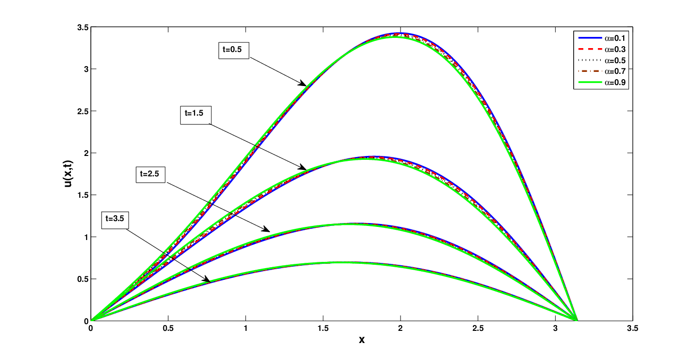
Figure 2: The numerical approximation by the presented method for example 1, with different values of α=0.1,0.3,0.5,0.7,0.9\alpha=0.1,0.3,0.5,0.7,0.9, when β=1.8\beta=1.8 and T=0.5,1.5,2.5,3.5T=0.5,1.5,2.5,3.5.
Refer to caption
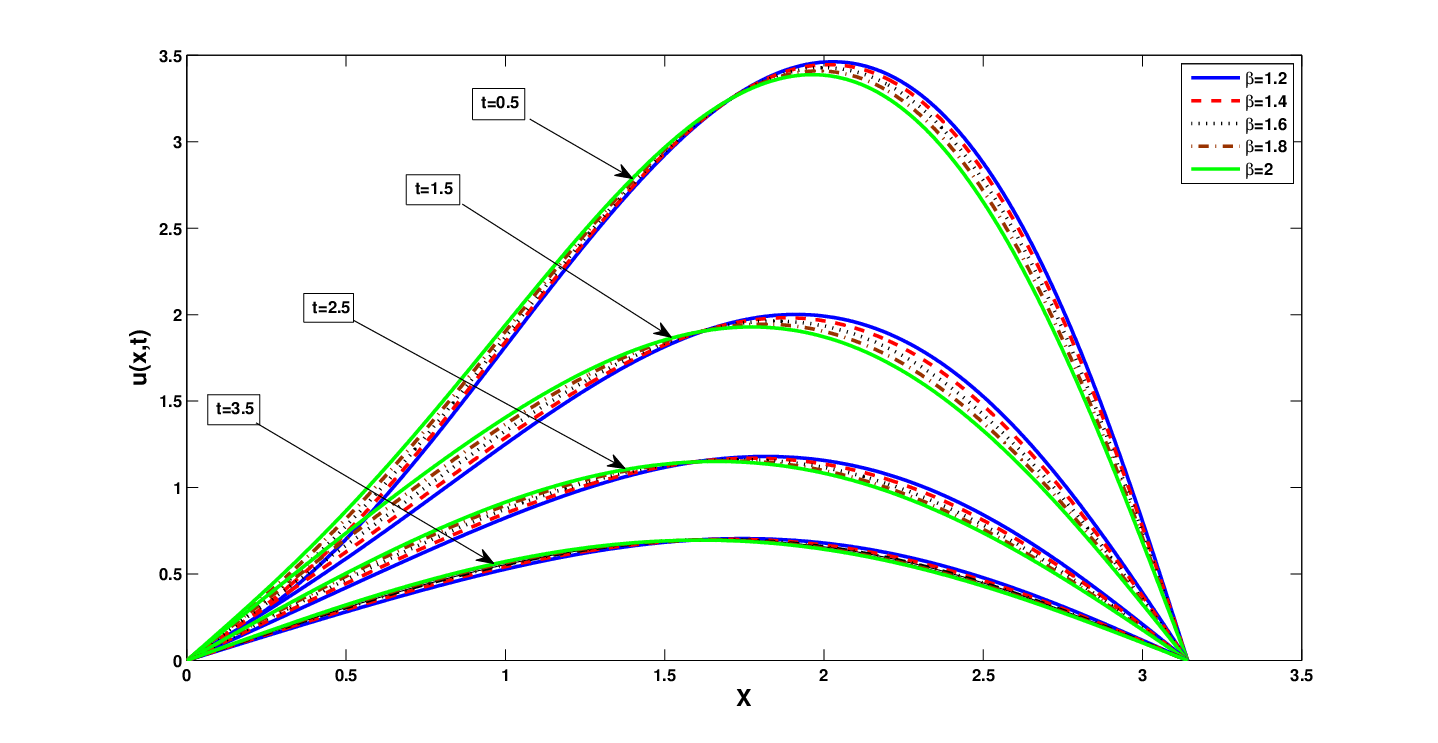
Figure 3: The numerical approximation by the presented method for example 1, with different values of β=1.2,1.4,1.6,1.8,2\beta=1.2,1.4,1.6,1.8,2, when α=0.4\alpha=0.4 and T=0.5,1.5,2.5,3.5T=0.5,1.5,2.5,3.5.
Refer to caption
Figure 4: The numerical approximation and exact solution by the presented method for example3, for α=0.8\alpha=0.8, γ=0.7\gamma=0.7, β=1.2\beta=1.2, when T = 1.
Refer to caption
Figure 5: The numerical approximation by the presented method for example3, for various α=0.1,0.7,0.9,0.95,0.99\alpha=0.1,0.7,0.9,0.95,0.99, when T = 1 and γ=0.3\gamma=0.3, β=1.2\beta=1.2.
Refer to caption
Figure 6: The numerical approximation by the presented method for example3, for various β=1.1,1.6,1.9,2\beta=1.1,1.6,1.9,2, when T = 1 and γ=0.7\gamma=0.7, α=0.9\alpha=0.9.
Refer to caption
Figure 7: The numerical approximation by the presented method for example3, for various γ=0.1,0.3,0.5,0.7,0.9\gamma=0.1,0.3,0.5,0.7,0.9, when T = 1 and α=0.8\alpha=0.8, β=1.2\beta=1.2.

From Table 1 and Figs 2-3, it can be observed that the errors of the presented method are significantly compared with the literature.

Table 1: The absolute errors of the present scheme and numerical method in Yang et al.[26] with α=0.4,β=1.8,t=0.4\alpha=0.4,\,\,\beta=1.8,\,\,\,t=0.4 for 79.
hh Proposed Method order MTM [26] order
π10\frac{\pi}{{10}} 1.55006e-003 - 1.9963e-002 -
π20\frac{\pi}{{20}} 3.9148e-004 1.9796 5.1683e-003 1.9496
π40\frac{\pi}{{40}} 9.8526e-005 1.9898 1.3386e-003 1.9490
π80\frac{\pi}{{80}} 2.4633e-005 1.9999 3.3519e-004 1.9977

Example 2. [26] We consider the following Riesz space fractional advection-dispersion equation with a source term:

∂u⁡(x,t)∂t=Kα∂αu⁡(x,t)∂|x|α+Kβ∂βu⁡(x,t)∂|x|β+f(x,t),    0<t≤T,   0<x<1,u⁡(x,0)=0,u⁡(0,t)=u⁡(1,t)=0,\begin{array}[]{l}\dfrac{{\partial u(x,t)}}{{\partial t}}={K_{\alpha}}\dfrac{{{\partial^{\alpha}}u(x,t)}}{{\partial{{\left|x\right|}^{\alpha}}}}+{K_{\beta}}\dfrac{{{\partial^{\beta}}u(x,t)}}{{\partial{{\left|x\right|}^{\beta}}}}+f(x,t),\,\,\,\,0<t\leq T,\,\,\,0<x<1,\\ u(x,0)=0,\\ u(0,t)=u(1,t)=0,\end{array} (81)

where

f⁡(x,t)=tα−1​eβ​t​(α+β​t)​x2​(1−x)2+Kα​tα​eβ​t2​cos⁡(α​π2)​[24​((1−x)4−α+x4−α)Γ⁡(5−α)−12​((1−x)3−α+x3−α)Γ⁡(4−α)+2​((1−x)2−α+x2−α)Γ⁡(3−α)]+Kβ​tα​eβ​t2​cos⁡(β​π2)[24​((1−x)4−β+x4−β)Γ⁡(5−β)−12​((1−x)3−β+x3−β)Γ⁡(4−β)+2​((1−x)2−β+x2−β)Γ⁡(3−β).]\begin{array}[]{l}f(x,t)={t^{\alpha-1}}{e^{\beta t}}(\alpha+\beta t){x^{2}}{(1-x)^{2}}\\ \,\,\,\,\,\,\,\,\,\,\,\,\,\,\,+\dfrac{{{K_{\alpha}}{t^{\alpha}}{e^{\beta t}}}}{{2\cos(\dfrac{{\alpha\pi}}{2})}}\left[{\dfrac{{24({{(1-x)}^{4-\alpha}}+{x^{4-\alpha}})}}{{\Gamma(5-\alpha)}}-\dfrac{{12({{(1-x)}^{3-\alpha}}+{x^{3-\alpha}})}}{{\Gamma(4-\alpha)}}+\dfrac{{2({{(1-x)}^{2-\alpha}}+{x^{2-\alpha}})}}{{\Gamma(3-\alpha)}}}\right]\\ \,\,\,\,\,\,\,\,\,\,\,\,\,\,\,+\dfrac{{{K_{\beta}}{t^{\alpha}}{e^{\beta t}}}}{{2\cos(\dfrac{{\beta\pi}}{2})}}\left[{\dfrac{{24({{(1-x)}^{4-\beta}}+{x^{4-\beta}})}}{{\Gamma(5-\beta)}}-\dfrac{{12({{(1-x)}^{3-\beta}}+{x^{3-\beta}})}}{{\Gamma(4-\beta)}}+\dfrac{{2({{(1-x)}^{2-\beta}}+{x^{2-\beta}})}}{{\Gamma(3-\beta)}}}.\right]\end{array}

The exact solution of Eq.(81) is given by u⁡(x,t)=tα​eβ​t​x2​(1−x)2.u(x,t)={t^{\alpha}}{e^{\beta t}}{x^{2}}{(1-x)^{2}}.

Table 2: The absolute errors of the present scheme and numerical methods in Yang et al.[26] with α=0.4,β=1.7,t=2\alpha=0.4,\,\,\beta=1.7,\,\,\,t=2 for 81.
hh Proposed Method L1/L2[26] Standard/shifted Grünwald[26]
150\frac{1}{{50}} 5.9364e-004 1.8144e-002 2.8191e-003
1100\frac{1}{{100}} 1.5243e-004 9.4917e-003 1.5093e-003
1200\frac{1}{{200}} 3.8468e-005 4.8584e-003 7.7821e-004
1400\frac{1}{{400}} 9.6028e-006 2.4586e-003 3.9459e-004

The absolute errors of L​1/L​2L1/L2 approximation method and the standard/shifted Grünwald approximation method given in Yang et al.[26] and presented scheme are shown in Tables 2 and they are compared for different values of hh and α=0.4,β=1.7,t=2\alpha=0.4,\,\,\beta=1.7,\,\,\,t=2 and Kα=Kβ=2{K_{\alpha}}={K_{\beta}}=2.
Example 3. We consider the following Riesz space fractional advection-dispersion equation with a source term and delay

∂u⁡(x,t)∂t+∂γu⁡(x,t−1)∂tγ=∂αu⁡(x,t)∂|x|α+∂βu⁡(x,t)∂|x|β+f⁡(x,t),\dfrac{{\partial u(x,t)}}{{\partial t}}+\dfrac{{{\partial^{\gamma}}u(x,t-1)}}{{\partial{{t}^{\gamma}}}}=\dfrac{{{\partial^{\alpha}}u(x,t)}}{{\partial{{\left|x\right|}^{\alpha}}}}+\dfrac{{{\partial^{\beta}}u(x,t)}}{{\partial{{\left|x\right|}^{\beta}}}}+f(x,t), (82)

subject to the initial condition:

u(x,t)=x2(1−x)2t2,−1≤t≤0,   0≤x≤1,u(0,t)=0,u(1,t)=0,  0≤t≤1,\begin{array}[]{l}u(x,t)={x^{2}}{(1-x)^{2}}{t^{2}},\,\,\,-1\leq t\leq 0,\,\,\,0\leq x\leq 1,\\ u(0,t)=0,\,\,u(1,t)=0,\,\,0\leq t\leq 1,\end{array} (83)

where 0<γ<1,  0<α<1,  1<β≤20<\gamma<1,\,\,0<\alpha<1,\,\,1<\beta\leq 2 and

f⁡(x,t)=2​x2​(1−x)2​t+[Γ⁡(3)Γ⁡(3−γ)​t2−γ−2​Γ⁡(2)Γ⁡(2−γ)​t1−γ+Γ⁡(1)Γ⁡(1−γ)​t−γ]​x2​(1−x)2+t22​cos⁡(α​π2)​[24​((1−x)4−α+x4−α)Γ⁡(5−α)−12​((1−x)3−α+x3−α)Γ⁡(4−α)+2​((1−x)2−α+x2−α)Γ⁡(3−α)]+t22​cos⁡(β​π2)​[24​((1−x)4−β+x4−β)Γ⁡(5−β)−12​((1−x)3−β+x3−β)Γ⁡(4−β)+2​((1−x)2−β+x2−β)Γ⁡(3−β)].\begin{array}[]{l}f(x,t)=2{x^{2}}{(1-x)^{2}}t+\left[{\dfrac{{\Gamma(3)}}{{\Gamma(3-\gamma)}}{t^{2-\gamma}}-2\dfrac{{\Gamma(2)}}{{\Gamma(2-\gamma)}}{t^{1-\gamma}}+\dfrac{{\Gamma(1)}}{{\Gamma(1-\gamma)}}{t^{-\gamma}}}\right]{x^{2}}{(1-x)^{2}}\\ \,\,\,\,\,\,\,\,\,\,\,\,\,\,\,+\dfrac{{{t^{2}}}}{{2\cos(\dfrac{{\alpha\pi}}{2})}}\left[{\dfrac{{24({{(1-x)}^{4-\alpha}}+{x^{4-\alpha}})}}{{\Gamma(5-\alpha)}}-\dfrac{{12({{(1-x)}^{3-\alpha}}+{x^{3-\alpha}})}}{{\Gamma(4-\alpha)}}+\dfrac{{2({{(1-x)}^{2-\alpha}}+{x^{2-\alpha}})}}{{\Gamma(3-\alpha)}}}\right]\\ \,\,\,\,\,\,\,\,\,\,\,\,\,\,\,+\dfrac{{{t^{2}}}}{{2\cos(\dfrac{{\beta\pi}}{2})}}\left[{\dfrac{{24({{(1-x)}^{4-\beta}}+{x^{4-\beta}})}}{{\Gamma(5-\beta)}}-\dfrac{{12({{(1-x)}^{3-\beta}}+{x^{3-\beta}})}}{{\Gamma(4-\beta)}}+\dfrac{{2({{(1-x)}^{2-\beta}}+{x^{2-\beta}})}}{{\Gamma(3-\beta)}}}\right].\end{array}

Its exact solution is u⁡(x,t)=x2​(1−x)2​t2u(x,t)={x^{2}}{(1-x)^{2}}{t^{2}}. Some numerical results are reported at Tables 3–5.

Table 3: The absolute errors and the convergence orders of presented method (71) for example 2 with γ=0.5\gamma=0.5.
β=1.2\beta=1.2 β=1.6\beta=1.6 β=1.9\beta=1.9
E​r​r​o​rError O​r​d​e​rOrder E​r​r​o​rError O​r​d​e​rOrder E​r​r​o​rError O​r​d​e​rOrder
α=0.2\alpha=0.2, h=κh=\kappa
1/16 3.8676e-004 – 5.3220e-004 – 6.0947e-004 –
1/32 1.4692e-004 1.40 1.3873e-004 1.94 1.6150e-004 1.92
1/64 4.4836e-005 1.71 3.4679e-005 2.00 4.1138e-005 1.97
1/128 1.2423e-005 1.85 8.5082e-006 2.02 1.0283e-005 2.00
α=0.5\alpha=0.5, h=κh=\kappa
1/16 2.4977e-004 – 4.2841e-004 – 5.3059e-004 –
1/32 1.1031e-004 1.18 1.1294e-004 1.92 1.4195e-004 1.90
1/64 3.6830e-005 1.58 2.8289e-005 2.00 3.6317e-005 1.97
1/128 1.0832e-005 1.77 7.1049e-006 2.00 9.0898e-006 2.00
Table 4: The absolute errors and the convergence orders of presented method (71) for example 2 with β=1.9\beta=1.9.
α=0.2\alpha=0.2 α=0.5\alpha=0.5 α=0.8\alpha=0.8
E​r​r​o​rError O​r​d​e​rOrder E​r​r​o​rError O​r​d​e​rOrder E​r​r​o​rError O​r​d​e​rOrder
γ=0.2\gamma=0.2, h=κh=\kappa
1/16 6.0947e-004 – 5.3059e-004 – 2.9416e-004 –
1/32 1.6150e-004 1.92 1.4195e-004 1.90 9.3235e-005 1.67
1/64 4.1138e-005 1.97 3.6317e-005 1.97 2.5705e-005 1.86
1/128 1.0283e-005 2.00 9.0898e-006 2.00 6.6475e-006 1.95
Table 5: The absolute errors and the convergence orders of presented method (71) for example 2 with α=0.1\alpha=0.1.
β=1.2\beta=1.2 β=1.6\beta=1.6 β=1.9\beta=1.9
E​r​r​o​rError O​r​d​e​rOrder E​r​r​o​rError O​r​d​e​rOrder E​r​r​o​rError O​r​d​e​rOrder
γ=0.7\gamma=0.7, h=κh=\kappa
1/16 4.0456e-004 – 5.5129e-004 – 6.2364e-004 –
1/32 1.5142e-004 1.42 1.4380e-004 1.94 1.6524e-004 1.92
1/64 4.5762e-005 1.73 3.5984e-005 2.00 4.2094e-005 1.97
1/128 1.2597e-005 1.86 8.8387e-006 2.02 1.0524e-005 2.00

8 Conclusion

In this paper, the fractional backward differential formulas method and shifted Grünwald difference (WSGD) operators are used to approximate the Riesz space fractional derivative. The presented numerical method is proposed and applied to solve the Riesz space fractional advection-dispersion equations with delay. We prove that the difference scheme is conditionally stable and convergent with the accuracy O⁡(κ2+h2){\rm O}({\kappa^{2}}+{h^{2}}). Furthermore, the analytical solution for RFADED in terms of the functions of Mittag–Leffler type has been obtained. Finally, some results are given to demonstrate the effectiveness of theoretical analysis. In the future, we would like to investigate this method and technique of high order for solving this problem.

References

References

  • [1] R. L. Bagley, R. Calico, Fractional order state equations for the control of viscoelasticallydamped structures, Journal of Guidance, Control, and Dynamics 14 (2) (1991) 304–311.
  • [2] W. Weaver Jr, S. P. Timoshenko, D. H. Young, Vibration problems in engineering, John Wiley & Sons, 1990.
  • [3] R. J. Marks, M. W. Hall, et al., Differintegral interpolation from a bandlimited signal’s samples, Acoustics, Speech and Signal Processing, IEEE Transactions on 29 (4) (1981) 872–877.
  • [4] H. Simo, P. Woafo, Effects of asymmetric potentials on bursting oscillations in duffing oscillator, Optik-International Journal for Light and Electron Optics 127 (20) (2016) 8760–8766.
  • [5] I. Podlubny, Fractional differential equations: An introduction to fractional derivatives, fractional differential equations, to methods of their solution and some of their applications, vol. 198 of, Mathematics in Science and Engineering.
  • [6] A. A. A. Kilbas, H. M. Srivastava, J. J. Trujillo, Theory and applications of fractional differential equations, Vol. 204, Elsevier Science Limited, 2006.
  • [7] J. Wu, Theory and applications of partial functional differential equations, Vol. 119, Springer Science & Business Media, 2012.
  • [8] L. Galeone, R. Garrappa, On multistep methods for differential equations of fractional order, Mediterranean Journal of Mathematics 3 (3-4) (2006) 565–580.
  • [9] R. Garrappa, Trapezoidal methods for fractional differential equations: Theoretical and computational aspects, Mathematics and Computers in Simulation 110 (2015) 96–112.
  • [10] R. Gorenflo, Fractional calculus: Some numerical methods, fractals and fractional calculus in continuum mechanics, CISM Lecture Notes, Springer Verlag, Wien (1997) 277–290.
  • [11] C. Lubich, Discretized fractional calculus, SIAM Journal on Mathematical Analysis 17 (3) (1986) 704–719.
  • [12] M. S. Heris, M. Javidi, A predictor–corrector scheme for the tempered fractional differential equations with uniform and non-uniform meshes, The Journal of Supercomputing 75 (12) (2019) 8168–8206.
  • [13] M. Javidi, M. S. Heris, B. Ahmad, A predictor-corrector scheme for solving nonlinear fractional differential equations with uniform and nonuniform meshes., Int. J. Model. Simul. Sci. Comput. 10 (5) (2019) 1950033–1.
  • [14] Z. Wang, X. Huang, G. Shi, Analysis of nonlinear dynamics and chaos in a fractional order financial system with time delay, Computers & Mathematics with Applications 62 (3) (2011) 1531–1539.
  • [15] M. S. Heris, M. Javidi, On fractional backward differential formulas for fractional delay differential equations with periodic and anti-periodic conditions, Applied Numerical Mathematics 118 (2017) 203–220.
  • [16] M. S. Heris, M. Javidi, On fbdf5 method for delay differential equations of fractional order with periodic and anti-periodic conditions, Mediterranean Journal of Mathematics 14 (3) (2017) 134.
  • [17] M. L. Morgado, N. J. Ford, P. M. Lima, Analysis and numerical methods for fractional differential equations with delay, Journal of computational and applied mathematics 252 (2013) 159–168.
  • [18] J. Čermák, J. Horníček, T. Kisela, Stability regions for fractional differential systems with a time delay, Communications in Nonlinear Science and Numerical Simulation 31 (1-3) (2016) 108–123.
  • [19] Z. Wang, X. Huang, J. Zhou, A numerical method for delayed fractional-order differential equations: based on gl definition, Appl. Math. Inf. Sci 7 (2) (2013) 525–529.
  • [20] B. Zubik-Kowal, Chebyshev pseudospectral method and waveform relaxation for differential and differential–functional parabolic equations, Applied numerical mathematics 34 (2-3) (2000) 309–328.
  • [21] Z. Jackiewicz, B. Zubik-Kowal, Spectral collocation and waveform relaxation methods for nonlinear delay partial differential equations, Applied Numerical Mathematics 56 (3-4) (2006) 433–443.
  • [22] J. Tanthanuch, Symmetry analysis of the nonhomogeneous inviscid burgers equation with delay, Communications in Nonlinear Science and Numerical Simulation 17 (12) (2012) 4978–4987.
  • [23] C. Tadjeran, M. M. Meerschaert, H.-P. Scheffler, A second-order accurate numerical approximation for the fractional diffusion equation, Journal of Computational Physics 213 (1) (2006) 205–213.
  • [24] Q. Liu, F. Zeng, C. Li, Finite difference method for time-space-fractional schrödinger equation, International Journal of Computer Mathematics 92 (7) (2015) 1439–1451.
  • [25] H. Ding, C. Li, Numerical algorithms for the fractional diffusion-wave equation with reaction term, in: Abstract and Applied Analysis, Vol. 2013, Hindawi Publishing Corporation, 2013.
  • [26] Q. Yang, F. Liu, I. Turner, Numerical methods for fractional partial differential equations with riesz space fractional derivatives, Applied Mathematical Modelling 34 (1) (2010) 200–218.
  • [27] S. Momani, Z. Odibat, Numerical solutions of the space-time fractional advection-dispersion equation, Numerical Methods for Partial Differential Equations 24 (6) (2008) 1416–1429.
  • [28] F. Liu, V. V. Anh, I. Turner, P. Zhuang, Time fractional advection-dispersion equation, Journal of Applied Mathematics and Computing 13 (1) (2003) 233–245.
  • [29] F. Huang, F. Liu, The fundamental solution of the space-time fractional advection-dispersion equation, Journal of Applied Mathematics and Computing 18 (1) (2005) 339–350.
  • [30] M. M. Meerschaert, H.-P. Scheffler, C. Tadjeran, Finite difference methods for two-dimensional fractional dispersion equation, Journal of Computational Physics 211 (1) (2006) 249–261.
  • [31] H. Zhang, F. Liu, The fundamental solutions of the space, space-time riesz fractional partial differential equations with periodic conditions, NUMERICAL MATHEMATICS-ENGLISH SERIES- 16 (2) (2007) 181.
  • [32] J. Chen, F. Liu, I. Turner, V. Anh, The fundamental and numerical solutions of the riesz space-fractional reaction–dispersion equation, The ANZIAM Journal 50 (1) (2008) 45–57.
  • [33] H. Zhang, F. Liu, V. Anh, Galerkin finite element approximation of symmetric space-fractional partial differential equations, Applied Mathematics and Computation 217 (6) (2010) 2534–2545.
  • [34] S. Shen, F. Liu, V. Anh, I. Turner, J. Chen, A novel numerical approximation for the space fractional advection–dispersion equation, IMA journal of Applied Mathematics 79 (3) (2014) 431–444.
  • [35] C. Çelik, M. Duman, Crank–nicolson method for the fractional diffusion equation with the riesz fractional derivative, Journal of computational physics 231 (4) (2012) 1743–1750.
  • [36] H. Ding, C. Li, Y. Chen, High-order algorithms for riesz derivative and their applications (i), Abstr. Appl. Anal 653797.
  • [37] H. Ding, C. Li, Y. Chen, High-order algorithms for riesz derivative and their applications (ii), Journal of Computational Physics 293 (2015) 218–237.
  • [38] H. Ding, C. Li, High-order algorithms for riesz derivative and their applications (iii), Fractional Calculus and Applied Analysis 19 (1) (2016) 19–55.
  • [39] H. Ding, C. Li, High-order algorithms for riesz derivative and their applications (v), Numerical Methods for Partial Differential Equations 33 (5) (2017) 1754–1794.
  • [40] M. M. Meerschaert, C. Tadjeran, Finite difference approximations for fractional advection–dispersion flow equations, Journal of Computational and Applied Mathematics 172 (1) (2004) 65–77.
  • [41] F. Liu, V. Anh, I. Turner, Numerical solution of the space fractional fokker–planck equation, Journal of Computational and Applied Mathematics 166 (1) (2004) 209–219.
  • [42] S. Shen, F. Liu, V. Anh, Fundamental solution and discrete random walk model for a time-space fractional diffusion equation of distributed order, Journal of Applied Mathematics and Computing 28 (1) (2008) 147–164.
  • [43] S. Shen, F. Liu, V. Anh, Numerical approximations and solution techniques for the space-time riesz–caputo fractional advection-diffusion equation, Numerical Algorithms 56 (3) (2011) 383–403.
  • [44] E. Sousa, A second order explicit finite difference method for the fractional advection diffusion equation, Computers & Mathematics with Applications 64 (10) (2012) 3141–3152.
  • [45] M. Ilic, F. Liu, I. Turner, V. Anh, Numerical approximation of a fractional-in-space diffusion equation, i, Fractional Calculus and Applied Analysis 8 (3) (2005) 323–341.
  • [46] P. Henrici, Discrete variable methods in ordinary differential equations, New York: Wiley, 1962 1.
  • [47] P. Wolkenfelt, Linear multistep methods and the construction of quadrature formulae for volterra integral and integro-differential equations, Stichting Mathematisch Centrum. Numerieke Wiskunde (76/79) (1979) 1–47.
  • [48] D. Zeilberger, The jcp miller recurrence for exponentiating a polynomial, and its q-analog*, Journal of Difference Equations and Applications 1 (1) (1995) 57–60.
  • [49] R. Garrappa, Trapezoidal methods for fractional differential equations: Theoretical and computational aspects, Mathematics and Computers in Simulation 110 (2015) 96–112.
  • [50] W. Tian, H. Zhou, W. Deng, A class of second order difference approximations for solving space fractional diffusion equations, Mathematics of Computation 84 (294) (2015) 1703–1727.
  • [51] J. W. Thomas, Numerical partial differential equations: finite difference methods, Vol. 22, Springer Science & Business Media, 2013.
  • [52] R. S. Varga, Geršgorin and his circles, Vol. 36, Springer Science & Business Media, 2010.