Asymptotic Task-Based Quantization with Application to Massive MIMO Parts of this work were presented in the 2019 IEEE International Conference on Acoustics, Speech, and Signal Processing (ICASSP), Brighton, UK.This project has received funding from the European Union’s Horizon 2020 research and innovation program under grant No. 646804-ERC-COG-BNYQ, from the Israel Science Foundation under grant No. 0100101, and from the Royal Society International Exchange scheme IE 160348. N. Shlezinger and Y. C. Eldar are with the faculty of Math and CS, Weizmann Institute of Science, Rehovot, Israel (e-mail: nirshlezinger1@gmail.com; yonina@weizmann.ac.il). M. R. D. Rodrigues is with the department of EE, University College, London, UK (e-mail: m.rodrigues@ucl.ac.uk).
Abstract
Quantizers take part in nearly every digital signal processing system which operates on physical signals. They are commonly designed to accurately represent the underlying signal, regardless of the specific task to be performed on the quantized data. In systems working with high-dimensional signals, such as massive multiple-input multiple-output (MIMO) systems, it is beneficial to utilize low-resolution quantizers, due to cost, power, and memory constraints. In this work we study quantization of high-dimensional inputs, aiming at improving performance under resolution constraints by accounting for the system task in the quantizers design. We focus on the task of recovering a desired signal statistically related to the high-dimensional input, and analyze two quantization approaches: We first consider vector quantization, which is typically computationally infeasible, and characterize the optimal performance achievable with this approach. Next, we focus on practical systems which utilize hardware-limited scalar uniform analog-to-digital converters (ADCs), and design a task-based quantizer under this model. The resulting system accounts for the task by linearly combining the observed signal into a lower dimension prior to quantization. We then apply our proposed technique to channel estimation in massive MIMO networks. Our results demonstrate that a system utilizing low-resolution scalar ADCs can approach the optimal channel estimation performance by properly accounting for the task in the system design.
I Introduction
Digital signal processing and communications systems use quantized representations of continuous-amplitude physical quantities [1]. These digital representations are typically designed to accurately match the original analog signal, by minimizing some distortion measure between the analog signal and the digital representation [2], regardless of the task of the system. Nonetheless, in many cases, the system task is not to recover the analog signal, but to extract some other information from its quantized representation [3]. It is therefore possible that in such systems – which we refer to as task-based quantizers – one can obtain further performance improvements in terms of the quantization rate necessary to achieve a certain performance.
Practical quantizers typically utilize scalar uniform adc [1]. Recent years have witnessed a growing interest in systems operating with quantized large-scale vectors obtained using low-resolution scalar adc. One of the main applications considered is massive mimo (mimo) communications [4, 5, 6, 13, 11, 12, 15, 7, 14, 8, 17, 10, 9, 16, 18], which is a key technology for the realization of next generation wireless networks [19]. In such systems, a wireless bs (bs) is equipped with a large number of antennas [20, 21, 22]. The bs first quantizes the received signal using a set of adc, commonly implementing scalar uniform quantization. Then, the quantized representation is used to estimate the underlying channel [4, 5, 6, 7, 8, 9, 10] and/or recover the transmitted messages [11, 13, 12, 5, 6, 15, 14, 7, 8, 9, 10, 16, 17]. For large-scale inputs, i.e., large number of bs antennas, accurate quantizers become costly in terms of power and memory usage, particularly when utilizing a large bandwidth, making low-resolution quantization essential for realizing massive mimo systems [19]. As the task in massive mimo is not to recover the input signal, but to estimate the channel or decode the transmitted message, reasonable performance with low-resolution scalar quantizers has been observed [4, 5, 6, 13, 11, 12, 15, 7, 14, 8, 9, 10, 16, 17, 18]. However, most prior works assume that the quantizers are fixed, commonly assuming one-bit sign quantization [16, 9, 6, 5]. Thus, they do not characterize the achievable performance when the quantizers are designed to account for the system task.
In the presence of multivariate inputs, joint (vector) quantization is known to outperform scalar quantization [23, Ch. 10]. Task-based vector quantization can be considered as an indirect lossy-source coding setup [2]. In such scenarios, one wishes to recover a desired source based on a discrete representation of its noisy version, in the sense of minimizing a given distortion measure [24]. For the mse distortion, it was shown in [25] that the optimal system which achieves the rate-distortion curve, namely, uses the minimal number of bits per input sample required to achieve a fixed distortion, applies vector quantization to the mmse (mmse) estimate of the desired source. This observation was used in [26, 27] to study sampling and vector quantization of continuous-time signals. Nonetheless, in the presence of high-dimensional inputs, vector quantization becomes infeasible, so that practical task-based quantization approaches are required.
Task-based quantization with scalar uniform adc, referred to as hardware-limited task-based quantization, can be realized by allowing analog linear processing prior to quantization [28]. mimo communications systems utilizing both analog and digital processing are known as hybrid architectures [12, 29, 30], and are the focus of a large amount of recent works. In particular, [31] compared the achievable-rate versus power efficiency tradeoff for various analog combining systems, [12] and [32] designed hybrid architectures aimed at maximizing the achievable rate and signal recovery mse, respectively, with full csi (csi), while [13] studied bit allocation for minimizing the quantization error when the analog combining is set to the largest channel eigenmodes, using high rate quantization analysis. Additionally, [14] studied the achievable rate with imperfect csi when distinct sets of inputs are each combined in the analog domain to maximize the receive power, while [33] characterized bounds on the capacity of mimo communications with analog combining and one-bit quantizers. Most previous works which designed hybrid mimo receivers, e.g., [12, 13, 32], considered finite-size inputs and required csi in their design, and thus cannot be utilized for massive mimo channel estimation. Specifically, the joint design of analog combining, quantization rule, and digital processing, to optimize the accuracy of massive mimo channel estimation with scalar adc has not yet been studied, to the best of our knowledge.
In this work we study task-based quantization for channel estimation in massive mimo systems operating with scalar adc. Our analysis is based on an extension of the hardware-limited task-based quantization framework proposed in our previous work [28], which studied parameter estimation from a finite-sized quantized observed signal. The work [28] proposed to jointly optimize the analog combining, quantization rule, and digital processing, to minimize the mse in recovering the desired finite-sized vector. Here, we extend the study of [28] to account for asymptotically large data, developing a framework for task-based quantization with high-dimensional inputs, and then apply the resulting analysis to massive mimo systems, which are commonly studied in the asymptotic number of antennas regime [20, 21]. In particular, we focus on massive mimo channel estimation, carried out in a tdd (tdd) manner [20, 21, 22]. Unlike previous works on hybrid architectures optimization with low-resolution quantization, e.g., [12, 13, 32], our work does not require knowledge of the channel. In fact, in the presence of adjustable analog combining hardware, such as dynamic metasurface antennas [34], our analysis can be combined with previously proposed hybrid systems by reconfiguring the analog combining hardware once the channel is accurately estimated. We also note that our analysis can be applied to different tasks, such as signal recovery and noise mitigation.
We begin by studying task-based vector quantization using indirect lossy source coding theory. We characterize the minimal achievable average mse for any quantization system operating with a fixed quantization rate, namely, a fixed number of bits per input sample. Then, we study the performance when vector quantization is carried out independently from the task, referred to as task-ignorant vector quantization. Since the input dimensionality here is asymptotically large, we are able to explicitly obtain the achievable performance, unlike [28], using indirect rate-distortion theory. Studying vector quantizers allows us to quantify the performance bounds of task-based quantization with large-scale inputs, and in particular, understand the fundamental limits of massive mimo channel estimation.
Next, we study task-based quantization with scalar uniform adc, allowing analog combining prior to quantization. While analog combining can contribute in aspects other than improving the performance with finite-resolution quantizers, e.g., reducing the number of costly RF chains in massive mimo systems [32], we focus here on the achievable performance for a given quantization rate. For this setup we propose a task-based quantization system with linear analog and digital processing which minimizes the average mse under such hardware-limited structure constraints. We show that, unlike in the fixed size regime studied in [28], for large-scale inputs an important parameter which greatly affects the system performance is the analog combining ratio, which determines how the number of scalar quantizers grows as the input size tends to infinity.
Then, we focus on massive mimo systems, and show how the proposed task-based quantization system can be applied to channel estimation from quantized measurements. We note that in this scenario the inputs are gathered over different antennas as well as over different time instances. Since in some cases, it may be desirable to combine only samples received at the same time instance, to avoid introducing delays in the analog domain, we also derive the system which minimizes the average mse subject to the constraint that only inputs taken at the same time instance can be combined. This constraint reduces the complexity of the resulting system at the cost of degraded mse performance. In our numerical study, we illustrate the fundamental performance limits of massive mimo channel estimation achievable using vector quantizers, and compare these limits to our proposed task-based quantization systems with scalar adc, and to massive mimo channel estimators which operate only in the digital domain. Our results demonstrate that the proposed quantizers, which utilize practical low-resolution scalar adc, are capable of approaching the optimal performance, achievable using vector quantizers, and outperform previously proposed estimators.
The rest of this paper is organized as follows: Section II reviews some basics in quantization theory. Section III extends the results of [28] to large-scale data, and Section IV applies them to massive mimo channel estimation. Section V provides simulation examples. Finally, Section VI concludes the paper.
Throughout the paper, we use boldface lower-case letters for vectors, e.g., ; the th element of is written as . Matrices are denoted with boldface upper-case letters, e.g., , and we use to denote its th element. We use to denote the identity matrix. Sets are expressed with calligraphic letters, e.g., , and is the th order Cartesian power of . Hermitian transpose, transpose, complex conjugate, stochastic expectation, and mutual information are written as , , , , and , respectively. For a real number , we use ; denotes the integer divisor (plus one) of the value in the brackets (minus one), namely, . We use to denote the trace operator, is the indicator function, is the Kronecker product, and are the sets of real and complex numbers, respectively. All logarithms are taken to base-2. Finally, for an matrix , is the vector obtained by stacking the columns of .
II Preliminaries in Quantization Theory
To formulate the task-based quantization setup. we first briefly review standard quantization notions. While parts of this review also appear in our previous work [28], it is included for completeness. We begin with the definition of a quantizer:
Definition 1 (Quantizer).
A quantizer with bits, input size , input alphabet , output size , and output alphabet , consists of: 1) An encoding function which maps the input from into a discrete index . 2) A decoding function which maps each index into a codeword .
The quantizer output for input is . Scalar quantizers operate on a scalar input, i.e., and is a scalar space, while vector quantizers have a multivariate input. Note that when is a vector space, then each is a random vector. When the input size and output size are equal, namely, , we write .
In the standard quantization problem, a quantizer is designed to minimize some distortion measure between its input and its output. The performance of a quantizer is therefore characterized using two measures: The quantization rate, defined as , and the expected distortion . For a fixed input size and codebook size , the optimal quantizer is given by
| (1) |
Characterizing the optimal quantizer via (1) and the optimal tradeoff between distortion and quantization rate is in general a very difficult task. Consequently, optimal quantizers are typically studied assuming either high quantization rate, i.e., , see, e.g., [35], or asymptotically large input size, namely, , typically with stationary inputs, via rate-distortion theory [23, Ch. 10]. For example, when the quantizer input represents a stationary source, and the distortion measure is subadditive, i.e., for any , , , , , , it holds that . Then, by [36, Thm. 5.9.1] the optimal distortion in the limit for a fixed rate is given by the distortion-rate function:
Definition 2 (Distortion-rate function).
The distortion-rate function for a stationary source with respect to the subadditive distortion measure is defined as
| (2) |
The minimization in (2) is carried out over all conditional distributions which satisfy the given constraint on the resulting mutual information. The marginal output distribution of which obtains the minima in (2) is referred to henceforth as the optimal marginal distortion-rate distribution. One scenario where is given in closed-form is when each is a zero-mean proper-complex Gaussian rv (rv) [37, Def. 1], i.e., , such that for each , the source is stationary11 1 Following [36], we use the term stationary source for stationary and ergodic signals with time index . with scalar psd (psd) , thus its multivariate psd is . The distortion-rate function for this scenario is given in the following example:
Example 1.
Let be zero-mean proper-complex Gaussian source with multivariate psd , and let the eigenvalue decomposition of be given by . The distortion-rate function for with the mse distortion is [38, Cor. 1]
| (3a) | |||
| where is the solution to | |||
| (3b) | |||
| The optimal marginal distribution for this setup is a zero-mean proper-complex multivariate Gaussian distribution with psd , where is a diagonal matrix with diagonal entries . | |||
Comparing high rate analysis for scalar quantizers and rate-distortion theory for vector quantizers demonstrates the sub-optimality of serial scalar quantization. For example, for quantizing a large-scale real-valued Gaussian random vector with i.i.d. entries and sufficiently large quantization rate , where one would imagine there is little benefit in quantizing the entries jointly over quantizing each entry independently, vector quantization notably outperforms serial scalar quantization [39, Ch. 23.2].
Finally, we introduce the notion of dithered quantization, which will be frequently used in our analysis of hardware-limited task-based quantization systems:
Definition 3 (Dithered quantizer).
A scalar quantizer implements serial non-subtractive uniform dithered quantization [40], referred to henceforth as dithered quantization, with support and quantization spacing , if its output for an input sequence can be written as . Here, are i.i.d. rv with i.i.d. real and imaginary parts uniformly distributed over , mutually independent of the input, and implements uniform quantization defined as
Note that when , the uniform quantizer is a standard one-bit sign quantizer of the form , where the is determined by the support .
In the following we study hardware-limited systems assuming dithered quantizers. Our motivation for using dithered quantizers stems from the fact that conventional analysis of uniform quantizers, e.g., [41], does not lead to a tractable model for the quantizer output, nor does it extend to the task-based setup. However, when using dithered quantizers, the digital representation of an input which is in the support of the quantizer can be written as the sum of the quantizer input and an additive uncorrelated white noise signal [40]. This significantly facilitates our analysis and allows to characterize the system which minimizes the mse. Nonetheless, it is emphasized that this property of dithered quantizers is also approximately satisfied in uniform quantization without dithering for various input distributions, including Gaussian inputs22 2 For a Gaussian input with magnitude smaller than with sufficiently high probability, if the quantization spacing is in the order of the input standard deviation (or smaller), then the output can be modeled as the input corrupted by additive uncorrelated white noise, even without dithering [42, Sec. VII]. [42]. Therefore, the rigorous analysis which follows from considering dithered quantization, also holds approximately when using standard uniform quantizers without dithering, as demonstrated in [28].
III Task-Based Quantization of Large-Scale Data
We now extend the analysis of task-based quantization carried out in our previous work [28], which considered fixed-size signals, to asymptotically large input signals. The motivation of this extension stems from the need to properly design and characterize quantizers for massive mimo systems, which is our main target application discussed in Section IV. To that aim, we first present the problem formulation in Subsection III-A, and derive the achievable mse without quantization constraints in Subsection III-B. Then, we study task-based quantization with vector quantizers in Subsection III-C and with hardware-limited quantizers in Subsection III-D. Focusing on the asymptotic regime allows us to rigorously characterize the achievable performance of vector quantizers, for which we were only able to obtain bounds in the finite horizon case studied in [28]. For the hardware-limited case, we formulate the dependency of task-based quantization systems on how the system parameters grow proportionally with the size of the input signal, i.e., the quantization rate and the analog combining ratio.
III-A Problem Formulation
We study task-based quantization with asymptotically large observations and a proportionally large desired signal. The design objective of the quantizer is to quantize the observations such that the desired signal can be accurately recovered from the quantized observations in the sense of minimizing the mse. The desired signal consists of zero-mean random vectors , sampled from a stationary source with multivariate autocorrelation function , where is Hermitian and positive semi-definite, while is an absolutely summable scalar autocorrelation function satisfying . By letting be the dtft (dtft) of , the corresponding multivariate psd is given by . The observations are a set of random vectors with multivariate psd , where , and each vector is related to its corresponding via the same conditional probability measure, denoted . The model assumption that the size of the desired signal is not larger than that of the observed signal allows us to clearly demonstrate the benefits of task-based quantization as noted in [28], and faithfully represent our main target application of channel estimation in massive mimo systems discussed in Section IV.
We assume that the mmse estimator which stems from is linear, i.e., there exists such that the mmse estimate of from can be written as , for each . Since we focus on large-scale data, is arbitrarily large. Clearly, this setup specializes to the case in which the desired signal and the observed signal consist of i.i.d. elements. Such scenarios arise, for example, in signal recovery over memoryless channels, where is the channel input at time index and is the corresponding channel output, or alternatively, in the estimation of fast fading memoryless channels, in which is the unknown channel at time index and is the channel output. Furthermore, in Section IV we show that this model can also represent channel estimation in massive mimo systems with correlated antennas.
We write the desired vector and the observed vector as and , respectively. By letting be a Toeplitz matrix whose entries are given by for each , it holds that the covariance matrices of and are equal to and , respectively. The main model notations along with their meaning in the massive mimo setup considered in Section IV are summarized in Table I. The proposed system forms a quantized representation of based on the observed , using up to bits, where the quantization rate is fixed. An illustration of such a system is depicted in Fig. 1.

| Notation | Type | General Setup (Section III) | Massive mimo Setup (Section IV) |
|---|---|---|---|
| Large integer | Number of observations | Number of antennas | |
| Integer | Size of desired signal samples | Number of users in cell | |
| Integer | Size of observation samples | Number of pilot symbols | |
| complex vector | Desired signal | Channel coefficients in vector form | |
| complex vector | Observations | Channel outputs in vector form | |
| complex matrix | Linear mmse matrix | Linear mmse matrix | |
| complex matrix | Covariance of each observed sample | Temporal covariance of channel outputs | |
| real numbers | Singular values of | Singular values of | |
| Mapping | Entry-wise correlation | Spatial correlation between antennas | |
| complex matrix | Toeplitz matrix constructed from | Spatial correlation matrix | |
| Mapping | dtft of | Spatial psd of each channel output | |
| Real number | Quantization rate | Quantization rate | |
| Integer | Number of scalar quantizers | Number of scalar quantizers | |
| Real number | Analog combining ratio | Analog combining ratio | |
| Integer | Number of scalar quantization regions | Number of scalar quantization regions | |
| Real number | Scalar quantizer support | Scalar quantizer support |
The distortion measure for a quantized representation is the average mse, defined as
| (4) |
We consider vector quantizers as well as hardware-limited quantizers. In the following we elaborate on these systems:
Vector Quantizers: Joint (vector) quantization is known to be superior to separate (scalar) quantization [39, Ch. 23]. Thus, analyzing systems utilizing vector quantizers provides the fundamental limits of task-based quantization with large-scale inputs. We consider two different vector quantization systems:
- 1.
Task-based optimal vector quantization - in the optimal quantization system, the quantizer in Fig. 1 is the vector quantizer which minimizes the distortion between the quantized representation and . The performance of this system represents the optimal distortion achievable with any quantization system operating at rate .
- 2.
Task-ignorant vector quantization - here, the quantizer is designed to recover the observed separately from the task, using the optimal vector quantizer for representing , namely, the quantizer here is ignorant of the task and is designed to accurately represent the observations. The desired vector is estimated from the quantized representation using the mmse estimator, as illustrated in Fig. 2. This is a plausible system when the quantizer is ignorant of the task.

Hardware-Limited Quantizers: Vector quantization may be difficult to implement, especially for large input sizes. Consequently, systems utilizing vector quantizers may not be feasible in practice. As discussed in the introduction, practical systems typically implement quantization using scalar adc. In such systems, each continuous-amplitude element is converted into a discrete representation using a single quantization rule, which commonly corresponds to uniform quantization. This operation can be modeled using identical scalar uniform quantizers. In particular, we consider the system depicted in Fig. 3.
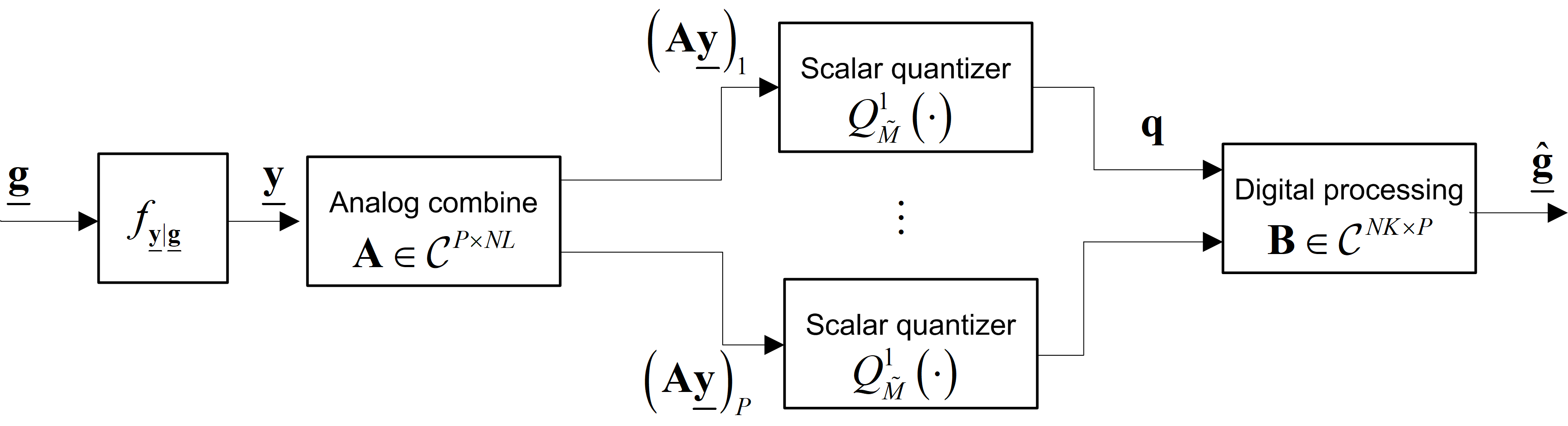
The observed vector , is projected into , where , using some pre-quantization processing carried out in the analog domain. As arbitrary processing may be difficult to implement in analog, we henceforth restrict our attention to linear pre-quantization processing only. This analog combining is modeled via the matrix . We write the number of scalar quantizers in terms of its integer quotient and remainder with respect to , denoted and , respectively, i.e.,
| (5) |
The motivation for expressing using in (5) stems from the fact that for large-scale inputs, tends to infinity, and thus and represent how scales accordingly. These scaling parameters play an important role when analyzing the performance of hardware-limited task-based quantizers, as shown in Subsection III-D.
The real and imaginary parts of each entry of are quantized using the same scalar quantizer with resolution , denoted . Define the analog combining ratio
| (6) |
Note that . The overall quantization rate is . The identical scalar quantizers implement dithered quantization, as defined in Def. 3. The quantizer is designed to operate within the support , namely, the amplitude of the input is not larger than with sufficiently large probability. To guarantee this, we fix to be some multiple of the maximal standard deviation of the input. For example, for proper-complex Gaussian inputs, when the amplitude of both the real and imaginary parts of the input are smaller than the support with probability over . We assume that , such that the variable is strictly positive. Note that satisfies this requirement for any , i.e., the adc is implemented using scalar quantizers with at least one bit.
Finally, in the digital domain, the system approximates the linear mmse estimate based on the output of the adc, denoted , where . Consequently, the estimate can be written as for some . We focus on linear digital processing to keep the analysis tractable, and since linear estimators are commonly used in our main application, massive mimo channel estimation with quantized outputs [5, 7]. This restriction is not expected to notably affect the overall performance, especially when the error due to quantization is small, as the mmse estimator in the considered setup is linear.
III-B No Quantization Constraints
As a preliminary step, we note that the mmse estimate of from , denoted consists of the random vectors , sampled from a stationary source with multivariate psd . Since , the average mmse can be written as
| (7) |
The mmse in (7) is achievable without quantization, and thus serves as a lower bound on the achievable distortion of the quantization systems discussed in the following subsections.
III-C Vector Quantization
We now study the average mse achievable of the vector quantization systems detailed in Subsection III-A. We note that for fixed size inputs, the achievable performance of vector quantizers can only be obtained in terms of upper and lower bounds, see [28, Prop. 1]. However, as we show next, for large-scale data, we explicitly characterize the minimal achievable average mse for each system using indirect rate-distortion theory analysis, which considers asymptotically large inputs.
III-C1 Optimal Vector Quantizer
The optimal vector quantizer minimizes the mse between the unknown desired vector and the system output. Recovering the desired signal from quantized observations is a special case of indirect lossy source coding [24]. For the mse distortion, it follows from [25] that the optimal vector quantizer first recovers the mmse estimate , and then uses a vector quantizer to represent . The resulting mse is given in the following theorem:
Theorem 1.
The mse of the optimal vector quantizer is
| (8) |
where is the distortion-rate function, given in Def. 2, of the random vector with the mse distortion.
Proof: See Appendix -A.
Theorem 1 holds since the mmse estimate represents a stationary source, thus, in the limit , the minimal mse for a fixed quantization rate is given by the distortion-rate function. The achievable average mse in (8) constitutes the minimal achievable distortion of any system which recovers from using up to bits per input sample.
III-C2 Task-Ignorant Vector Quantizer
In task-ignorant quantization, the desired signal is estimated from the quantized observations, which are in turn designed to yield an accurate representation of the input signal. The resulting quantization system, depicted in Fig. 2, first quantizes via a quantizer , which minimizes the mse between its output and . Then, is estimated from the output of the quantizer using the mmse estimator. Characterizing the average mse of such systems is in general a challenging task, due to difficulty in formulating the conditional distribution of the desired signal given the output of the quantizer . However, in the special case where the signals are i.i.d., and thus , the resulting average mse is given in the following theorem:
Theorem 2.
When are i.i.d. the average mse of the task-ignorant vector quantizer is given by
| (9) |
Here, is the covariance matrix of the optimal marginal distribution which achieves the distortion-rate function with the mse distortion, given in Def. 2.
Proof: See Appendix -B.
Theorem 2 exploits the fact that when consists of i.i.d. vectors, then, as grows arbitrarily, the output of the optimal quantizer for representing converges to a set of i.i.d. vectors, each distributed via the optimal marginal distribution which achieves . In our numerical study in Section V it is illustrated that for relatively small quantization rates, there is a notable gap between the performance of task-ignorant quantization and the optimal average mse in (8).
III-D Hardware-Limited Quantization
We now characterize the optimal hardware-limited task-based quantization system, using the setup depicted in Fig. 3. We derive the analog combining matrix and digital processing matrix which minimize the average mse, denoted and , respectively, and the corresponding support .
To formulate the proposed system, define the matrix , and let be its singular values arranged in descending order. Note that for , . Let be the singular values of arranged in descending order, and define the function , . Recall that is defined as , where is the ratio of the quantizer support to the maximal input standard deviation. The hardware-limited quantization system which minimizes the average mse is stated in the following theorem:
Theorem 3.
| In the hardware-limited quantization system which minimizes the average mse, the analog combining matrix is given by , where |
- •
is the right singular vectors matrix of .
- •
- •
is a unitary matrix which guarantees that has identical diagonal entries, which can be obtained via [54, Alg. 2.2].
The support of the adc is given by , and the digital processing matrix is
| (10b) |
The corresponding achievable average mse at the limit when is given by
| (10c) |
Furthermore, when the signals consists of uncorrelated vectors, i.e., , the asymptotic average mse for any reduces to
| (10d) |
Proof: See Appendix -C.
Theorem 3 extends [28, Thm. 1] to asymptotically large complex-valued inputs. A notable difference between Theorem 3 and [28, Thm. 1] is in the performance expression in (10c)-(10d): While [28, Thm. 1] studied the mse with finite-size inputs, here we consider the asymptotic average mse. Thus (10c)-(10d) depend on how the number of scalar quantizers grow with the input size, and not on the exact number of inputs and scalar quantizers.
Note that when in (5) does not grow proportionally with , i.e., , then by (5), , and the last summand in (10d) vanishes. When equals zero, i.e., is an integer multiple of , and , the optimal system processes using the same transformation for each separately, as stated in the following corollary:
Corollary 1.
When and , the hardware-limited system which minimizes the mse applies the same mapping to each separately. This mapping includes analog combining via the matrix , scalar quantizers with support , and digital processing with matrix . In particular, , where
- •
is the right singular vectors matrix of .
- •
is diagonal with entries , where is set such that .
- •
is a unitary matrix for which has identical diagonal entries.
The matrix represents the digital processing. The achievable average mse is given by:
| (11) |
Proof:
The corollary follows directly from Theorem 3. In particular, (11) and the requirement on are obtained from Theorem 3 since when . The resulting is a special case of in Theorem 3 for , and is obtained by plugging into (10b). ∎
Corollary 1 is quite surprising in light of known results in vector quantization. It is well-known that with unrestricted vector quantizers, jointly processing a set of rv is beneficial even if they are i.i.d. [39, Ch. 23]. However, Corollary 1 indicates that in the presence of scalar adc, if it is possible to process i.i.d. rv using the same mapping separately, i.e., when and the same number of scalar quantizers can be assigned to each , then this strategy minimizes the mse.
Theorem 3 and Corollary 1 indicate that the analog combining ratio , and particularly the value of , play an important part in the performance of hardware-limited systems. Guidelines for setting these values are stated in the following corollary:
Corollary 2.
In order to minimize the average mse, must not be larger than the rank of .
Proof:
The proof is obtained by repeating the arguments in [28, Appendix D], and is thus omitted for brevity. ∎
In order to compare the achievable average mse in Theorem 3 to the fundamental limit in Theorem 1, one must specify the distribution of the observations, as we do in the following example:
Example 2.
| Consider the case where the mmse estimate has i.i.d. proper-complex Gaussian entries with variance . Here, the excess average mse of the optimal vector quantizer of Theorem 1 is | ||||
| (12a) | ||||
| where is defined in (3), and follows from the distortion-rate function of Gaussian rv [39, Ch. 23]. Next, we compute the excess average mse of a hardware-limited quantizer with analog combining ratio , namely, and . By noting that for each , it follows from Corollary 1 that | ||||
| (12b) | ||||
| where holds as . Note that (12a)-(12b) imply that as increases, the ratio of the excess average mse satisfies | ||||
| (12c) | ||||
As we assume that the quantized input is within the support and each scalar quantizer uses at least one bit, i.e., and , (12c) is strictly larger than one, as expected.
Example 2 shows that, when the mmse estimate has i.i.d. entries, the excess average mse of hardware-limited quantization with large-scale inputs scales with respect to the quantization rate proportionally to the optimal vector quantizer. This indicates that the proposed hardware-limited quantization system can approach the optimal performance with an average mse gap that becomes negligible as approaches the average mmse . A similar relation to (12c) can be obtained for any distribution using the upper bound on the distortion-rate function in [47, Eq. (6)].
Although Example 2 focuses on the case where the mmse estimate has i.i.d. entries, in the simulations study in Section V we demonstrate that the hardware-limited system of Theorem 3 can also approach the optimal mse of Theorem 1 in massive mimo channel estimation with quantized measurements, where the entries of the mmse estimate are correlated. The application of our results to such setups is described in the following section.
IV Application: Massive mimo Channel Estimation
An important application of our study on task-based quantization with large-scale inputs is channel estimation in massive mimo communications networks. Specifically, in massive mimo systems, there is a strong need to operate with simple low-resolution quantizers, as increasing quantization rate results in a sharp increase in power consumption and memory usage. The problem of channel estimation from quantized measurements has received considerable attention, most notably in massive mimo systems with large-scale inputs [4, 5, 6, 7], but also for finite-scale inputs [44, 45, 46]. As discussed in the introduction, previous works on massive mimo channel estimation focus only on the digital processing, while hybrid architectures utilizing analog combiners were designed assuming csi [12, 13, 32]. By applying the analysis of Section III, we are able to jointly optimize both the analog and the digital processing to improve the channel estimation performance under a given quantization rate constraint.
In the following we first present the massive mimo system model in Subsection IV-A. Then, we discuss the fundamental limits of massive mimo channel estimation without quantization in Subsection IV-B. Finally, in Subsection IV-C we show how the results of Section III can be applied to characterize the achievable performance and design the corresponding massive mimo channel estimators.
IV-A Massive mimo System Model
We consider pilot-aided channel estimation in a multi-cell multi-user mimo system with cells. In each cell, a bs equipped with an array of equally-spaced antennas serves single-antenna ut. The antennas are not necessarily half-wavelength spaced, hence, the channel outputs can be spatially correlated. We focus on the massive mimo regime, namely, the number of antennas is sufficiently large to carry out large-scale (asymptotic) analysis.
The massive mimo channel follows a block-fading model [20]. To formulate the model, let be a diagonal matrix with positive diagonal entries representing the attenuation between the th ut of the th cell and the th bs, . Without loss of generality, we assume that for each , the coefficients are arranged in descending order. Furthermore, let be a random proper-complex zero-mean Gaussian matrix with i.i.d. entries of unit variance, representing the instantaneous channel response between the ut of the th cell and the th bs, . For each , and are mutually independent, and we assume a block-fading model for . To account for coupling induced by antenna spacing, we use to model the receive side correlation, i.e., represents the correlation between the antennas of indexes and . Following conventional models for antenna coupling, e.g., Jakes model [48], the fact that the antennas are equally-spaced implies that is a Toeplitz matrix with unit diagonal entries, and we write , and set to be the dtft of . The overall random channel matrix from the ut in the th cell to the th bs is given by . Let , , be an i.i.d. zero-mean proper-complex Gaussian signal representing the additive channel noise at the th bs. Due to the antenna coupling at the bs, the noise is also spatially correlated, and its covariance matrix is , with .
Channel estimation is carried out in a tdd fashion. Each ut sends a deterministic orthogonal ps (ps) consisting of symbols, where the ps are the same in all cells and known to the bs. The bs use the knowledge of the ps to estimate the channel. Let be the th pilot symbol of the th user in each cell, , . The channel output at the th antenna of the th bs at time instance is
| (13) |
The orthogonality of the ps implies that for all , . Furthermore, the ps length, , must not be smaller than the number of ut, [20, Sec. III-A]. Each bs uses up to bits to represent the received signal , from which an estimate of the corresponding channel in vector , denoted , is produced. An illustration of the considered setup with cells is depicted in Fig. 4.

Our goal is to derive the achievable average mse in estimating the channel matrix at a given cell with index , and to characterize the corresponding quantization scheme. As common in the massive mimo literature, see, e.g., [20, 21, 22], we assume that the bs knows: the pilot symbols; the channel input-output relationship, i.e., that the channel output are obtained from the ps via (13); and the statistical model of the channel and the noise. This knowledge is utilized in the design of the quantization system to facilitate the estimation of each realization of the channel. In our analysis, we fix the quantization rate, defined here as , and derive the achievable mse in the large number of antennas limit, .
IV-B Achievable mse without Quantization Constraints
As a preliminary step, we characterize the average mse without quantization, namely, the average mmse. As stated in the previous subsection, the bs use the orthogonal ps to produce the mmse estimate of their corresponding channel responses. Define the random matrices and , such that and , as well as the deterministic matrix with entries . From (13) we have that for all :
| (14) |
or, alternatively, by writing , , and , (14) can be written as
| (15) |
Since the ps are orthogonal it holds that . The covariance matrix of is given by , where
| (16) |
Next, define the coefficients where
| (17) |
as well as the diagonal matrices and with diagonal entries and , respectively. The mmse channel estimate and its statistical characterization are stated in the following lemma:
Lemma 1.
The mmse estimate of from is given by
| (18) |
Furthermore, the vector form of the mmse estimate is a zero-mean Gaussian random vector with covariance matrix .
Proof:
The lemma follows from [22, Lem. 1], thus its proof is omitted for brevity. ∎
Lemma 1 can be used to obtain the average mmse in the limit , as stated in the following corollary:
Corollary 3.
The average mmse in estimating is
| (19) |
Proof:
The corollary follows since the covariance matrix of is . Thus, letting , it follows from Szego’s theorem [50] combined with Lemma 1 and the fact that that the asymptotic average mmse is given by (19). ∎
Having characterized the mmse channel estimate for the massive mimo setup without quantization, we are now ready to introduce quantization, and apply the results of Section III.
IV-C Achievable mse with Quantized Channel Outputs
We now show how Theorems 1-3 can be used to characterize the achievable average mse for massive mimo channel estimation with quantization constraints.
To see that the massive mimo system model detailed in Subsection IV-A is a special case of the general model described in Subsection III-A, we note that by writing , it holds that the set consists of zero-mean Gaussian random vectors with autocorrelation . Similarly, by letting be the th row of , it holds that are zero-mean Gaussian random vectors with autocorrelation . Finally, by Lemma 1 it holds that the mmse estimate of from the channel output is given by the set of mmse estimates of from for each , which can be written as with . We thus conclude that the massive mimo channel estimation setup is a special case of the general problem formulation stated in Subsection III-A.
In the following, we first show how Theorems 1-2 characterize the achievable average mse when the bs uses vector quantizers. Then, we apply Theorem 3 to obtain the minimal achievable average mse when the bs uses hardware-limited quantizers. Finally, we note that in massive mimo systems, the bs may be able to linearly combine only channel outputs received at the same time instance. By incorporating this constraint into the structure hardware-limited systems, we derive the minimal achievable average mse and the resulting quantization system for this form of restricted hardware-limited quantization.
IV-C1 Vector Quantization
In Subsection III-A we discussed two vector quantization systems: the optimal vector quantizer, which is designed to recover the unknown channel , and the task-ignorant vector quantizer, which represents the observed signal separately from the task of estimating the channel.
Applying Theorem 1, we obtain the minimal achievable average mse of any quantization system operating with quantization rate , as stated in the following proposition:
Proposition 1.
The average mse of the optimal vector quantizer for massive mimo channel estimation is given by
| (20) |
where is defined in (3a).
Proof:
The proposition follows directly from Theorem 1 by noting that in the limit , the mmse estimate can be represented as an Gaussian source with multivariate psd for each by Lemma 1. ∎
Using Theorem 2, we characterize the achievable average mse with vector quantization carried out separately from the task for the case when are i.i.d., namely, . This is stated in the following proposition:
Proposition 2.
Proof:
The proposition is a result of Theorem 2, obtained by substituting in (9), as are i.i.d. Gaussian with covariance matrix . Therefore, (9) becomes
| (22) |
where holds since is diagonal with non-negative diagonal entries. ∎Note that since is Gaussian, can be obtained using the inverse waterfilling algorithm [23, Ch. 10.3].
IV-C2 Hardware-Limited Quantization
Utilizing vector quantization in massive mimo systems is likely to be infeasible due to its extremely high complexity for large-scale inputs. It is thus desirable to utilize serial scalar uniform adc, corresponding to the hardware-limited quantization setup described in Subsection III-A. Here, the linear mapping carried out in the analog domain can be implemented using a fully connected network with complex gains, as considered in [51, 52, 53]. In some cases, networks with controllable gains may be complex to implement, and more restricted linear structures are desirable. Constrained analog combiners can represent common practical architectures such as phase shifter networks [29], antenna selection structures [11], discrete cosine beamforming [30], and Lorentzian constrained phase combiners, which are encountered when using metasurface antennas [34]. For such scenarios, our analysis constitutes a lower bound on the achievable mse, and can be used to facilitate the design of restricted analog combiners by approximating the resulting complex gain combiner matrix using a feasible structure, see, e.g., [31, 32, 34]. An illustration of a receiver, representing the th bs in a massive mimo network, applying channel estimation with hardware-limited quantization is depicted in Fig. 5.

We note that by setting the analog combining matrix to be the identity matrix, the resulting system specializes the standard model for mimo channel estimation with quantized measurements, as in, e.g., [5, 6, 7]. Consequently, the ability to jointly optimize the analog combining, which represents the linear processing of carried out in analog, along with the setting of the support and the digital processing, is the main difference between task-based quantization and previously proposed quantizers. In Section V we numerically illustrate that jointly designing the quantization system components significantly improves the estimation accuracy over previously proposed schemes, and that the resulting hardware-limited system can approach the optimal performance achievable with vector quantizers.
Using Theorem 3, we next characterize the minimal achievable average mse in estimating massive mimo channels using hardware-limited quantizers. To that aim, let be the singular values of arranged in descending order. The resulting optimal hardware-limited quantization system for a fixed quantization rate and analog combining ratio , is stated in the following proposition:
Proposition 3.
| In the hardware-limited quantization system which minimizes the average mse, the analog combining matrix is given by , where |
- •
is the right singular vectors matrix of .
- •
is a diagonal matrix with diagonal entries
(23a) where is set such that .
- •
is a unitary matrix which guarantees that has identical diagonal entries.
The support of the adc is given by , and the digital processing matrix is
| (23b) |
The corresponding achievable average mse in the limit when is given by
| (23c) |
Furthermore, when , the asymptotic average mse for each is given by
| (23d) |
Proof:
The proposition is a result of Theorem 3. In particular, here . Setting this in Theorem 3 proves (23a), (23c), and (23d). Finally, (23b) is obtained from (10b) by noting that for the massive mimo setup,
| (24) |
where follows since , and follows from the definition of in (17). ∎
We note that the matrix in Proposition 3 linearly combines the vector , which represents the channel outputs received over the entire channel estimation period. Thus, can linearly combine samples taken from different antennas, i.e., spatial combining, and at different time instances, i.e., temporal combining. While spatial combining can be implemented using simple hardware, see, e.g., [32], temporal combining requires storing samples for different durations in analog, which may be difficult when the number of training symbols is large. Consequently, we next characterize the optimal system when is restricted to implement only spatial combining.
IV-C3 Spatial Analog Combining
In Proposition 3 we characterized the achievable average mse when the input to the scalar adc can be written as any linear transformation of all the channel outputs, . Consequently, we allowed samples from different time instances and different receive antennas to be jointly combined. In fact, it follows from Corollary 1 that if is an integer multiple of and the channel outputs are spatially uncorrelated, i.e., and , then the optimal analog combining matrix is , for some . Namely, the optimal matrix implements only temporal combining, and does not utilize spatial combining. Since in some cases it may be preferable not to combine samples received at different time instances in the analog domain to avoid the need to store data in analog, in the following we restrict the analog combining matrix to operate only on samples received at the same time instance. It should be noted that this is the model used in previous works on analog combining design for mimo systems [12, 13, 32], which assumed full csi and fixed quantizers.
To formulate the resulting setup, we use to denote the number of samples quantized at each time instance, i.e., the number of RF chains, and let represent the analog combining, applied to each received channel output. Here, at each time index , the vector is quantized using identical scalar quantizers. As the overall number of quantization levels is fixed to , each scalar quantizer has resolution .
The considered setup is a special case of the model illustrated in Fig. 5, with analog combining matrix and . The analog combining ratio is thus . Since is fixed and positive, letting grow arbitrarily large implies that grows proportionally. Let be the maximal diagonal entry of , namely, . Under this setting, the optimal system and the corresponding average mse are stated in the following proposition:
Proposition 4.
| In the hardware-limited quantization system with spatial analog combining which minimizes the average mse, the analog combining matrix is given by , where guarantees that has identical diagonal entires [54, Alg. 2.2]; is the eigenmatrix of ; and is diagonal with diagonal entries , which are the solution to the convex optimization problem: | ||||
| (25a) | ||||
| where is the -th largest eigenvalue of . The support of the adc is , and the digital processing matrix is | ||||
| (25b) | ||||
| The corresponding achievable average mse in the limit is given by | ||||
| (25c) | ||||
Proof: See Appendix -D.
The asymptotic average mse in (25c) can be numerically evaluated by considering a large fixed value of , for which the set can be computed by solving the concave optimization problem in (25a). When the bs antennas are not coupled, i.e., , (25c) can be obtained in closed-form, as stated in the following corollary:
Corollary 4.
When , the asymptotic achievable average mse using spatial analog combining is given by
| (26) |
Proof:
For it holds that for each . Thus, as the mapping is concave [55, 3.2.1], we have
| (27) |
so that setting maximizes (25a). Substituting into Proposition 4 proves the corollary. ∎
The channel output model in (13) implies that, when , the channel outputs received at different antennas for each time instance , , are i.i.d.. Therefore, intuitively, combining into a smaller set may result in an inaccurate estimation. This is also demonstrated in the numerical study in Subsection V-A, where it is shown that when the antennas are uncorrelated, the proposed quantizer performs better with increased analog combining ratio (unlike the hardware-limited quantizer with general analog combining, which, as noted in Corollary 2, performs best when ). Furthermore, it follows from the proof of Corollary 4 that for uncorrelated antennas, the optimal analog spatial combining matrix multiplies each input by a constant, whose purpose is to guarantee that the quantized entries are within the support of the uniform scalar quantizers. This combining is different from conventional hybrid beamforming, which is typically designed assuming full csi to better capture the energy of the transmitted signal [12, 32]. Consequently, when the channel outputs are not spatially correlated and the quantization system cannot combine samples received at different time instances in the analog domain, most of the performance gain is a result of the processing in the digital domain. This insight is in agreement with a similar conclusion in [31], which considered only spatial analog combining.
Finally, we note that even though the quantizer of Corollary 4 may not reduce the dimensionality of the quantized signal, it does not operate only in digital, as it sets the support based on the statistics of the input. Unlike previous channel estimators for massive mimo with quantized channel outputs, e.g., [5, 4, 7], which operated only in the digital domain, the proposed quantizer reduces the quantization error by properly setting the support and scaling the channel output.
V Numerical Results and Discussion
In this section we numerically evaluate the performance of the quantization systems discussed in Section IV for massive mimo channel estimation. First, in Subsection V-A, we focus on hardware-limited systems, and demonstrate how to set the number of scalar quantizers, dictated by the ratio , by numerically computing the value which minimizes the average mse. Then, in Subsection V-B, we compare the performance of the hardware-limited quantizers to that achievable using vector quantizers, illustrating their ability to approach optimality.
We consider a massive mimo network consisting of hexagonal cells of radius m, with ut in each cell. As in [20], the ut are uniformly distributed in the cell, with the exception of a circle with radius m around the bs. The attenuation coefficients are generated as , where are the shadow fading coefficients, independently randomized from a log-normal distribution with standard deviation of dB, and represent the range between the th ut of the th cell and the th bs, , [20, Sec. II-C]. An illustration of such a network is given in Fig. 6. We focus on the central cell in Fig. 6, and thus drop the subscript indicating the cell index.
We use two models for the receive side correlation : Uncorrelated antennas, namely, ; and Correlated antennas, representing spatial correlation induced by antenna spacing of wavelength based on Jakes model , where is the zero-order Bessel function of the first type [48]. Following [5, Sec. II-A], the pilots matrix is the first columns of the discrete Fourier transform matrix. The noise power is , and for the scalar quantizers we fix . In the following all hardware-limited quantization systems are simulated with dithered quantizers, with the exception of the channel estimator of [7], used for comparison in Subsection V-B, which is evaluated in the sequel with standard non-dithered uniform quantizers as derived in [7]. Our results are averaged over Monte-Carlo simulations.
V-A Selecting the Analog Combining Ratio
We first numerically evaluate the number of scalar quantizers, dictated by the analog combining ratio , for which the achievable average mse of the hardware-limited quantization systems studied in Section IV is minimized. To that aim, we fix , and evaluate the achievable average mse versus for general analog combining via Proposition 3, and for spatial analog combining via Proposition 4. When the asymptotic average mse is given by a limit expression, e.g., (25c) with correlated antennas, we compute the mse with antennas. Note that for , the number of quantized samples is smaller than the number of estimated parameters. The achievable average mse for uncorrelated antennas quantization rates and are depicted in Figs. 8-8, respectively, and for correlated antennas with quantization rate in Fig. 9. In Figs. 8-9 we also depict the minimal average mse achievable without quantization, namely, the average mmse, computed via Corollary 3.
Fig. 8: Average mse vs. for , uncorrelated antennas.
We first observe in Figs. 8-9 that the analog combining ratio has a notable effect on the average mse of the considered systems. In particular, for different values of , the achievable average mse with quantization rate and uncorrelated antennas varies from to for general analog combining and from to for spatial analog combining. Furthermore, we note that for hardware-limited quantizers with general analog combining, the analog combining ratio which minimizes the average mse is not larger than , in agreement with Corollary 2. This follows since properly combining correlated samples from different time indexes results in an error which is negligible compared to that induced by the uniform quantizers, hence, hardware-limited quantizers with general analog combining operate best when the analog combining decreases the number of quantized samples to be not larger than the number of channel coefficients, i.e., , allowing the quantization to be carried out with improved resolution.
When the analog combining matrix is restricted to spatial combining, we observe in Figs. 8-8 that for uncorrelated antennas, increasing the combining ratio, namely, increasing the number of scalar quantizers, improves the average mse . This implies that combining only the independent samples received at the same time index induces a more dominant error compared to the quantization error which results from using quantizers with lower resolution. However, when the antennas are correlated, the error induced by combining the correlated samples is less notable compared to the uncorrelated case, and thus setting an analog combining ratio smaller than one can minimize the overall average mse. In particular, it is noted in Fig. 9 that increasing the analog combining ratio from to , for which the number of bits does not change, hardly affects the overall performance, even though more samples quantized at the same resolution are processed in the digital domain. Additionally, as expected, for all values of and for all considered scenarios, the minimal mse achievable with general analog combining is smaller than the special case where it is restricted to spatial combining.
Finally, recall that the number of quantization levels is , thus different values of may result in the same , most notably when is small and is relatively large. Consequently, when increasing does not reduce , the overall performance is typically improved by increasing as more samples are processed in digital. However, when increasing causes the adc quantization to be less accurate, the average mse typically increases. For example, in Figs. 8 and 9 we explicitly mark the regions of for which and . Observing the average mse in these regions, we note that for uncorrelated antennas with a fixed , decreases quite sharply as increases, due to the relationship between and in (26). In both Figs. 8 and 9 we note that increases substantially when switching from to . For general analog combining, increasing for fixed has a less notable effect on the average mse, as in this case (23d) only depends on through the setting of .
V-B Hardware-Limited vs. Vector Quantization
We now compare the average mse of hardware-limited quantization, which utilizes scalar adc, to that achievable using vector quantizers. In particular, we compare the performance of the hardware-limited quantizers to the optimal vector quantizer, computed via Proposition 1; to the average mse achievable using task-ignorant vector quantization, computed via Proposition 2; and to the channel estimator of [7], which extends the -bit Bussgang-LMMSE estimator of [5] to multiple bits. The Bussgang estimator of [7] is computed by setting the number of antennas to and the support of the quantizers to . The performance of the estimator of [7] is numerically averaged over Monte Carlo simulations in which the estimator processes a uniform non-dithered quantized version of the channel output. Note that [7] considered a single cell thus we expect its channel estimation accuracy to be impaired due to the presence of intercell interference. Finally, we compute the achievable mse of the linear mmse digital estimator given in (-D.2) with no analog combining and . Comparing this digital only estimator to quantifies the gain of properly setting the support and the analog scaling in the spatial-only system of Proposition 4.
Note that the analog combining ratio must satisfy in order to have , i.e., to assign at least one bit for each scalar quantizer. Combining this with the numerical study of the values of in Subsection V-A, we set when using the system with general analog combining, and when restricted to spatial analog combining and .
Fig. 11: Average mse vs. for , uncorrelated antennas.
In Fig. 11 we fix the number of pilot symbols to , and evaluate the achievable average mse versus for uncorrelated antennas. Observing Fig. 11, we note that the performance of the hardware-limited quantizer with general analog combining approaches the optimal performance , achievable with vector quantizers, for quantization rates larger than . It is emphasized that while is smaller than , both measures are within a gap which is negligible compared to the average mmse, which constitutes the error floor. The existence of this error floor is an inherent property of task-based quantization problems, in which, unlike standard quantization, the error cannot be made arbitrarily small by increasing the quantization rate, as it cannot be smaller than the average mmse. Furthermore, the performance of the hardware-limited quantizer with spatial combining also approaches as increases, and effectively coincides with the minimal achievable mse for . The estimator of [7], which operates only in the digital domain and assumes no intercell interference, is outperformed by our proposed systems for all considered quantization rates. The digital only estimator, which is designed for multiple cells yet operates only in the digital domain, is also outperformed by , especially at quantization rates , where setting the support of the quantizers can notably reduce the quantization error. Furthermore, even for where one-bit quantizers are used without analog combining, the mse of the digital only estimator is still larger than . This follows since properly setting the support, as done in Proposition 4, is still beneficial here as it controls the energy of the dither signal.
These results indicate that properly designed quantization systems operating with scalar adc can approach the optimal performance for channel estimation in massive mimo systems. Additionally, we note that for nearly all the considered quantization rates, our proposed hardware-limited system with general analog combining outperforms vector quantization carried out separately from the channel estimation task. This demonstrates the clear benefits of taking the task of the system into account when designing quantizers for massive mimo systems.
Next, we fix . In this case, when no analog combining is applied, each complex sample is represented using two bits, and thus the real and imaginary part are quantized using one-bit sign quantizers. In Fig. 11, we compare the achievable mse versus for uncorrelated antennas. From Fig. 11 we note that as increases, the hardware-limited quantizer with general analog combining approaches the optimal performance for a fixed quantization rate , as its analog combining ratio decreases. When this happens, uniform quantization can be carried out at more accurately for the same , reducing the quantization error. Furthermore, the quantizer with spatial analog combining, which, following the results of Subsection V-A, does not decrease its combining ratio as increases, also demonstrates a steady improvement in the average mse. This behavior is in agreement with the fact that as , in (26) approaches .
So far we have considered the case of uncorrelated antennas. In Fig. 13 we compare the achievable average mse of the hardware-limited quantizers to the optimal vector quantizer and to the digital only quantizer for the correlated antennas setup. As in Fig. 11, we compute the average mse versus when the number of pilot symbols is fixed to . Based on the numerical study of the values of in Subsection V-A, we use here when using the system with general analog combining, and when restricted to spatial analog combining. Recall that the asymptotic average mse of the task-ignorant vector quantizer is given in Proposition 2 only for uncorrelated antennas, and is thus not evaluated in this correlated setup. Observing Fig. 13 we note that, similarly to the uncorrelated setup in Fig. 11, is within a very small gap from optimal performance for quantization rates larger than . The hardware-limited quantizer with spatial combining, which for the uncorrelated case required the quantization rate to be to approach , is capable of achieving near-optimal performance for here, due to its ability to exploit the spatial correlation. It is also observed that the average mse of estimating the channel only in the digital domain is notably higher compared to . This indicates that, as noted in [17], spatial correlation in massive mimo systems with quantized outputs can be exploited by combining the samples received at the same time instance, leading to more accurate recovery.
Finally, we note that our hardware-limited quantizers require accurate knowledge of the channel input-output statistical relationship, from which, e.g., the covariance matrix is obtained. In practice, such a-priori knowledge may not be available, and one must utilize noisy estimates of the channel parameters instead of their actual value. In order to evaluate the robustness of the proposed quantization systems to inaccurate knowledge of the underlying channel, we numerically compute the average mse achieved when using a noisy estimate of the ut attenuation , given by , for each and , where are i.i.d. zero mean Gaussian rv with unit variance. Inaccurate knowledge of leads to a noisy estimation of the covariance matrix and the matrix . For each simulated realization of , we evaluate the average mse over realizations of . We consider both correlated a well as uncorrelated antennas, recalling that the average mmse in Corollary 3 is identical in both. In Fig. 13 we depict the computed average mse of our proposed hardware-limited quantizers with antennas and fixed quantization rate compared to the digital only estimator, versus the coefficients noise level . Since the average mse here are computed by simulating the proposed quantization systems, and not by computing an analytical expression, we do not simulate vector quantizers, which are very computationally complex to implement at large input sizes. Observing Fig. 13, we note that while the performance of all considered quantizers degrades rapidly as increases, the relative gain of our proposed quantizers compared to digital only estimation is maintained. This behavior is observed for both uncorrelated as well as correlated antennas. These results indicate that the benefits of the proposed hardware-limited quantizers hold also in the presence of inaccurate csi.
Fig. 13: Average mse vs. for .
The simulation results presented in this section demonstrate the fundamental performance limits of channel estimation in massive mimo systems, and illustrate that properly designed hardware-limited quantization systems are capable of approaching these limits at relatively low quantization rates.
VI Conclusions
In this work we studied task-based quantization with large-scale inputs. We first derived the average achievable mse when using vector quantization, and extended our earlier analysis of task-based quantization systems operating with scalar adc to large-scale data. Then, we showed how these results can be applied to studying channel estimation in massive mimo systems with quantized inputs. Our numerical results demonstrate that the minimal achievable average mse in massive mimo channel estimation can be approached by properly designed quantization systems utilizing scalar low-resolution adc, and that the proposed approach outperforms previous channel estimators operating only in the digital domain.
-A Proof of Theorem 1
Recall that the optimal quantizer for finite quantizes the mmse estimate [25]. Thus, using the notation , the minimal average mse is given by
| (-A.1) |
The second summand in (-A.1) is the minimal average distortion in quantizing the mmse estimate at rate . Since consists of zero-mean random vectors sampled from a stationary distribution, it follows from [36, Ch. 5.9] that for , the minimal achievable distortion coincides with the distortion-rate function for , namely,
Substituting this in (-A.1) proves the theorem. ∎
-B Proof of Theorem 2
To prove the theorem, we first express the excess distortion due to quantization. Then, we let , and show that the excess distortion coincides with the second summand in (9).
From the orthogonality principle, the resulting distortion in estimating from the quantized is given by
| (-B.1) |
where follows since form a Markov chain, thus, by [43, Prop. 4], .
Next, we note that , it thus follows that
| (-B.2) |
where holds as the optimal quantizer output is uncorrelated with the quantization error [2, Sec. III]. Since consists here of i.i.d. random vectors distributed as , it follows from [39, Ch. 23.2] that in the limit , the output of the optimal quantizer consists of i.i.d. random vectors whose distribution is the marginal distortion-rate distribution which achieves , i.e., . Plugging this into (-B.2) and letting yields
| (-B.3) |
-C Proof of Theorem 3
For a finite , the optimal system and the resulting mse for the considered setup can be obtained from [28]. Consequently, in the following we formulate the results of [28] (adapted to complex-valued signals), and then let grow to infinity, obtaining Theorem 3. In particular, under the model detailed in Subsection III-A, the optimal digital processing in (10b) is obtained from [28, Lem. 1]. The analog combining of [28, Thm. 1] is given by , where . The waterfilling parameter is set such that , which can be written as . The support is set to satisfy
| (-C.1) |
and is thus given by .
The resulting optimal average excess mse compared to the mmse in [28, Thm. 1] under this setting can be written as
| (-C.2) |
When both sums in (-C.2) have the same number of summands, i.e., , (-C.2) yields
| (-C.3) |
By letting be the -th largest eigenvalue of , it follows that each singular value can be written as for some pair of indexes and , where each corresponds to a different pair. The average mse in (-C.3) can thus be written as
| (-C.4) |
Since the mapping is continuous over and since the rows of are absolutely summable, it follows from Szego’s theorem [50, Eq. (1.6)] that in the limit , (-C.4) becomes
| (-C.5) |
thus proving (10c).
Now, when , then and . In this case, we can write (-C.2) for any setting of as
| (-C.6) |
In order to express (-C.6) in the limit , we recall that by (5), implies that , thus, (-C.6) becomes
Writing yields an expression which does not depend on , and thus holds for . Combining this with (-C.5) while setting proves (10d). ∎
-D Proof of Proposition 4
To prove the proposition, we first characterize the achievable average mse for a fixed using [28, Lem. 1]. Then, as in [28, Appendix C], we derive the optimal unitary rotation for a given , and obtain the analog combining matrix as well as the resulting average mse. We characterize the average excess mse compared to the average mmse, from which the overall average mse can be obtained by adding .
Note that spatial analog combining can be written as a special case of the hardware-limited setup by fixing and . Under this setting, it can be shown that for a given , the achievable average mse for fixed when setting the digital processing to the linear mmse estimator is given by
| (-D.1) |
Similarly, the optimal digital processing matrix is given by
| (-D.2) |
Next, recall that is set to times the maximal standard deviation of the quantizer input. Thus, by (-C.1),
| (-D.3) |
where holds by writing the covariance of and as the maximal diagonal entry of a Kronecker product of positive semi-definite matrices is the product of the maximal diagonal entries [49, Ch. 7.8]. Defining and substituting (-D.3) in (-D.1) results in
| (-D.4) |
Using (-D.4), we can now characterize the optimal unitary rotation for any given , as stated in the following lemma:
Lemma -D.1.
For every matrix there exists a unitary matrix such that
| (-D.5) |
The unitary matrix is a set such that is weakly majorized by all possible rotations of .
Proof:
The lemma is obtained by repeating the arguments in [28, Lem. C.1], thus its proof is omitted for brevity. ∎
We can now characterize the optimal as the matrix which minimizes (-D.5). Note that the right hand side of (-D.5) is invariant to replacing with for any and for any unitary . Consequently, we can fix ,. and thus, minimizing (-D.5) reduces to solving
| (-D.6) |
By (-D.3), the support is now . Plugging the resulting into (-D.2) proves (25b).
In order to solve (-D.6), we define the matrix
| (-D.7) |
Applying the matrix inversion lemma to (-D.7), recalling that results in
| (-D.8) |
We note that (-D.8) is invariant to replacing with , we henceforth set , where is diagonal with diagonal entries arranged in descending magnitude order, and is unitary. Substituting this in (-D.8) and using the invariance of the trace operator to cyclic permutations results in
| (-D.9) |
Note that the matrix is diagonal with non-negative diagonal entries arranged in descending order. Therefore, it follows from [56, Thm. II.1] that (-D.9) is maximized by setting to be the eigenmatrix of . Thus, by letting be the diagonal entries of , the objective (-D.9) can be written as
| (-D.10) |
where follows from the definition of in (17), and since . By combining (-D.10) and (-D.6) it holds that the analog combining matrix which minimizes the average mse is given by , where is given in Lemma -D.1, is the eigenmatrix of , and is diagonal with diagonal entries , which are the solution to
| (-D.11) |
The concavity of the objective in (-D.11) stems from the concavity of the mapping over .
References
- [1] Y. C. Eldar. Sampling Theory: Beyond Bandlimited Systems. Cambridge Press, 2015.
- [2] R. M. Gray and D. L. Neuhoff. “Quantization”. IEEE Trans. Inform. Theory, vol. 44, no. 6, Oct. 1998, pp. 2325-2383.
- [3] M. R. D. Rodrigues, N. Deligiannis, L. Lai, and Y. C. Eldar. “Rate-distortion trade-offs in acquisition of signal parameters”. Proc. IEEE ICASSP, New-Orleans, LA, Mar. 2017, pp. 6105-6109.
- [4] J. Mo, P. Schniter, and R. W. Heath. “Channel estimation in broadband millimeter wave MIMO systems with few-bit ADCs”. IEEE Trans. Signal Process., vol. 66, no. 5, Mar. 2018, pp. 1141-1154.
- [5] Y. Li, C. Tao, G. Seco-Granados, A. Mezghani, A. L. Swindlehurst, and L. Liu. “Channel estimation and performance analysis of one-bit massive MIMO systems”. IEEE Trans. Signal Process., vol. 65, no. 15, Aug. 2017, pp. 4075-4089.
- [6] J. Choi, J. Mo, and R. W. Heath. “Near maximum-likelihood detector and channel estimator for uplink multiuser massive MIMO systems with one-bit ADCs”. IEEE Trans. Commun., vol. 64, no. 5, May 2016, pp. 2005-2018.
- [7] S. Jacobsson, G. Durisi, M. Coldrey, U. Gustavsson, and C. Studer. “Throughput analysis of massive MIMO uplink with low-resolution ADCs”. IEEE Trans. Wireless Commun., vol. 16, no. 6, Jun.. 2017, pp. 4038 - 4051.
- [8] H. Pirzadeh and A. L. Swindlehurst. “Spectral efficiency of mixed-ADC massive MIMO”. IEEE Trans. Signal Process., vol. 66, no. 13, Jul. 2018, pp. 3599-3613.
- [9] C. Mollen, J. Choi, E. G. Larsson and R. W. Heath. “Uplink performance of wideband massive MIMO with one-bit ADCs”. IEEE Trans. Wireless Commun., vol. 16, no. 1, Jan. 2017, pp. 87-100.
- [10] C. Studer and G. Durisi “Quantized massive MU-MIMO-OFDM uplink”. IEEE Trans. Commun., vol. 64, no. 6, Jun. 2016, pp. 2387-2399.
- [11] J. Choi, J. Sung, B. L. Evans, and A. Gatherer. “Antenna selection for large-scale MIMO systems with low-resolution ADCs”. Proc. IEEE ICASSP, Calgary, Canada, Apr. 2018.
- [12] J. Mo, A. Alkhateeb, S. Abu-Surra, and R. W. Heath. “Hybrid architectures with few-bit ADC receivers: Achievable rates and energy-rate tradeoffs”. IEEE Trans. Wireless Commun., vol. 16, no. 4, Apr. 2017, pp. 2274-2287.
- [13] J. Choi, B. L. Evans, and A. Gatherer. “Resolution-adaptive hybrid MIMO architectures for millimeter wave communications”. IEEE Trans. Signal Process., vol. 65, no. 23, Dec. 2017, pp. 6201-6216.
- [14] K. Roth, H. Pirzadeh, A. L. Swindlehurst, and J. A. Nossek. “A comparison of hybrid beamforming and digital beamforming with low-resolution ADCs for multiple users and imperfect CSI”. IEEE J. Sel. Top. Signal Process., vol. 12, no. 3, Jun. 2018, pp. 484-498.
- [15] T. C. Zhang, C. K. Wen, S. Jin, and T. Jiang. “Mixed-ADC massive MIMO detectors: Performance analysis and design optimization”. IEEE Trans. Wireless Commun., vol. 15, no. 11, Nov. 2016, pp. 7738-7752.
- [16] Z. Zhang, X. Cai, C. Li, C. Zhong, and H. Dai. “One-bit quantized massive MIMO detection based on variational approximate message passing”. IEEE Trans. Signal Process., vol. 66, no. 9, May 2018, pp. 2358-2373.
- [17] L. G. Ordonez, I. Estella Aguerri, and M. Guillaud. “Integer forcing Analog-to-digital conversion for massive MIMO systems”. Asilomar Conference on Signals, Systems and Computers, Pacific Grove, CA Nov. 2016.
- [18] Q. Ding and Y. Jing. “Outage probability analysis and resolution profile design for massive MIMO uplink with mixed-ADC”. IEEE Trans. Wireless Commun., vol. 17, no. 9, Sep. 2018, pp. 6293–6306.
- [19] J. G. Andrews, S. Buzzi, W. Choi, S. V. Hanly, A. Lozano, A. C. K. Soong, and J. C. Zhang. “What will 5G be?”. IEEE J. Sel. Areas Commun., vol. 32, no. 6, Jun. 2014, pp. 1065–1082.
- [20] T. L. Marzetta. “Noncooperative cellular wireless with unlimited numbers of base station antenna”. IEEE Trans. Wireless Commun., vol. 9, no. 11, Nov. 2010, pp. 3950–3600.
- [21] J. Hoydis, S. Ten Brink, and M. Debbah. “Massive MIMO in the UL/DL of cellular networks: How many antennas do we need?”. IEEE J. Sel. Areas Commun., vol. 31, no. 2, Feb. 2013, pp. 160–171.
- [22] N. Shlezinger and Y. C. Eldar. “On the spectral efficiency of noncooperative uplink massive MIMO systems”. IEEE Trans. Commun., vol. 67, no. 3, Mar. 2019, pp. 1956–1971.
- [23] T. M. Cover and J. A. Thomas. Elements of Information Theory. Wiley, 2006.
- [24] H. Witsenhausen. “Indirect rate distortion problems”. IEEE Trans. Inform. Theory, vol. 26, no. 5, Sep. 1980, pp. 518-521.
- [25] J. K. Wolf and J. Ziv. “Transmission of noisy information to a noisy receiver with minimum distortion”. IEEE Trans. Inform. Theory, vol. 16, no. 4, Jul. 1970, pp. 406-411.
- [26] A. Kipnis, A. J. Goldsmith, and Y. C. Eldar. “Fundamental distortion limits of analog-to-digital compression”. Accepted to the IEEE Trans. Inform. Theory, 2018.
- [27] A. Kipnis, Y. C. Eldar, and A. J. Goldsmith. “Analog-to-digital compression: a new paradigm for converting signals to bits”. IEEE Signal Process. Mag., vol. 35, no. 3, Mar. 2018, pp. 16-39.
- [28] N. Shlezinger, Y. C. Eldar, and M. R. D. Rodrigues. “Hardware-limited task-based quantization”. arXiv preprint, arXiv:1807.08305, 2018.
- [29] R. Mendez-Rial, C. Rusu, N. Gonzalez-Prelcic, A. AlKhateeb, and R. W. Heath. “Hybrid MIMO architectures for millimeter wave communications: Phase shifters or switches?”. IEEE Access, vol. 4, 2016, pp. 247-267.
- [30] M. Kim and Y. H. Lee. “MSE-based hybrid RF/baseband processing for millimeter-wave communication systems in MIMO interference channels”. IEEE Trans. Veh. Technol., vol. 64, no. 6, Jun. 2015, pp. 2714–2720.
- [31] W. B. Abbas, F. Gomez-Cuba, and M. Zorzi. “Millimeter wave receiver efficiency: A comprehensive comparison of beamforming schemes with low resolution ADCs”. IEEE Trans. Wireless Commun. vol. 16, no. 12, Dec. 2017, pp. 8131-8146.
- [32] S. Stein and Y. C. Eldar. “Hybrid analog-digital beamforming for massive MIMO systems”. Accepted to IEEE Trans. Signal Process., 2019.
- [33] S. Rini, L. Barlett , E. Erkip, and Y. C. Eldar. “A general framework for MIMO receivers with low-resolution quantization”. Proc. IEEE ITW, Kaohsiung, Taiwan, Nov. 2017.
- [34] N. Shlezinger, O. Dicker, Y. C. Eldar, I. Yoo, M. F. Imani, and D. R. Smith. “Dynamic metasurfaces for uplink massive MIMO systems”. arXiv preprint, arXiv:1901.01458, 2019.
- [35] J. Li, N. Chaddha, and R. M. Gray. “Asymptotic performance of vector quantizers with a perceptual distortion measure”. IEEE Trans. Inform. Theory, vol. 45, no. 4, May 1999, pp. 1082-1091.
- [36] T. S. Han. Information-Spectrum Methods in Information Theory. Springer, 2003.
- [37] F. D. Nesser and J. L. Massey. “Proper complex random processes with applications to information theory,” IEEE Trans. Inform. Theory, vol. 39, no. 4, pp. 1293–1302, Jul. 1993.
- [38] J. Gutierrez-Gutierrez, M. Zarraga-Rodriguez, P, M. Crespo, and X. Insausti. “Rate distortion function of Gaussian asymptotically WSS vector processes”. Entropy, vol. 20, no. 9, Sep. 2018, pp. 719.
- [39] Y. Polyanskiy and Y. Wu. Lecture Notes on Information Theory. 2015.
- [40] R. M. Gray and T. G. Stockholm. “Dithered quantization”. IEEE Trans. Inform. Theory, vol. 39, no. 3, Mar. 1993, pp. 805-812.
- [41] J. Max. “Quantizing for minimum distortion”. IRE Trans. Inform. Theory, vol. 6, no.1, Mar. 1960, pp. 7-12.
- [42] B. Widrow, I. Kollar, and M. C. Liu . “Statistical theory of quantization”. IEEE Trans. Instrumentation and Measurement, vol. 45, no. 2, Apr. 1996, pp. 353-361.
- [43] O. Rioul. “Information theoretic proofs of entropy power inequalities”. IEEE Trans. Inform. Theory, vol. 57, no. 1, Jan. 2011, pp. 33-55.
- [44] G. Zeitler, G. Kramer, and A. C. Singer. “Bayesian parameter estimation using single-bit dithered quantization”. IEEE Trans. Signal Process., vol. 60, no. 6, Jun. 2012, pp. 2713-2726.
- [45] O. Dabeer and U. Madhow. “Channel estimation with low-precision analog-to-digital conversion”. Proc. IEEE ICC, May 2010.
- [46] M. S. Stein, S. Bar, J. A. Nossek, and J. Tabrikian. “Performance analysis for channel estimation with 1-bit ADC and unknown quantization threshold”. IEEE Trans. Signal Process., vol. 66, no. 10, May 2018, pp. 2557-2571.
- [47] J. D. Gibson. “Rate distortion functions and rate distortion function lower bounds for real-world sources”. Entropy, vol. 19, no. 604, Nov. 2017.
- [48] W. C. Jakes. Microwave Mobile Communications. IEEE Press, 1993.
- [49] C. D. Meyer. Matrix Analysis and Applied Linear Algebra. Society for Industrial and Applied Mathematics, 2000.
- [50] R. M. Gray. Toeplitz and Circulant Matrices: A Review. Now Publishers, 2006.
- [51] P. Karamalis, N. Skentos, and A. G. Kanatas. “Adaptive antenna subarray formation for MIMO systems”. IEEE Trans. Wireless Commun., vol. 5, no. 11, Nov. 2006, pp. 2977–2982.
- [52] J. Nsenga, A. Bourdoux, W. V. Thillo, V. Ramon, and F. Horlin. “Joint Tx/Rx analog linear transformation for maximizing the capacity at 60GHz”. IEEE Int. Conf. Commun. (ICC), Kyoto, Japan, Jun. 2011.
- [53] T. Gong, N. Shlezinger, S. S. Ioushua, M. Namer, Z. Yang, and Y. C. Eldar. “RF chain reduction for MIMO systems: A hardware prototype”. arXiv preprint, arXiv:1905.05315, 2019.
- [54] D. P. Palomar and Y. Jiang. MIMO Transceiver Design via Majorization Theory. Now Publishers, 2007.
- [55] S. Boyd and L. Vandenberghe. Convex Optimization. Cambridge, 2004.
- [56] J. B. Lassare. “A trace inequality for matrix product”. IEEE Trans. Automat. Contr., vol. 40, no. 8, Aug. 1995, pp. 1500-1501.