Background Subtraction with Real-time Semantic Segmentation
Abstract
Accurate and fast foreground object extraction is very important for object tracking and recognition in video surveillance. Although many background subtraction (BGS) methods have been proposed in the recent past, it is still regarded as a tough problem due to the variety of challenging situations that occur in real-world scenarios. In this paper, we explore this problem from a new perspective and propose a novel background subtraction framework with real-time semantic segmentation (RTSS). Our proposed framework consists of two components, a traditional BGS segmenter and a real-time semantic segmenter . The BGS segmenter aims to construct background models and segments foreground objects. The real-time semantic segmenter is used to refine the foreground segmentation outputs as feedbacks for improving the model updating accuracy. and work in parallel on two threads. For each input frame , the BGS segmenter computes a preliminary foreground/background (FG/BG) mask . At the same time, the real-time semantic segmenter extracts the object-level semantics . Then, some specific rules are applied on and to generate the final detection . Finally, the refined FG/BG mask is fed back to update the background model. Comprehensive experiments evaluated on the CDnet 2014 dataset demonstrate that our proposed method achieves state-of-the-art performance among all unsupervised background subtraction methods while operating at real-time, and even performs better than some deep learning based supervised algorithms. In addition, our proposed framework is very flexible and has the potential for generalization.
Index Terms:
Background subtraction, Foreground object detection, Semantic segmentation, Video surveillance.I Introduction
Background subtraction based on change detection is a widely studied topic in computer vision. As a basic preprocessing step in video processing, it is used in many high-level computer vision applications such as video surveillance, traffic monitoring, gesture recognition or remote sensing. Generally, a complete background subtraction technology contains at least four components: a background model initialization process, a background model representation strategy, a background model maintenance mechanism, and a foreground detection operation. The output of a background subtraction process is a binary mask which divides the input frame pixels into sets of background and foreground pixels. Needless to say, the quality of segmentation affects any subsequent higher-level tasks.
The simplest examples of background subtraction are based on the idea that the current frame is compared with a “static” background image. Pixels with a high deviation from a threshold are determined as foreground, otherwise as background. This strategy might work in certain specialized scenes. Unfortunately, a clean background image is often not available in real scenarios due to several challenges such as dynamic background, illumination changes or hard shadows. Thus, a multitude of more sophisticated background subtraction methods has been developed in the recent past. Most researchers are mainly focused on two aspects [1, 2]. The first one is to develop more advanced background models such as Gaussian Mixture Models [3, 4, 5], Kernel Density Estimation [6], CodeBook [7, 8], and non-parametric approaches such as ViBe [9], SuBSENSE [10], PAWCS [11]. The second one is to employ more robust feature representations including color features, edge features [12], stereo features [13], motion features [14], and texture features [15, 16]. Although existing state-of-the-art algorithms have made a great progress, it remains a challenging problem to address the complexity of real scenarios and to produce satisfactory results.
In this paper, we try to solve this problem from a new perspective and propose a novel background subtraction framework by combining conventional BGS algorithms and semantic segmentation techniques. The goal of semantic segmentation is to predict predefined category labels for each pixel in the image, it gives the locations and shapes of semantic entities found in street scenarios, such as roads, cars, pedestrians, sidewalks, and so on. In recent years, the development of deep convolutional neural networks (CNNs) yielded remarkable progress on semantic segmentation, providing a possibility for leveraging accurate object-level semantic in the scenes. If we look back at foreground detection results, we can find that in most cases the foreground objects that we are interested in are actually included in the semantic segmentation categories. However, traditional BGS algorithms are very sensitive to illumination changes, dynamic backgrounds, shadows, and ghosts. These factors have great influence on the reliability of the constructed background model, producing many false positive areas (objects). Fortunately, semantic segmentation shows great robustness to these factors. Therefore, we consider combining traditional BGS algorithms and semantic segmentation to create more reliable background models and to improve foreground detection accuracy.
Our idea is inspired by Braham et al. [17], who present a method to improve the BGS segmentation with a post-processing operation by fusing the segmentation output of a BGS algorithm and a semantic segmentation algorithm. This method has however several drawbacks. Firstly, it is inefficient in practical applications. As the authors tested in their paper, the semantic segmentation algorithm PSPNet [18] can only process less than 7 frames per second for a resolution image with an NVIDIA GTX Titan X GPU so that it is difficult to reach real-time performance. Secondly, the semantic segmentation only acts as a post-processing step to refine the BGS result, without any interaction with the background subtraction process. If the fusion result can be used to feedback and guide the background model updating, more accurate results may be obtained.
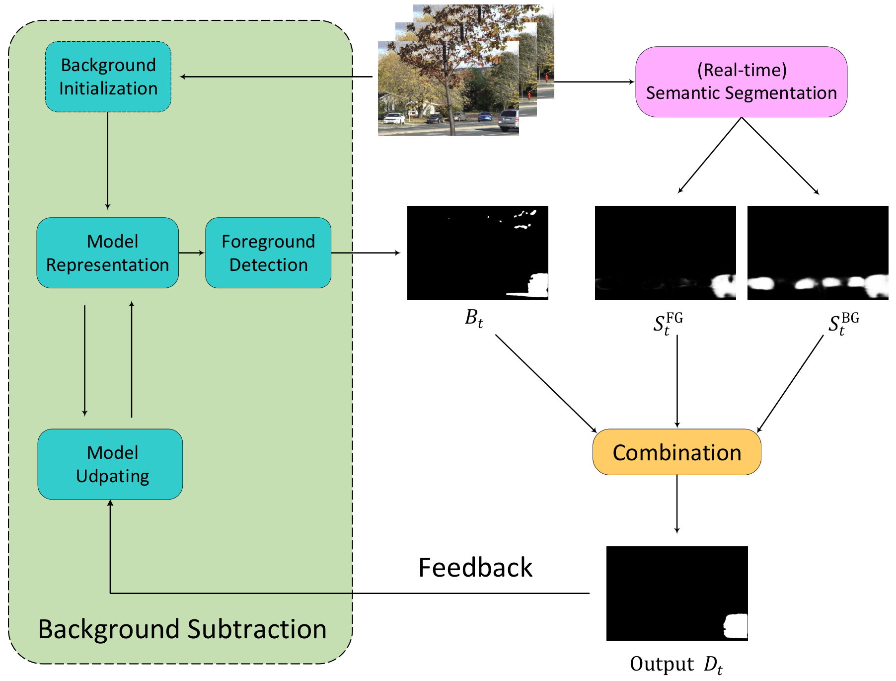
Through the above observations, we propose a novel background subtraction framework called background subtraction with real-time semantic segmentation (RTSS). The framework of our RTSS is illustrated in Fig. 1. The key idea is to decompose the original background subtraction into two parallel but collaborative components [19]: a traditional BGS segmenter and a real-time semantic segmenter . The BGS segmenter aims to construct background models and segments foreground objects. The semantic segmenter cooperates to refine the foreground segmentation result and feedback to improve the model updating accuracy. The BGS segmenter can be any real-time BGS algorithms. For semantic segmenter, in order to obtain real-time semantic information, we use two strategies. The first is to use real-time semantic segmentation algorithms, and the second is to perform semantic segmentation once every N frames. and work in parallel on two threads. For each input frame , the BGS segmenter performs the background subtraction process to produce a preliminary foreground/background (FG/BG) mask . At the same time, the real-time semantic segmenter segments object-level semantics . Then, some specific rules are applied on and and producing the final detection result . Finally, the refined FG/BG mask is fed back to update the background model. In contrast to [17], the proposed method can not only run in real time but also achieves higher detection precision due to the feedback mechanism.
We thus make the following contributions:
- 1.
We propose a novel background subtraction framework which combines traditional unsupervised BGS algorithms and real-time semantic segmentation algorithms. Experimental results show that RTSS achieved state-of-the-art performance among all unsupervised BGS methods while operating at real-time and even performs better than some deep learning based methods
- 2.
The proposed framework has a component based structure, allowing for flexibly replacing components and adaption to new applications.
The rest of this paper is organized as follows. Relevant work is discussed in Section II. Then in Section III, we elaborate the framework of RTSS. Section IV presents the experiments and comparisons with other state-of-the-art algorithms on the CDnet 2014 dataset [20]. Final conclusions are given in Section V.
II Related Works
Background subtraction and semantic segmentation have been extensively studied. A full survey is out of the scope of this paper. In the following we discuss some related works and refer readers to [1, 2, 52, 21] for a thorough review.
Background subtraction: Existing background subtraction algorithms can be categorized as traditional unsupervised algorithms and recent supervised algirithms which based on deep learning. The most popular and classic technology is the Gaussian Mixture Model (GMM) [3] which models the per-pixel distribution of gray values observed over time with a mixture of Gaussians. Since its introduction, GMM has been widely used in different scenarios and various improved versions have been proposed [4, 22]. However, GMM model presents some disadvantages. For example, when the background changes quickly, it is difficult to be modeled with just a few Gaussian models, and it may also fail to provide correct detections. To overcome these problems, a non-parametric approach using Kernel Density Estimation (KDE) technique was proposed in [6], which estimates the probability density function at each pixel from many samples without any prior assumptions. This model is robust and can adapt quickly to the background changes with small motions. A more advanced method using adaptive kernel density estimation was also proposed in [23]. The Codebook is another classic technology that has been introduced by Kim et al. in [7]. The values for each pixel are modeled into codebooks which represent a compressed form of background model in a long image sequence. Each codebook is composed of codewords constructed from intensity and temporal features. Incoming pixels matched against one of the codewords are classified as background; otherwise, foreground. The more recent ViBe algorithm [9] is built on similar principles as GMMs, but instead of building the probability distribution of the background pixels using a Parzen window, the authors try to store the distributions as a collection of samples at random. If a pixel in the new input frame matches a portion of its background samples, it is considered to be background and may be selected for model update. Local Binary Pattern (LBP) feature [15] is one of the earliest and popular texture operator proposed for background subtraction and has shown favourable performance due to its computational simplicity and tolerance against illumination variations. However, LBP is sensitive to subtle local texture changes caused by image noise. To deal with this problem, Tan et al. [24] proposed the Local Ternary Pattern (LTP) operator by adding a small tolerance offset. LTP is however not invariant to illumination variations with scale transform as the tolerance is constant for every pixel position. Recently, the Scale Invariant Local Ternary Pattern (SILTP) operator was proposed in [25] and has shown its robustness against illumination variations and local image noise within a range because it employs a scalable tolerance offset associated with the center pixel intensity. More recently, Local Binary Similarity Pattern (LBSP) was proposed by St-Charles et al. [16], this operator is based on absolute difference and is calculated both inside a region of an image and across regions between two images to take more spatiotemporal information into consideration. The authors also improved the method by combining LBSP features and pixel intensities with a pixel-level feedback loop model maintainance mechanism. The new method called SuBSENSE [10] achieves state-of-the-art performance among all traditional BGS algorithms.
In the past few years, many CNN-based background subtraction algorithms [26, 27, 28, 29, 30] have been proposed. The first scene specific CNN-based background subtraction method is proposed in [26]. First, a fixed background image is generated by a temporal median operation over the first 150 frames. Then, for each frame in a sequence, image patches centered on each pixel are extracted from the current frame and the background image. After that, the combined patches are fed to the network to get the probability of current pixel. After comparing with a score threshold, the pixel is either classified background or foreground. Babaee et al. [27] proposed a novel background image generation with a motion detector, which produces a more precise background image. Instead of training one network per scene, the authors collected 5% of frames from each sequence as the training data then trained only one model for all sequences. However, the precision of this algorithm is much worse than that of [26]. Wang et al. [28] proposed a multiscale cascade-like convolutional neural network architecture for background subtraction without constructing background images. More recently, Lim et al. [29] proposed an encoder-decoder type neural network with triplet CNN and transposed CNN configuration. Zeng et al. [30] proposed a multiscale fully convolutional network architecture which takes advantage of different layer features for background subtraction. Although the previous mentioned deep learning based algorithms perform better than the traditional algorithms, they all are supervised. During the training stage, ground truth constructed by a human expert or other unsupervised traditional BGS methods are needed to train their model. However, strictly speaking, background subtraction methods for video surveillance should be unsupervised. Therefore, it could be argued whether existing CNN-based background subtraction methods are useful in practical applications.
Semantic segmentation: Over the last years, development of convolutional neural networks has enabled remarkable progress in semantic segmentation. Early approaches performed pixel-wise classification by explicitly passing image patches through CNNs [31]. In [32], the fully convolutional network (FCN) proposed by Long et al. opened a new idea for semantic segmentation with end-to-end training. Transposed convolution operations are utilized to upsample low resolution features. This network architecture is far more efficient than pixel-wise prediction since it avoids redundant computation on overlapping patches. However, the typical FCN architectures involve a number of pooling layers to significantly increase the receptive field size and to make the network more robust against small translations. As a result, the network outputs are a low-resolution. To address this issue, various strategies have been proposed. Some approaches use dilated convolutions to augment the receptive field size without losing resolution [33, 34], extract features from different layers with skip-connections operation [35, 36], or multi-scale feature ensembles [37, 38]. Noh et al. [39] proposed an encoder-decoder structure. The encoder learns low-dimensional feature representations via pooling and convolution operations. While the decoder tries to upscale these low-dimensional features via a sequence of unpooling and deconvolution operations. In [34, 40], conditional random fields (CRFs) are applied on the network output in order to obtain more consistent results. Zhao et al. [18] proposed the pyramid scene network (PSPNet) for scene parsing by embedding difficult scenery context features, and achieved state-of-the-art performance on various semantic segmentation datasets.
All of the above mentioned segmentation approaches mainly focused on accuracy and robustness. Most of them are computationally expensive and cannot be applied in real-time applications. Recent interest in self-driving cars has created a strong need for real-time semantic segmentation algorithms. SegNet [41] tries to abandon layers to reduce network parameters to improve the network reference speed. LinkNet [43] presents an architecture that is based on residual connections, and Paszke et al. [42] proposed a lightweight residual network ENet by sacrificing layers to gain efficiency for real-time semantic segmentation. More recently, ERFNet [44] proposed a novel architecture with residual connections and factorized convolutions, which made a good trade-off between high accuracy and real-time speed. This system is able to run at 83 FPS for resolution image with an NVIDIA GTX Titan X GPU and achieves remarkable accuracy on various semantic segmentation datasets. ICNet [45] proposed a compressed-PSPNet-based image cascade network for pixel-wise label inference. Multi-resolution branches under proper label guidance are used to reduce network computational complexity. This real-time system can process resolution video stream at a speed of 30 fps while accomplishing acceptable segmentation precision.
III Background subtraction with real-time semantic segmentation
In this section, we will give a detailed description of the novel background subtraction framework RTSS (background subtraction with real-time semantic segmentation). The RTSS framework consists of two components: a BGS segmenter and a semantic segmenter . The and work together toward real-time and accuracy foreground detection. In this paper, we choose SuBSENSE [10] as the benchmark BGS segmenter and ICNet [45] as the benchmark semantic segmenter.
III-A SuBSENSE for Background Subtraction
We choose SuBSENSE [10] as the benchmark BGS segmenter as it shows state-of-the-art performance among all real-time unsupervised BGS algorithms. In the past few years, various non-parametric background subtraction methods have been proposed and have shown to outperform many existing methods. Barnich et al. [9] proposed the ViBe method whose background model is constructed by a collection of samples randomly selected over time. When a background sample is updated, its neighboring pixels also have a probability to update its background model according to the neighborhood diffusion strategy. Inspired by control system theory, Hofmann et al. [46] proposed an improved Vibe algorithm by dynamically adjusting the decision threshold and the learning rate. Then, St-Charles et al. proposed the SuBSENSE method [10], which combines color and local binary similarity pattern (LBSP) features to improve the spatial awareness and using a pixel-level feedback mechanism to dynamically adjust its parameters. A brief overview of SubSENSE is presented as follows. We define the background model at pixel as:
| (1) |
which contains recent background samples. To classify a pixel in the -th input frame as foreground or background, it will be matched against its background samples according to (2):
| (2) |
where is the output segmentation result, = 1 means foreground and = 0 means background. returns the distance between the input pixel and a background sample . is the distance threshold which can be dynamically changed for each pixel over time. If the distance between and is less than the threshold , a match is found. And is the minimum number of matches required for classifying a pixel as background, usually is fixed as 2.
To increase the model robustness and flexibility, the distance threshold need to be dynamically adjusted per-pixel. A feedback mechanism based on two-pronged background monitoring is proposed. First, to measure the motion entropy of dynamic background, a new controller is defined:
| (3) |
where is the minimal normalized distance, and is the learning rate. For dynamic background region pixels, trends to the value 1, and for static background regions, trends to 0. Then, a pixel-level accumulator is defined to monitor blinking pixels:
| (4) |
where and are two fixed parameters with the value of 1 and 0.1, respectively. is the blinking pixel map calculated by an XOR operation between and . With and defined, the distance threshold can be recursively adjusted as follows:
| (5) |
The background update rate parameter is used to control the speed of the background absorption. The randomly-picked background samples in have the probability of to be replaced by , if current pixel belongs to the background. The lower the is, the higher the update probability, and vice versa. is also recursively adjusted by and . More specifically, is defined as follows:
| (6) |
The authors also define a lower bound and an upper bound to clamp to the interval .
III-B ICNet for Real-time Semantic Segmentation
We adopt ICNet [45] to develop the benchmark semantic segmenter . The ICNet achieved an excellent trade-off between efficiency and accuracy for real-time semantic segmentation. To reduce network computational complexity, a multi-resolution cascade network architecture was proposed. Its core idea is to let the low-resolution image go through the full semantic network first for a coarse segmentation map. Then, a cascade fusion unit introduces middle- and high-resolution image feature to help improving the coarse segmentation map gradually.
In order to extract object-level potential foreground semantic information for the Change Detection dataset sequences [20], we first train an ICNet model for semantic segmentation with the ADE20K dataset [47]. The ADE20K dataset is a recently released benchmark for scene parsing. It contains 20K/2K/3K high quality pixel-level annotations images for training, validation and testing. The pixel annotations span 150 classes (e.g., person, car, and tree) which frequently occur in diverse scenes. Therefore, it covers a large number of object categories and scene distributions. Here, we define to be the set of object classes.
After the training process, the trained model is executed on the Change Detection dataset sequences. However, before feeding a frame through the network, we need to make some padding around the image so that it can adapt to the input structure of the network since sequences from the Change Detection dataset have a variety of sizes. After the forward pass, the last layer of the model outputs a real value in each pixel for each of the object classes. We denote the real value vector of pixel at -th frame for all classes as: , where is the predict score for class . Then, a softmax function is applied on to get the probability vector with denotes the probability for class . However, since we want to get potential foreground object information for background subtraction problems, only a subset classes from the 150 labels are relevant. The same with [17], we choose the semantic relevant foreground classes as: {person, car, cushion, box, book, boat, bus, truck, bottle, van, bag, bicycle} , which are the most frequent foreground objects appeared in the Change Detection dataset. Finally, we compute the semantic foreground probability map as follows (mapping to 0255):
| (7) |
Fig. 2 shows some semantic foreground segmentation results on the Change Detection dataset sequences.

III-C RTSS Framework

After introducing the benchmark BGS segmenter and the semantic segmenter , we will give a detailed description of how and cooperate together for real-time and accuracy foreground detection. Fig. 3 illustrates the proposed RTSS (background subtraction with real-time semantic segmentation) framework.
In RTSS, and run in parallel on two synchronous threads while collaborating with each other. The BGS segmenter is mainly responsible for the background subtraction process and the semantic segmenter is employed to detect the object-level potential foreground object(s). For each input frame, in the BGS segmenter thread, performs the BG/FG classification process. At the same time, in the semantic segmenter thread, makes the semantic segmentation process. As we mentioned before, in order to obtain real-time semantic information, we have two strategies to choose from. The first one is to use real-time semantic segmentation algorithms such as ICNet [45], ERFNet [44], LinkNet [43], and so on. The second one is to present the semantic segmentation operation once every N (N 1) frames if the semantic segmentation algorithms cannot run in real time. The reason behind this is that in most cases, two consecutive frames in a video are highly redundant, the semantic segmentation results in two adjacent frames may be very similar, the extracted potential foreground objects may only have small displacements. In Fig. 3, for the semantic segmenter , if a real-time semantic segmentation algorithm is used, then, N is set to 1. That is to say, every input frame is semantically segmented. If a non-real-time semantic segmentation algorithm is used, then, N is set to a number greater than 1. That is to say, we do the semantic segmentation every N frames. More specifically, suppose the current frame is the t-th input frame, and semantic segmentation is performed to get the semantic foreground probability map . However, we will then skip the semantic segmentation operation on the frames, but use as an alternative semantic foreground probability map of these frames. In this way, the computational time of the semantic segmenter can be greatly reduced.
The collaboration process between and can be summarized as Algorithm 1. When an input frame is available, in the thread, it runs the BGS algorithm to do the foreground detection first, and gets a preliminary foreground/background (FG/BG) mask . At the same time, in the semantic segmenter thread , it forwards to the trained model and uses the output result to calculate the semantic foreground probability map , then, trigger a signal that is available. On the other side, in the thread, after the foreground detection process is finished, it will wait until is available. Once is available, the BGS segmenter will combine and to produce a more precise FG/BG mask . Finally, the refined FG/BG mask is fed back to update the background model. Go to the next frame and repeat the process until all the frames are processed.
Fig. 4 presents the interaction process between the SuBSENSE [10] algorithm and semantic segmentation algorithm. is the current input frame, , , , and are internal parameters of SuBSENSE as shown in III-A. and are the foreground detection and semantic segmentation results of current frame, respectively. After and are obtained, some specific rules are applied on and to get a more precise FG/BG mask . At the same time, the refined FG/BG mask is fed back into the background subtraction process and guide the background model updating, which produces a more reliable background model. As time goes by, the accuracy of foreground detection result in SuBSENSE can be greatly improved, and finally made the final result better and better.
Now, the remaining key problem is how can we make use of the semantic foreground segmentation result to compensate for the errors of the background subtraction result and to produce a more accurate result . In this work, we use a similar strategy presented in [17]. First, we want to extract two useful information from the semantic foreground segmentation . One is to point out which pixels have high confidence that belong to the background. The other one shows which pixels have a higher probability of belonging to foreground. We denote them as and respectively. In this work, we define as follows:
| (8) |
While for , it is defined as follows:
| (9) |
where is regarded as a semantic background model for pixel at time . Firstly, is initialized in the first frame with . Then, to keep the adaptation of the model to the scene changes, a conservative random updating strategy as introduced in [9] is adopted to update . More specifically, if is classified as FG, remains unchanged; if is classified as BG, has a probability of to be updated by , where is a time subsampling factor which controls the adaptation speed. This conservative updating strategy can avoid model corruption due to intermittent and slow moving foreground objects. This process can be summarized by Algorithm 2:
Fig. 5 shows some examples of background subtraction result , and semantic segmentation results and on the Change Detection dataset sequences.

We now need to define some rules for combining , and to get .
Firstly, we specify that pixels with a low semantic foreground probability in should be classified as background without considering , as shown as follows:
| (10) |
where is the threshold value for background. As shown in Fig. 5, the BGS segmenter produces many false positive pixels due to dynamic backgrounds, illumination variations and shadows, which severely affect the accuracy of the foreground detection result. However, rule (10) provides a simple way to address these challenges.
Secondly, pixels with a high semantic foreground probability in should be classified as foreground, as shown as follows:
| (11) |
where denotes the threshold value for the foreground. rule (11) is mainly focused on correcting false negative detection pixels. In Fig. 5, we can see that when foreground samples and background model share similar features due to camouflage or model absorption, many “holes” appear in foreground object, while can be used to compensate and correct these errors.
Finally, if all the previous conditions are not satisfied, this means that the semantic segmentation result cannot provide enough information to make a decision. At this time, we directly take the BGS algorithm result as the final result with . To sum up, the complete , and combination process can be summarized with Equation (12):
| (12) |
IV Experimental Results
In this section, we first give a brief introduction of evaluation dataset and metrics. Then we provide both quantitative and qualitative comparisons with state-of-the-art background subtraction methods. We also perform an ablation study of the RTSS framework.
IV-A Evaluation Dataset and Metrics
We evaluate the performance of the proposed RTSS framework for background subtraction using the Change Detection (CDnet) 2014 dataset [20]. The CDnet 2014 dataset is a region-level benchmark obtained from realistic scenarios. Accurate human experts constructed ground truths are available for all sequences. This dataset contains 53 video sequences which are grouped into 11 different video categories comprising “baseline”, “camera jitter”, “dynamic background”, “intermittent object motion”, “shadow”, “thermal”, “bad weather”, “low framerate”, “night videos”, “pan-tilt-zoom” and “turbulence”. The resolution of the sequences varies from to with hundred to thousand frames. To our knowledge, this is one of the most comprehensive datasets for background subtraction evaluations.
To make an exhaustive quantitative comparison between different background subtraction methods, seven different quantitative metrics have been defined in [20]: Recall (Re), Specificity (Sp), False positive rate (FPR), False negative rate (FNR), Percentage of wrong classifications (PWC), Precision (Pr), F-Measure (FM).
All these metric values range from 0 to 1. For Re, Sp, Pr and FM metrics, higher values indicate more accuracy while for PWC, FNR and FPR metrics, lower values indicate better performance.
All the measured metrics depend on TP (True Positives), TN (True Negatives), FP (False Positives), and FN (False Negatives). TP is the correctly detected foreground pixels, TN is the correctly detected background pixels, FP is the number of background pixels detected as foreground and FN is the number of foreground pixels detected as background.
• Recall (Re) =
• Specificity (Sp) =
• False positive rate (FPR) =
• False negative rate (FNR) =
• Percentage of wrong classifications (PWC) =
• Precision (Pr) =
• F-Measure (FM) =
Generally speaking, a background subtraction method is considered good if it gets high recall scores, without sacrificing precision. Therefore, the F-Measure (FM) metric which represents a balance between the Recall and Precision, is mainly accepted as a single indicator of the overall performance of different BGS methods.
IV-B Parameter Setting
As discussed above, the proposed method contains a few parameters which should be determined before building a complete model: the threshold for background , the threshold for foreground and the time subsampling factor . The performance with different parameter settings are show in Fig. 6. Although we can obtain optimal performance by adjusting parameters in different scenarios, we used a universal parameter set for all sequences to respect the competition rules of the Change Detection dataset [20].
| Category | Recall | Specificity | FPR | FNR | PWC | Precision | F-Measure |
|---|---|---|---|---|---|---|---|
| baseline | 0.9519(0.9566 ) | 0.9982(0.9946 ) | 0.0018(0.0054 ) | 0.0481(0.0434 ) | 0.3639(0.6310 ) | 0.9486(0.9093 ) | 0.9498(0.9312 ) |
| cameraJ | 0.8319(0.8131 ) | 0.9901(0.9914 ) | 0.0099(0.0086 ) | 0.1681(0.1869 ) | 1.6937(1.6788 ) | 0.7944(0.8193 ) | 0.8096(0.7995 ) |
| dynamic | 0.7739(0.9191 ) | 0.9994(0.9992 ) | 0.0006(0.0008 ) | 0.2261(0.0809 ) | 0.4094(0.1544 ) | 0.8913(0.8980 ) | 0.8159(0.9053 ) |
| intermittent | 0.5715(0.7354 ) | 0.9953(0.9963 ) | 0.0047(0.0037 ) | 0.4285(0.2646 ) | 4.0811(3.0055 ) | 0.8174(0.8841 ) | 0.6068(0.7802 ) |
| shadow | 0.9441(0.9590 ) | 0.9920(0.9942 ) | 0.0080(0.0058 ) | 0.0559(0.0410 ) | 1.0018(0.7243 ) | 0.8645(0.8938 ) | 0.8995(0.9242 ) |
| thermal | 0.8166(0.6492 ) | 0.9910(0.9903 ) | 0.0090(0.0097 ) | 0.1834(0.3508 ) | 1.9632(2.4733 ) | 0.8319(0.8626 ) | 0.8172(0.7007 ) |
| badWeather | 0.8082(0.7442 ) | 0.9991(0.9993 ) | 0.0009(0.0007 ) | 0.1918(0.2558 ) | 0.4807(0.5061 ) | 0.9183(0.9504 ) | 0.8577(0.8196 ) |
| lowFramerate | 0.8267(0.8050 ) | 0.9937(0.9952 ) | 0.0063(0.0048 ) | 0.1733(0.1950 ) | 1.2054(1.1464 ) | 0.6475(0.6787 ) | 0.6659(0.6849 ) |
| nightVideos | 0.5896(0.5341 ) | 0.9837(0.9879 ) | 0.0163(0.0121 ) | 0.4104(0.4659 ) | 2.5053(2.1386 ) | 0.4619(0.5244 ) | 0.4895(0.4933 ) |
| PTZ | 0.8293(0.8713 ) | 0.9649(0.9865 ) | 0.0351(0.0135 ) | 0.1707(0.1287 ) | 3.6426(1.4582 ) | 0.3163(0.4157 ) | 0.3806(0.5158 ) |
| turbulence | 0.8213(0.8423 ) | 0.9998(0.9996 ) | 0.0002(0.0004 ) | 0.1787(0.1577 ) | 0.1373(0.1352 ) | 0.9318(0.8788 ) | 0.8689(0.8590 ) |
| Overall | 0.7968(0.8027 ) | 0.9916(0.9940 ) | 0.0084(0.0060 ) | 0.2032(0.1973 ) | 1.5895(1.2774 ) | 0.7658(0.7923 ) | 0.7420(0.7649 ) |
- 1
Note that blue entries indicate the original SuBSENSE results. In parentheses, the purple entries indicate the RTSS results, and the arrows show the variation when compared to the original SuBSENSE results.
| Category | Recall | Specificity | FPR | FNR | PWC | Precision | F-Measure |
|---|---|---|---|---|---|---|---|
| baseline | 0.9519(0.9659 ) | 0.9982(0.9979 ) | 0.0018(0.0021 ) | 0.0481(0.0341 ) | 0.3639(0.3119 ) | 0.9486(0.9552 ) | 0.9498(0.9603 ) |
| cameraJ | 0.8319(0.8284 ) | 0.9901(0.9936 ) | 0.0099(0.0064 ) | 0.1681(0.1716 ) | 1.6937(1.3762 ) | 0.7944(0.8780 ) | 0.8096(0.8395 ) |
| dynamic | 0.7739(0.9273 ) | 0.9994(0.9994 ) | 0.0006(0.0006 ) | 0.2261(0.0727 ) | 0.4094(0.1293 ) | 0.8913(0.9390 ) | 0.8159(0.9328 ) |
| intermittent | 0.5715(0.7473 ) | 0.9953(0.9975 ) | 0.0047(0.0025 ) | 0.4285(0.2527 ) | 4.0811(2.8421 ) | 0.8174(0.9026 ) | 0.6068(0.7938 ) |
| shadow | 0.9441(0.9681 ) | 0.9920(0.9972 ) | 0.0080(0.0028 ) | 0.0559(0.0319 ) | 1.0018(0.3999 ) | 0.8645(0.9441 ) | 0.8995(0.9557 ) |
| thermal | 0.8166(0.8489 ) | 0.9910(0.9907 ) | 0.0090(0.0093 ) | 0.1834(0.1511 ) | 1.9632(1.4590 ) | 0.8319(0.8559 ) | 0.8172(0.8499 ) |
| badWeather | 0.8082(0.8028 ) | 0.9991(0.9994 ) | 0.0009(0.0006 ) | 0.1918(0.1972 ) | 0.4807(0.4314 ) | 0.9183(0.9475 ) | 0.8577(0.8657 ) |
| lowFramerate | 0.8267(0.8224 ) | 0.9937(0.9956 ) | 0.0063(0.0044 ) | 0.1733(0.1776 ) | 1.2054(1.0276 ) | 0.6475(0.6861 ) | 0.6659(0.6970 ) |
| nightVideos | 0.5896(0.4710 ) | 0.9837(0.9916 ) | 0.0163(0.0084 ) | 0.4104(0.5290 ) | 2.5053(1.9308 ) | 0.4619(0.6068 ) | 0.4895(0.4868 ) |
| PTZ | 0.8293(0.8735 ) | 0.9649(0.9917 ) | 0.0351(0.0083 ) | 0.1707(0.1265 ) | 3.6426(0.9339 ) | 0.3163(0.5349 ) | 0.3806(0.6323 ) |
| turbulence | 0.8213(0.8528 ) | 0.9998(0.9994 ) | 0.0002(0.0006 ) | 0.1787(0.1472 ) | 0.1373(0.1579 ) | 0.9318(0.8102 ) | 0.8689(0.8191 ) |
| Overall | 0.7968(0.8280 ) | 0.9916(0.9958 ) | 0.0084(0.0042 ) | 0.2032(0.1720 ) | 1.5895(1.0000 ) | 0.7658(0.8237 ) | 0.7420(0.8030 ) |
- 1
Note that blue entries indicate the original SuBSENSE results. In parentheses, the purple entries indicate the RTSS results, and the arrows show the variation when compared to the original SuBSENSE results.
| Method | Overall | |||||||||||
|---|---|---|---|---|---|---|---|---|---|---|---|---|
| ERFNet | 0.7570 | 0.9549 | 0.8104 | 0.8908 | 0.7708 | 0.9297 | 0.6298 | 0.8474 | 0.6728 | 0.5276 | 0.4965 | 0.7989 |
| LinkNet | 0.7593 | 0.9541 | 0.8118 | 0.8532 | 0.7203 | 0.9145 | 0.7548 | 0.8627 | 0.6869 | 0.5052 | 0.4610 | 0.8278 |
| PSPNet | 0.7755 | 0.9526 | 0.8178 | 0.9263 | 0.7892 | 0.9394 | 0.8496 | 0.8544 | 0.5958 | 0.4615 | 0.5477 | 0.7962 |
| PSPNet | 0.7892 | 0.9574 | 0.8345 | 0.9322 | 0.7929 | 0.9500 | 0.8488 | 0.8628 | 0.6249 | 0.4741 | 0.5917 | 0.8120 |
| MFCN | 0.9570 | 0.9798 | 0.9740 | 0.9781 | 0.9385 | 0.9859 | 0.9699 | 0.9693 | 0.9048 | 0.9173 | 0.9516 | 0.9582 |
IV-C Ablation Analysis
| Method | Recall | Specificity | FPR | FNR | PWC | Precision | F-Measure |
|---|---|---|---|---|---|---|---|
| GMM [3] | 0.6195 | 0.9870 | 0.0130 | 0.3805 | 2.9030 | 0.6171 | 0.5390 |
| RTSS | 0.6792 | 0.9920 | 0.0080 | 0.3208 | 2.0622 | 0.6992 | 0.6302 () |
| RTSS | 0.7146 | 0.9948 | 0.0052 | 0.2854 | 1.6941 | 0.7517 | 0.6957 () |
| ViBe [9] | 0.6146 | 0.9738 | 0.0262 | 0.3854 | 3.8341 | 0.6614 | 0.5761 |
| RTSS | 0.6465 | 0.9882 | 0.0118 | 0.3535 | 2.2954 | 0.7210 | 0.6307 () |
| RTSS | 0.6872 | 0.9940 | 0.0060 | 0.3128 | 1.5994 | 0.7789 | 0.6978 () |
| PBAS [46] | 0.7268 | 0.9542 | 0.0458 | 0.2732 | 5.2080 | 0.7019 | 0.6426 |
| RTSS | 0.7265 | 0.9824 | 0.0176 | 0.2735 | 2.4598 | 0.7327 | 0.6733 () |
| RTSS | 0.7630 | 0.9914 | 0.0086 | 0.2370 | 1.4363 | 0.7925 | 0.7411 () |
Ablation study for semantic segmentation algorithms: In Table I, we present the complete quantitative evaluation results of the proposed method on the CDnet 2014 dataset, seven metrics and overall scores are reported. The blue entries indicate the original SuBSENSE results, while the proposed RTSS framework which combines SuBSENSE and ICNet (RTSS) results are shown in the parentheses with purple entries. The arrows indicate the variations between the two. We can see that RTSS achieves an over F-Measure score of 0.7649, which is a 3% improvement compared to the original SuBSENSE. This improvement is mainly benefited from “dynamic background”, “intermittent object motion”, “shadow”, “low framerate”, and “pan-tilt-zoom” categories. The dynamic background category contains six challenging videos depicting outdoor scenarios, where there is dynamic motion in the background such as trees shaking in the wind, boats moving on the river and cars passing behind rippling fountains. However, RTSS improves the F-Measure by a significant margin of 11% on this category, which demonstrates its tolerance for dealing with background changes. The intermittent object motion category includes six videos, each of which contains objects with intermittent motion such as parked cars suddenly start moving and objects are abandoned, which resulting ghost artifacts in the detected result. Due to the object-level semantic information provided by the semantic segmenter , the proposed method has a remarkable 29% improvement on the F-Measure score. The same can be said for the pan-tilt-zoom (PTZ) category, which contains videos captured with moving camera, making it hard for most algorithms to adapt to the scene changes. Due to the use of potential foreground semantic segmentation, the proposed method can distinguish the potential foreground and background information quickly despite camera motions, which makes an amazing 36% improvement for this category. For the shadow category which comprised videos exhibiting shadows and reflections and the low framerate category which included four outdoor videos with the frame rate varies from 0.17 to 1 FPS, RTSS also has a 3% improvement of the F-Measure score.
However, from Table I, we can also find that in some categories such as baseline, camera jitter, thermal, bad weather and turbulence, compared to the original SuBSENSE, RTSS performs worse than the original algorithm. Our hypothesis is that the precision of the semantic segmenter is not accurate enough. Because similar phenomena can be found when other real-time semantic segmentation algorithms are used, such as ERFNet [44], LinkNet [43], as shown in Table III (more complete and detailed results are reported in Appendix). Therefore, we introduce the state-of-the-art semantic segmentation method PSPNet into the RTSS framework to replace the ICNet. We call the new algorithm RTSS, repeat the same experimental process as before, and the final results are shown in Table II, which illustrates that our hypothesis seems correct.
We can see that RTSS achieves an overall F-Measure of 0.8030 on the whole dataset, about 8% improvement compared to the 3% of RTSS, which is a significant margin. In addition to the night videos and turbulence categories, all the remaining categories have a significant performance improvement especially in the dynamic background, intermittent object motion, shadow and PTZ categories. The trend of these performance improvements is consistent with the RTSS results. In the turbulence category, the videos are captured with long distance thermal lens. The most prominent characteristic of this category is that the sequences suffer from air turbulence under high temperature environments, which resulting distortion in each frame. Since the semantic segmentation network model is trained on the ADE20K dataset [47], images from the turbulence category have a big difference with the ADE20K dataset, thus the semantic foreground/background segmentation for these sequences are unstable and inaccurate. So we can see that both RTSS and RTSS have the F-Measure decrease in this category. If the semantic segmenter can provide more accuracy semantic information, we may get better results. However, we should also notice that the high computational complexity of PSPNet makes it difficult to achieve real-time performance if we perform semantic segmentation for every frame in the RTSS framework. So, as we mentioned before, consecutive frames in a video are highly redundant, we can do the semantic segmentation every N frames. Table III shows the results of PSPNet with N = 2 and N = 3 (more complete and detailed results are reported in Appendix). Although their results are not as good as N = 1, they also show a big improvement compared with the original SuBSENSE.
Finally, we use a deep learning-based supervised BGS algorithm MFCN [30] as the semantic segmenter (since we cannot get a more precise semantic segmentation algorithm than PSPNet at present). For each sequence in the CDnet 2014 dataset, a subset of 200 input frames with their corresponding ground truths is randomly and manually selected to train the model. Then we take the output of MFCN on each frame as the semantic information. Repeat the same experimental process as before, we get an overall F-Measure of 0.9570, this again verifies our speculations.
Ablation study for BGS algorithms: We now make an ablation study for BGS algorithms on the proposed RTSS framework. Three classic BGS algorithms GMM [3], ViBe [9] and PBAS [46] are introduced into the RTSS framework to replace SuBSENSE. We report the experimental results in Table IV. The blue entries indicate the original BGS algorithm results, the purple entries indicate the RTSS results, and the arrows show the F-Measure variation when compared to the original algorithm. We can see that all of them have a remarkable improvement when compared with their original BGS algorithms. The RTSS which combines GMM and ICNet improves from 0.5390 to 0.6302, about 17% F-Measure improvement, and RTSS is about 9%, RTSS is about 5%. When more accurate semantic segmentation algorithm is used, the promotion effect is more obvious, we can find that RTSS, RTSS, RTSS have 29%, 21%, 15% promotion, respectively.
Based on above analysis, we can find that the proposed RTSS framework is very flexible, and can be applied to many BGS algorithms. The choices of BGS segmenter and semantic segmenter may depend on application scenarios and computational resources. We also believe that the proposed framework has great potential for future improvement with the emergence of faster and more accurate BGS algorithms and semantic segmentation algorithms.
| Method | Recall | Specificity | FPR | FNR | PWC | Precision | F-Measure |
|---|---|---|---|---|---|---|---|
| SuBSENSE [10] | 0.7968 | 0.9916 | 0.0084 | 0.2032 | 1.5895 | 0.7658 | 0.7420 |
| SemanticBGS | 0.7797 | 0.9939 | 0.0061 | 0.2203 | 1.4529 | 0.7862 | 0.7490 () |
| RTSS | 0.8027 | 0.9940 | 0.0060 | 0.1973 | 1.2774 | 0.7923 | 0.7649 () |
| SemanticBGS | 0.8079 | 0.9955 | 0.0045 | 0.1926 | 1.1294 | 0.8153 | 0.7874 () |
| RTSS | 0.8280 | 0.9958 | 0.0042 | 0.1720 | 1.0000 | 0.8237 | 0.8030 () |
| Method | Overall | |||||||||||
|---|---|---|---|---|---|---|---|---|---|---|---|---|
| FgSegNet [29] | 0.9770 | 0.9973 | 0.9954 | 0.9958 | 0.9951 | 0.9937 | 0.9921 | 0.9845 | 0.8786 | 0.9655 | 0.9843 | 0.9648 |
| CascadeCNN [28] | 0.9209 | 0.9786 | 0.9758 | 0.9658 | 0.8505 | 0.9593 | 0.8958 | 0.9431 | 0.8370 | 0.8965 | 0.9168 | 0.9108 |
| RTSS | 0.7917 | 0.9597 | 0.8396 | 0.9325 | 0.7864 | 0.9551 | 0.8510 | 0.8662 | 0.6771 | 0.5295 | 0.5489 | 0.7630 |
| IUTIS-5 [48] | 0.7717 | 0.9567 | 0.8332 | 0.8902 | 0.7296 | 0.8766 | 0.8303 | 0.8248 | 0.7743 | 0.5290 | 0.4282 | 0.7836 |
| RTSS | 0.7571 | 0.9312 | 0.7995 | 0.9053 | 0.7802 | 0.9242 | 0.7007 | 0.8454 | 0.6643 | 0.5479 | 0.4324 | 0.7969 |
| RTSS | 0.7502 | 0.9541 | 0.8118 | 0.8532 | 0.7203 | 0.9145 | 0.7548 | 0.8612 | 0.6687 | 0.5480 | 0.3911 | 0.7744 |
| SharedModel [49] | 0.7474 | 0.9522 | 0.8141 | 0.8222 | 0.6727 | 0.8898 | 0.8319 | 0.8480 | 0.7286 | 0.5419 | 0.3860 | 0.7339 |
| DeepBS [27] | 0.7458 | 0.9580 | 0.8990 | 0.8761 | 0.6098 | 0.9304 | 0.7583 | 0.8301 | 0.6002 | 0.5835 | 0.3133 | 0.8455 |
| RTSS | 0.7450 | 0.9549 | 0.8104 | 0.8908 | 0.7708 | 0.9276 | 0.6298 | 0.8457 | 0.6512 | 0.5455 | 0.4151 | 0.7528 |
| WeSamBE [50] | 0.7446 | 0.9413 | 0.7976 | 0.7440 | 0.7392 | 0.8999 | 0.7962 | 0.8608 | 0.6602 | 0.5929 | 0.3844 | 0.7737 |
| SuBSENSE [10] | 0.7408 | 0.9503 | 0.8152 | 0.8177 | 0.6569 | 0.8986 | 0.8171 | 0.8619 | 0.6445 | 0.5599 | 0.3476 | 0.7792 |
| PAWCS [11] | 0.7403 | 0.9397 | 0.8137 | 0.8938 | 0.7764 | 0.8913 | 0.8324 | 0.8152 | 0.6588 | 0.4152 | 0.4615 | 0.6450 |
| C-EFIC [51] | 0.7307 | 0.9309 | 0.8248 | 0.5627 | 0.6229 | 0.8778 | 0.8349 | 0.7867 | 0.6806 | 0.6677 | 0.6207 | 0.6275 |
- 1
The methods in blue color are the unsupervised BGS methods, like ours. For completeness, we also show in orange color the supervised BGS methods.
IV-D Comparisons with State-of-the-art Methods
Quantitative Evaluation: Firstly, to demonstrate one of our key contribution, the proposed RTSS framework is preferable to the method presented in [17] by taking a semantic segmentation as a post-processing operation to refine the BGS segmentation result (we call this algorithm SemanticBGS), in Table V, we present the performance comparison results. The first row shows the seven metric results of the original SuBSENSE BGS algorithm, the second row gives the comparison results of SemanticBGS and RTSS when cooperated with the ICNet [45] semantic segmentor, and the third row shows the results when using the PSPNet [18]. For a specific metric, if the method obtains a better performance, the corresponding value is highlighted in bold. From Table V, we can see that the proposed method RTSS surpasses the SemanticBGS method on all seven metrics. The overall F-Measure score of SemanticBGS is only with nearly 1% improvement compared with the proposed RTSS of 3%. When combined with the PSPNet, the SemanticBGS has a 6% promotion while RTSS obtains 8% improvement, the gap is obvious. Therefore, this fully demonstrates the effectiveness of the algorithm proposed in this paper, that is, feeding back the refined FG/BG mask produced by the BGS segmenter and semantic segmenter to the background subtraction process to guide the background model updating can significantly improve the final accuracy.
We also compare our proposed method with other state-of-the-art algorithms listed on www.changedetection.net. In Table VI, we give a detailed overall and per-category F-Measure comparison, as well as the average ranking. The results are reported by the online evaluation server11 1 http://jacarini.dinf.usherbrooke.ca/results2014/589/ (589-592). For some sequences in the CDnet 2014 dataset, their ground truths are not public available, so the local evaluation results presented in the previous tables may have some difference with the online server reported results.. Due to space limitation, we only show the top-ranked methods: FgSegNet [29], CascadeCNN [28], IUTIS-5 [48], SharedModel [49], DeepBS [27], WeSamBE [50], SuBSENSE [10], PAWCS [11] and C-EFIC [51]. Among them, FgSegNet, CascadeCNN and DeepBS are deep learning based supervised methods. Since IUTIS involves a training process with ground truths, here, we also regard it as a supervised method. In Table VI, these supervised methods are marked with orange and the unsupervised ones with blue. Firstly, it can be observed that the top two methods are all deep learning based, FgSegNet even achieves an overall F-Measure of 0.9770, which is much higher than the proposed RTSS algorithms. However, as we stated earlier, from the point of view of applications, BGS algorithms for video surveillance should be unsupervised. Therefore, it could be argued whether these algorithms can be applied to scenarios like the ones we consider in this paper. Secondly, we can see that the proposed RTSS framework achieves state-of-the-art performance among all unsupervised methods and in fact even performs better than some deep learning based method such as DeepBS. It is worth noting that RTSS is a very flexible framework, allowing for easy changing the components if required.
Qualitative evaluation: Visual comparison of the foreground segmentation results are reported with 6 challenging sequences from the CDnet 2014 dataset [20]: highway ( = 818) from the “baseline” category, boulevard ( = 2318) from the “camera jitter” category, boats ( = 7914) from the “dynamic background” category, sofa ( = 1169) from the “intermittent object motion” category, peopleInShade ( = 1098) from the “shadow” category and continuousPan ( = 989) from the “pan-tilt-zoom” category. Fig. 7 provides qualitative comparison results with different methods. Visually, we can see that the results of the proposed RTSS method look much better than the corresponding baseline method, which shows good agreement with above quantitative evaluation results.
In the highway and boats sequences, which contain dynamic backgrounds such as tree branches moving with the wind and rippling water in the river, the proposed method can extract complete foreground objects and shows good robustness to the background disturbance. In the boulevard sequences, due to the repetitive jitter of the camera, many false positives are produced by other BGS methods. However, our foreground detection result is very accurate and complete. In the sofa sequence, which contains challenge about intermittent object motion, many false negatives are produced by other methods due to model absorption, but we can see that the proposed method performs well. In the peopleInShade sequence from the “shadow” category, we can find that although the shadow is strong, it only has a small impact on our results. In the continuousPan, although the camera is not static, RTSS also detects cars perfectly and shows good robustness for the motion background. All the above analysis again demonstrates the effectiveness of the proposed RTSS in variety challenging situations.
IV-E Processing Speed
We know that background subtraction is often the first step in many computer vision applications. Processing speed is a critical factor. In order to analyze the computational cost of the proposed method, we report the processing time of our method runs on the highway () sequence. The results are shown in Table VII. The experiment is performed on a computer with an Intel Core-i7 8700K processor with 32 GB memory and an NVIDIA Titan Xp GPU. The operating system is Ubuntu 16.04. We do not consider I/O time. According to the results, we can see that the average processing time of RTSS is about 38 ms per frame, which shows real-time performance. If we use the more accurate PSPNet, the average processing time is about 51 ms per frame with N = 3. However, the flexibility of the proposed RTSS framework allows the inclusion of faster and more accurate semantic segmentation algorithms, once they emerged.
| RTSS | RTSS |
| 38 | 51 |

V Conclusion
We proposed a novel background subtraction framework called background subtraction with real-time semantic segmentation (RTSS), which consists of two components: a BGS segmenter and a semantic segmenter , which work in parallel on two threads interactively for real-time and accurate foreground segmentation. Experimental results obtained on the CDnet 2014 dataset demonstrated the effectiveness of the proposed algorithm. Compared to other background subtraction methods, our method achieves state-of-the-art performance among all unsupervised background subtraction methods while operating at real-time, and even performs better than some deep learning based supervised algorithms. Moreover, it is worth noting that the proposed framework is very flexible, allowing for both easy adaption of future segmentation improvements and application driven component changes.
A number of improvements can be considered for our method. Our future work will focus on more efficient fusion strategy between the outputs of semantic segmentation and background subtraction, as well as more accurate and faster BGS and semantic segmentation algorithms.
Acknowledgment
This research is supported by the National Science Foundation of China under Grant No.61401425. We gratefully acknowledge the support of NVIDIA Corporation with the donation of the Titan Xp GPU used for this research.
Appendix
References
- [1] T. Bouwmans, “Traditional and recent approaches in background modeling for foreground detection: An overview,” Comput. Sci. Rev., vol. 11, pp. 31–66, 2014.
- [2] A. Sobral and A. Vacavant, “A comprehensive review of background subtraction algorithms evaluated with synthetic and real videos,” Comput. Vision Image Understanding, vol. 122, pp. 4–21, 2014.
- [3] C. Stauffer and W. E. L. Grimson, “Adaptive background mixture models for real-time tracking,” in Proc. IEEE Conf. Comput. Vis. Pattern Recognit., vol. 2. IEEE, 1999, pp. 246–252.
- [4] Z. Zivkovic and F. Van Der Heijden, “Efficient adaptive density estimation per image pixel for the task of background subtraction,” Pattern Recognit. Lett., vol. 27, no. 7, pp. 773–780, 2006.
- [5] M. S. Allili, N. Bouguila, and D. Ziou, “A robust video foreground segmentation by using generalized gaussian mixture modeling,” in Proc. IEEE Int. Conf. Comput. Robot Vis. IEEE, 2007, pp. 503–509.
- [6] A. Elgammal, R. Duraiswami, D. Harwood, and L. S. Davis, “Background and foreground modeling using nonparametric kernel density estimation for visual surveillance,” Proc. IEEE, vol. 90, no. 7, pp. 1151–1163, 2002.
- [7] K. Kim, T. H. Chalidabhongse, D. Harwood, and L. Davis, “Real-time foreground–background segmentation using codebook model,” Real-time Imaging, vol. 11, no. 3, pp. 172–185, 2005.
- [8] J.-M. Guo, Y.-F. Liu, C.-H. Hsia, M.-H. Shih, and C.-S. Hsu, “Hierarchical method for foreground detection using codebook model,” IEEE Trans. Circuits Syst. Video Technol., vol. 21, no. 6, pp. 804–815, 2011.
- [9] O. Barnich and M. Van Droogenbroeck, “ViBe: A universal background subtraction algorithm for video sequences,” IEEE Trans. Image Process., vol. 20, no. 6, pp. 1709–1724, 2011.
- [10] P.-L. St-Charles, G.-A. Bilodeau, and R. Bergevin, “Subsense: A universal change detection method with local adaptive sensitivity,” IEEE Trans. Image Process., vol. 24, no. 1, pp. 359–373, 2015.
- [11] P.-L. St-Charles, G.-A. Bilodeau, and R. Bergevin, “Universal background subtraction using word consensus models,” IEEE Trans. Image Process., vol. 25, no. 10, pp. 4768–4781, 2016.
- [12] S. Jabri, Z. Duric, H. Wechsler, and A. Rosenfeld, “Detection and location of people in video images using adaptive fusion of color and edge information,” in Proc. IEEE Int. Conf. Pattern Recognit., vol. 4. IEEE, 2000, pp. 627–630.
- [13] L. Maddalena and A. Petrosino, “Exploiting color and depth for background subtraction,” in Int. Conf. Image Anal. Process. Springer, 2017, pp. 254–265.
- [14] D. Zhou and H. Zhang, “Modified GMM background modeling and optical flow for detection of moving objects,” in IEEE Trans. Syst., Man, Cybern., vol. 3. IEEE, 2005, pp. 2224–2229.
- [15] M. Heikkila and M. Pietikainen, “A texture-based method for modeling the background and detecting moving objects,” IEEE Trans. Pattern Anal. Mach. Intell., vol. 28, no. 4, pp. 657–662, 2006.
- [16] P.-L. St-Charles and G.-A. Bilodeau, “Improving background subtraction using local binary similarity patterns,” in Proc. IEEE Winter Conf. Appl. Comput. Vision. IEEE, 2014, pp. 509–515.
- [17] M. Braham, S. Piérard, and M. Van Droogenbroeck, “Semantic background subtraction,” in Proc. IEEE Int. Conf. Image Process. IEEE, 2017, pp. 4552–4556.
- [18] H. Zhao, J. Shi, X. Qi, X. Wang, and J. Jia, “Pyramid scene parsing network,” in Proc. IEEE Conf. Comput. Vis. Pattern Recognit. IEEE, 2017, pp. 2881–2890.
- [19] H. Fan and H. Ling, “Parallel tracking and verifying: A framework for real-time and high accuracy visual tracking,” arXiv preprint arXiv:1708.00153, 2017.
- [20] Y. Wang, P.-M. Jodoin, F. Porikli, J. Konrad, Y. Benezeth, and P. Ishwar, “CDnet 2014: An expanded change detection benchmark dataset,” in Proc. IEEE Conf. Comput. Vis. Pattern Recognit. Workshops. IEEE, 2014, pp. 393–400.
- [21] A. Garcia-Garcia, S. Orts-Escolano, S. Oprea, V. Villena-Martinez, and J. Garcia-Rodriguez, “A review on deep learning techniques applied to semantic segmentation,” arXiv preprint arXiv:1704.06857, 2017.
- [22] D.-S. Lee, “Effective gaussian mixture learning for video background subtraction,” IEEE Trans. Pattern Anal. Mach. Intell., vol. 27, no. 5, pp. 827–832, 2005.
- [23] A. Mittal and N. Paragios, “Motion-based background subtraction using adaptive kernel density estimation,” in Proc. IEEE Conf. Comput. Vis. Pattern Recognit., vol. 2. IEEE, 2004, pp. II–II.
- [24] X. Tan and B. Triggs, “Enhanced local texture feature sets for face recognition under difficult lighting conditions,” IEEE Trans. Image Process., vol. 19, no. 6, pp. 1635–1650, 2010.
- [25] S. Liao, G. Zhao, V. Kellokumpu, M. Pietikäinen, and S. Z. Li, “Modeling pixel process with scale invariant local patterns for background subtraction in complex scenes,” in Proc. IEEE Conf. Comput. Vis. Pattern Recognit. IEEE, 2010, pp. 1301–1306.
- [26] M. Braham and M. Van Droogenbroeck, “Deep background subtraction with scene-specific convolutional neural networks,” in Proc. IEEE Int. Conf. Syst., Signals and Image Process. IEEE, 2016, pp. 1–4.
- [27] M. Babaee, D. T. Dinh, and G. Rigoll, “A deep convolutional neural network for video sequence background subtraction,” Pattern Recognit., vol. 76, pp. 635–649, 2018.
- [28] Y. Wang, Z. Luo, and P.-M. Jodoin, “Interactive deep learning method for segmenting moving objects,” Pattern Recognit. Lett., vol. 96, pp. 66–75, 2017.
- [29] L. A. Lim and H. Y. Keles, “Foreground segmentation using a triplet convolutional neural network for multiscale feature encoding,” arXiv preprint arXiv:1801.02225, 2018.
- [30] D. Zeng and M. Zhu, “Background subtraction using multiscale fully convolutional network,” IEEE Access, vol. 6, pp. 16 010–16 021, 2018.
- [31] C. Farabet, C. Couprie, L. Najman, and Y. LeCun, “Learning hierarchical features for scene labeling,” IEEE Trans. Pattern Anal. Mach. Intell., vol. 35, no. 8, pp. 1915–1929, 2013.
- [32] J. Long, E. Shelhamer, and T. Darrell, “Fully convolutional networks for semantic segmentation,” in Proc. IEEE Conf. Comput. Vis. Pattern Recognit. IEEE, 2015, pp. 3431–3440.
- [33] F. Yu and V. Koltun, “Multi-scale context aggregation by dilated convolutions,” arXiv preprint arXiv:1511.07122, 2015.
- [34] L.-C. Chen, G. Papandreou, I. Kokkinos, K. Murphy, and A. L. Yuille, “Deeplab: Semantic image segmentation with deep convolutional nets, atrous convolution, and fully connected crfs,” IEEE Trans. Pattern Anal. Mach. Intell., vol. 40, no. 4, pp. 834–848, 2018.
- [35] O. Ronneberger, P. Fischer, and T. Brox, “U-net: Convolutional networks for biomedical image segmentation,” in Int. Conf. Medical Image Computing Computer-Assisted Intervention. Springer, 2015, pp. 234–241.
- [36] W. Liu, A. Rabinovich, and A. C. Berg, “Parsenet: Looking wider to see better,” arXiv preprint arXiv:1506.04579, 2015.
- [37] L.-C. Chen, Y. Yang, J. Wang, W. Xu, and A. L. Yuille, “Attention to scale: Scale-aware semantic image segmentation,” in Proc. IEEE Conf. Comput. Vis. Pattern Recognit. IEEE, 2016, pp. 3640–3649.
- [38] F. Xia, P. Wang, L.-C. Chen, and A. L. Yuille, “Zoom better to see clearer: Human and object parsing with hierarchical auto-zoom net,” in European Conf. on Comput. Vis. Springer, 2016, pp. 648–663.
- [39] H. Noh, S. Hong, and B. Han, “Learning deconvolution network for semantic segmentation,” in Proc. IEEE Int. Conf. Comput. Vis., 2015, pp. 1520–1528.
- [40] Z. Liu, X. Li, P. Luo, C.-C. Loy, and X. Tang, “Semantic image segmentation via deep parsing network,” in Proc. IEEE Int. Conf. Comput. Vis. IEEE, 2015, pp. 1377–1385.
- [41] V. Badrinarayanan, A. Kendall, and R. Cipolla, “Segnet: A deep convolutional encoder-decoder architecture for image segmentation,” IEEE Trans. Pattern Anal. Mach. Intell., vol. 39, no. 12, pp. 2481–2495, 2017.
- [42] A. Paszke, A. Chaurasia, S. Kim, and E. Culurciello, “Enet: A deep neural network architecture for real-time semantic segmentation,” arXiv preprint arXiv:1606.02147, 2016.
- [43] A. Chaurasia and E. Culurciello, “Linknet: Exploiting encoder representations for efficient semantic segmentation,” arXiv preprint arXiv:1707.03718, 2017.
- [44] E. Romera, J. M. Alvarez, L. M. Bergasa, and R. Arroyo, “ERFNet: Efficient residual factorized convnet for real-time semantic segmentation,” IEEE Trans. Intell. Transp. Syst., vol. 19, no. 1, pp. 263–272, 2018.
- [45] H. Zhao, X. Qi, X. Shen, J. Shi, and J. Jia, “ICNet for real-time semantic segmentation on high-resolution images,” in European Conf. on Comput. Vis., 2018.
- [46] M. Hofmann, P. Tiefenbacher, and G. Rigoll, “Background segmentation with feedback: The pixel-based adaptive segmenter,” in Proc. IEEE Conf. Comput. Vis. Pattern Recognit. Workshops. IEEE, 2012, pp. 38–43.
- [47] B. Zhou, H. Zhao, X. Puig, S. Fidler, A. Barriuso, and A. Torralba, “Scene parsing through ade20k dataset,” in Proc. IEEE Conf. Comput. Vis. Pattern Recognit. IEEE, 2017.
- [48] S. Bianco, G. Ciocca, and R. Schettini, “How far can you get by combining change detection algorithms?” in Int. Conf. Image Anal. Process. Springer, 2017, pp. 96–107.
- [49] Y. Chen, J. Wang, and H. Lu, “Learning sharable models for robust background subtraction,” in Proc. IEEE Int. Conf. Multimultimedia and Expo. IEEE, 2015, pp. 1–6.
- [50] S. Jiang and X. Lu, “WeSamBE: A weight-sample-based method for background subtraction,” IEEE Trans. Circuits Syst. Video Technol., 2017.
- [51] G. Allebosch, D. Van Hamme, F. Deboeverie, P. Veelaert, and W. Philips, “C-EFIC: Color and edge based foreground background segmentation with interior classification,” in Int. Conf. Comput. Vis. Imaging Comput. Graph. Springer, 2015, pp. 433–454.
- [52] T. Bouwmans, S. Javed, M. Sultana, and S. K. Jung, “Deep neural network concepts for background subtraction: A systematic review and comparative evaluation,” arXiv preprint arXiv:1811.05255, 2018.
| Category | Recall | Specificity | FPR | FNR | PWC | Precision | F-Measure |
|---|---|---|---|---|---|---|---|
| baseline | 0.9519(0.9677 ) | 0.9982(0.9977 ) | 0.0018(0.0023 ) | 0.0481(0.0323 ) | 0.3639(0.3186 ) | 0.9486(0.9478 ) | 0.9498(0.9574 ) |
| cameraJ | 0.8319(0.8292 ) | 0.9901(0.9930 ) | 0.0099(0.0070 ) | 0.1681(0.1708 ) | 1.6937(1.4362 ) | 0.7944(0.8663 ) | 0.8096(0.8345 ) |
| dynamic | 0.7739(0.9315 ) | 0.9994(0.9993 ) | 0.0006(0.0007 ) | 0.2261(0.0685 ) | 0.4094(0.1361 ) | 0.8913(0.9335 ) | 0.8159(0.9322 ) |
| intermittent | 0.5715(0.7524 ) | 0.9953(0.9971 ) | 0.0047(0.0029 ) | 0.4285(0.2476 ) | 4.0811(2.8627 ) | 0.8174(0.8941 ) | 0.6068(0.7929 ) |
| shadow | 0.9441(0.9660 ) | 0.9920(0.9966 ) | 0.0080(0.0034 ) | 0.0559(0.0340 ) | 1.0018(0.4710 ) | 0.8645(0.9351 ) | 0.8995(0.9500 ) |
| thermal | 0.8166(0.8547 ) | 0.9910(0.9886 ) | 0.0090(0.0114 ) | 0.1834(0.1453 ) | 1.9632(1.5637 ) | 0.8319(0.8478 ) | 0.8172(0.8488 ) |
| badWeather | 0.8082(0.8033 ) | 0.9991(0.9991 ) | 0.0009(0.0009 ) | 0.1918(0.1967 ) | 0.4807(0.4556 ) | 0.9183(0.9405 ) | 0.8577(0.8628 ) |
| lowFramerate | 0.8267(0.7218 ) | 0.9937(0.9938 ) | 0.0063(0.0062 ) | 0.1733(0.2782 ) | 1.2054(1.5281 ) | 0.6475(0.6269 ) | 0.6659(0.6249 ) |
| nightVideos | 0.5896(0.4566 ) | 0.9837(0.9915 ) | 0.0163(0.0085 ) | 0.4104(0.5434 ) | 2.5053(1.9630 ) | 0.4619(0.6048 ) | 0.4895(0.4741 ) |
| PTZ | 0.8293(0.7919 ) | 0.9649(0.9911 ) | 0.0351(0.0089 ) | 0.1707(0.2081 ) | 3.6426(1.0605 ) | 0.3163(0.5070 ) | 0.3806(0.5917 ) |
| turbulence | 0.8213(0.8553 ) | 0.9998(0.9993 ) | 0.0002(0.0007 ) | 0.1787(0.1447 ) | 0.1373(0.1654 ) | 0.9318(0.8000 ) | 0.8689(0.8120 ) |
| Overall | 0.7968(0.8118 ) | 0.9916(0.9952 ) | 0.0084(0.0048 ) | 0.2032(0.1882 ) | 1.5895(1.0874 ) | 0.7658(0.8094 ) | 0.7420(0.7892 ) |
- 1
Note that blue entries indicate the original SuBSENSE results. In parentheses, the purple entries indicate the RTSS results, and the arrows show the variation when compared to the original SuBSENSE results.
| Category | Recall | Specificity | FPR | FNR | PWC | Precision | F-Measure |
|---|---|---|---|---|---|---|---|
| baseline | 0.9519(0.9612 ) | 0.9982(0.9978 ) | 0.0018(0.0022 ) | 0.0481(0.0388 ) | 0.3639(0.3210 ) | 0.9486(0.9447 ) | 0.9498(0.9526 ) |
| cameraJ | 0.8319(0.8090 ) | 0.9901(0.9924 ) | 0.0099(0.0076 ) | 0.1681(0.1910 ) | 1.6937(1.5926 ) | 0.7944(0.8574 ) | 0.8096(0.8178 ) |
| dynamic | 0.7739(0.9231 ) | 0.9994(0.9992 ) | 0.0006(0.0008 ) | 0.2261(0.0769 ) | 0.4094(0.1483 ) | 0.8913(0.9304 ) | 0.8159(0.9263 ) |
| intermittent | 0.5715(0.7405 ) | 0.9953(0.9972 ) | 0.0047(0.0028 ) | 0.4285(0.2595 ) | 4.0811(2.9163 ) | 0.8174(0.8999 ) | 0.6068(0.7892 ) |
| shadow | 0.9441(0.9552 ) | 0.9920(0.9960 ) | 0.0080(0.0040 ) | 0.0559(0.0448 ) | 1.0018(0.5801 ) | 0.8645(0.9246 ) | 0.8995(0.9394 ) |
| thermal | 0.8166(0.8527 ) | 0.9910(0.9896 ) | 0.0090(0.0104 ) | 0.1834(0.1473 ) | 1.9632(1.5115 ) | 0.8319(0.8513 ) | 0.8172(0.8496 ) |
| badWeather | 0.8082(0.7942 ) | 0.9991(0.9988 ) | 0.0009(0.0012 ) | 0.1918(0.2058 ) | 0.4807(0.4985 ) | 0.9183(0.9336 ) | 0.8577(0.8544 ) |
| lowFramerate | 0.8267(0.6815 ) | 0.9937(0.9937 ) | 0.0063(0.0063 ) | 0.1733(0.3185 ) | 1.2054(1.6851 ) | 0.6475(0.6142 ) | 0.6659(0.5958 ) |
| nightVideos | 0.5896(0.4415 ) | 0.9837(0.9916 ) | 0.0163(0.0084 ) | 0.4104(0.5585 ) | 2.5053(1.9825 ) | 0.4619(0.6025 ) | 0.4895(0.4615 ) |
| PTZ | 0.8293(0.7115 ) | 0.9649(0.9910 ) | 0.0351(0.0090 ) | 0.1707(0.2885 ) | 3.6426(1.1595 ) | 0.3163(0.4771 ) | 0.3806(0.5477 ) |
| turbulence | 0.8213(0.8552 ) | 0.9998(0.9991 ) | 0.0002(0.0009 ) | 0.1787(0.1448 ) | 0.1373(0.1795 ) | 0.9318(0.7819 ) | 0.8689(0.7962 ) |
| Overall | 0.7968(0.7932 ) | 0.9916(0.9951 ) | 0.0084(0.0049 ) | 0.2032(0.2068 ) | 1.5895(1.1432 ) | 0.7658(0.8016 ) | 0.7420(0.7755 ) |
- 1
Note that blue entries indicate the original SuBSENSE results. In parentheses, the purple entries indicate the RTSS results, and the arrows show the variation when compared to the original SuBSENSE results.
| Category | Recall | Specificity | FPR | FNR | PWC | Precision | F-Measure |
|---|---|---|---|---|---|---|---|
| baseline | 0.9519(0.9623 ) | 0.9982(0.9977 ) | 0.0018(0.0023 ) | 0.0481(0.0377 ) | 0.3639(0.3571 ) | 0.9486(0.9483 ) | 0.9498(0.9549 ) |
| cameraJ | 0.8319(0.7953 ) | 0.9901(0.9929 ) | 0.0099(0.0071 ) | 0.1681(0.2047 ) | 1.6937(1.6554 ) | 0.7944(0.8457 ) | 0.8096(0.8104 ) |
| dynamic | 0.7739(0.8693 ) | 0.9994(0.9995 ) | 0.0006(0.0005 ) | 0.2261(0.1307 ) | 0.4094(0.1950 ) | 0.8913(0.9243 ) | 0.8159(0.8908 ) |
| intermittent | 0.5715(0.7275 ) | 0.9953(0.9974 ) | 0.0047(0.0026 ) | 0.4285(0.2725 ) | 4.0811(2.9674 ) | 0.8174(0.8884 ) | 0.6068(0.7708 ) |
| shadow | 0.9441(0.9657 ) | 0.9920(0.9936 ) | 0.0080(0.0064 ) | 0.0559(0.0343 ) | 1.0018(0.7609 ) | 0.8645(0.8955 ) | 0.8995(0.9276 ) |
| thermal | 0.8166(0.5398 ) | 0.9910(0.9940 ) | 0.0090(0.0060 ) | 0.1834(0.4602 ) | 1.9632(3.0182 ) | 0.8319(0.8174 ) | 0.8172(0.6298 ) |
| badWeather | 0.8082(0.7743 ) | 0.9991(0.9994 ) | 0.0009(0.0006 ) | 0.1918(0.2257 ) | 0.4807(0.5371 ) | 0.9183(0.9413 ) | 0.8577(0.8474 ) |
| lowFramerate | 0.8267(0.8130 ) | 0.9937(0.9933 ) | 0.0063(0.0067 ) | 0.1733(0.1870 ) | 1.2054(1.3043 ) | 0.6475(0.6555 ) | 0.6659(0.6728 ) |
| nightVideos | 0.5896(0.4895 ) | 0.9837(0.9939 ) | 0.0163(0.0061 ) | 0.4104(0.5105 ) | 2.5053(1.6965 ) | 0.4619(0.6196 ) | 0.4895(0.5276 ) |
| PTZ | 0.8293(0.8108 ) | 0.9649(0.9864 ) | 0.0351(0.0136 ) | 0.1707(0.1892 ) | 3.6426(1.5402 ) | 0.3163(0.4056 ) | 0.3806(0.4965 ) |
| turbulence | 0.8213(0.7804 ) | 0.9998(0.9981 ) | 0.0002(0.0019 ) | 0.1787(0.2196 ) | 0.1373(0.2909 ) | 0.9318(0.8399 ) | 0.8689(0.7989 ) |
| Overall | 0.7968(0.7753 ) | 0.9916(0.9951 ) | 0.0084(0.0049 ) | 0.2032(0.2247 ) | 1.5895(1.3021 ) | 0.7658(0.7983 ) | 0.7420(0.7570 ) |
- 1
Note that blue entries indicate the original SuBSENSE results. In parentheses, the purple entries indicate the RTSS results, and the arrows show the variation when compared to the original SuBSENSE results.
| Category | Recall | Specificity | FPR | FNR | PWC | Precision | F-Measure |
|---|---|---|---|---|---|---|---|
| baseline | 0.9519(0.9564 ) | 0.9982(0.9981 ) | 0.0018(0.0019 ) | 0.0481(0.0436 ) | 0.3639(0.3434 ) | 0.9486(0.9527 ) | 0.9498(0.9541 ) |
| cameraJ | 0.8319(0.8180 ) | 0.9901(0.9915 ) | 0.0099(0.0085 ) | 0.1681(0.1820 ) | 1.6937(1.6517 ) | 0.7944(0.8241 ) | 0.8096(0.8118 ) |
| dynamic | 0.7739(0.8384 ) | 0.9994(0.9992 ) | 0.0006(0.0008 ) | 0.2261(0.1616 ) | 0.4094(0.2378 ) | 0.8913(0.8935 ) | 0.8159(0.8532 ) |
| intermittent | 0.5715(0.7043 ) | 0.9953(0.9958 ) | 0.0047(0.0042 ) | 0.4285(0.2957 ) | 4.0811(3.3249 ) | 0.8174(0.8430 ) | 0.6068(0.7203 ) |
| shadow | 0.9441(0.9486 ) | 0.9920(0.9936 ) | 0.0080(0.0064 ) | 0.0559(0.0514 ) | 1.0018(0.8447 ) | 0.8645(0.8863 ) | 0.8995(0.9145 ) |
| thermal | 0.8166(0.6903 ) | 0.9910(0.9928 ) | 0.0090(0.0072 ) | 0.1834(0.3097 ) | 1.9632(2.6456 ) | 0.8319(0.8448 ) | 0.8172(0.7548 ) |
| badWeather | 0.8082(0.8024 ) | 0.9991(0.9993 ) | 0.0009(0.0007 ) | 0.1918(0.1976 ) | 0.4807(0.4748 ) | 0.9183(0.9378 ) | 0.8577(0.8627 ) |
| lowFramerate | 0.8267(0.7983 ) | 0.9937(0.9956 ) | 0.0063(0.0044 ) | 0.1733(0.2017 ) | 1.2054(1.1033 ) | 0.6475(0.6813 ) | 0.6659(0.6869 ) |
| nightVideos | 0.5896(0.5563 ) | 0.9837(0.9875 ) | 0.0163(0.0125 ) | 0.4104(0.4437 ) | 2.5053(2.1636 ) | 0.4619(0.4992 ) | 0.4895(0.5052 ) |
| PTZ | 0.8293(0.8156 ) | 0.9649(0.9846 ) | 0.0351(0.0154 ) | 0.1707(0.1844 ) | 3.6426(1.7126 ) | 0.3163(0.3796 ) | 0.3806(0.4610 ) |
| turbulence | 0.8213(0.7786 ) | 0.9998(0.9997 ) | 0.0002(0.0003 ) | 0.1787(0.2214 ) | 0.1373(0.1401 ) | 0.9318(0.8917 ) | 0.8689(0.8278 ) |
| Overall | 0.7968(0.7915 ) | 0.9916(0.9943 ) | 0.0084(0.0057 ) | 0.2032(0.2085 ) | 1.5895(1.3311 ) | 0.7658(0.7849 ) | 0.7420(0.7593 ) |
- 1
Note that blue entries indicate the original SuBSENSE results. In parentheses, the purple entries indicate the RTSS results, and the arrows show the variation when compared to the original SuBSENSE results.
| Category | Recall | Specificity | FPR | FNR | PWC | Precision | F-Measure |
|---|---|---|---|---|---|---|---|
| baseline | 0.9519(0.9653 ) | 0.9982(0.9999 ) | 0.0018(0.0001 ) | 0.0481(0.0347 ) | 0.3639(0.1178 ) | 0.9486(0.9950 ) | 0.9498(0.9798 ) |
| cameraJ | 0.8319(0.9563 ) | 0.9901(0.9997 ) | 0.0099(0.0003 ) | 0.1681(0.0437 ) | 1.6937(0.1979 ) | 0.7944(0.9928 ) | 0.8096(0.9740 ) |
| dynamic | 0.7739(0.9583 ) | 0.9994(1.0000 ) | 0.0006(0.0000 ) | 0.2261(0.0417 ) | 0.4094(0.0412 ) | 0.8913(0.9988 ) | 0.8159(0.9781 ) |
| intermittent | 0.5715(0.8864 ) | 0.9953(1.0000 ) | 0.0047(0.0000 ) | 0.4285(0.1136 ) | 4.0811(0.8456 ) | 0.8174(0.9994 ) | 0.6068(0.9385 ) |
| shadow | 0.9441(0.9756 ) | 0.9920(0.9998 ) | 0.0080(0.0002 ) | 0.0559(0.0244 ) | 1.0018(0.1087 ) | 0.8645(0.9965 ) | 0.8995(0.9859 ) |
| thermal | 0.8166(0.9470 ) | 0.9910(0.9997 ) | 0.0090(0.0003 ) | 0.1834(0.0530 ) | 1.9632(0.2581 ) | 0.8319(0.9945 ) | 0.8172(0.9699 ) |
| badWeather | 0.8082(0.9488 ) | 0.9991(0.9999 ) | 0.0009(0.0001 ) | 0.1918(0.0512 ) | 0.4807(0.1172 ) | 0.9183(0.9913 ) | 0.8577(0.9693 ) |
| lowFramerate | 0.8267(0.9476 ) | 0.9937(0.9999 ) | 0.0063(0.0001 ) | 0.1733(0.0524 ) | 1.2054(0.2100 ) | 0.6475(0.8883 ) | 0.6659(0.9048 ) |
| nightVideos | 0.5896(0.8638 ) | 0.9837(0.9996 ) | 0.0163(0.0004 ) | 0.4104(0.1362 ) | 2.5053(0.2962 ) | 0.4619(0.9845 ) | 0.4895(0.9173 ) |
| PTZ | 0.8293(0.9304 ) | 0.9649(0.9998 ) | 0.0351(0.0002 ) | 0.1707(0.0696 ) | 3.6426(0.0594 ) | 0.3163(0.9780 ) | 0.3806(0.9516 ) |
| turbulence | 0.8213(0.9301 ) | 0.9998(0.9999 ) | 0.0002(0.0001 ) | 0.1787(0.0699 ) | 0.1373(0.0393 ) | 0.9318(0.9891 ) | 0.8689(0.9582 ) |
| Overall | 0.7968(0.9372 ) | 0.9916(0.9998 ) | 0.0084(0.0002 ) | 0.2032(0.0628 ) | 1.5895(0.2083 ) | 0.7658(0.9826 ) | 0.7420(0.9570 ) |
- 1
Note that blue entries indicate the original SuBSENSE results. In parentheses, the purple entries indicate the RTSS results, and the arrows show the variation when compared to the original SuBSENSE results.