Robust Super-Level Set Estimation using Gaussian Processes

A GP $\{f(\mathbf{x})\;|\;\mathbf{x}\in\Omega\}$ is a collection of random variables, any finite subset of which is distributed according to a multivariate Gaussian specified by the mean function $\mu(\mathbf{x})$ and the kernel $k(\mathbf{x},\mathbf{x}^{\prime})$. Suppose that we have a prior mean $\mu_{0}(\mathbf{x})$ and kernel $k_{0}(\mathbf{x},\mathbf{x}^{\prime})$ for the GP, and $n$ (noisy) measurements $\{(\mathbf{x}_{i},y_{i})\}_{i=1}^{n}$, where $y_{i}=f(\mathbf{x}_{i})+\epsilon_{i}$ and $\epsilon_{i}\sim N(0,\sigma_{\epsilon}^{2})$ for $i=1,\dots,n$. The posterior of $\{f(\mathbf{x})\;|\;\mathbf{x}\in\Omega\}$ is still a GP, and its mean and kernel functions can be computed analytically as follows:

where $k_{n}(\mathbf{x})=[k_{0}(\mathbf{x},\mathbf{x}_{1}),\dots,k_{0}(\mathbf{x},\mathbf{x}_{n})]^{T}$, $K_{n}=[k_{0}(\mathbf{x}_{i},\mathbf{x}_{j})]_{i,j=1}^{n}$. In particular, the posterior variance at $\mathbf{x}$ is $\sigma_{n}^{2}(\mathbf{x})=k_{n}(\mathbf{x},\mathbf{x})$. Intuitively, as the number of measurements increases, the actual $f$ will be gradually revealed.

Algorithm 1 is the conceptual framework of the algorithms for level set estimation, which is adopted in most, if not all of the related literature.

Here the last step in Algorithm 1 follows Eqn. (1), in which $P_{GP}$ is the probability measure defined according to the posterior Gaussian process (i.e., conditioned on the filtration $\{(\mathbf{x}_{i},y_{i})\}_{i=1,...,n}$). The estimated super-level set is denoted $I_{GP}$. We remark that one can also decide the membership of the estimated level set in an online fashion, as is done in [1, 15].

At timestep $n$, we have observed $\{(\mathbf{x}_{i},y_{i})\}_{i=1,...,n}$, where $\mathbf{x}_{i}$ is the $i$ th sampling location and $y_{i}$ is the resulting noisy observation. We denote with the subscript $GP$ (e.g., $\mu_{GP}$, $\sigma_{GP}$ and $k_{GP}$) the quantities conditioned on the filtration $\{(\mathbf{x}_{i},y_{i})\}_{i=1,...,n}$. We use the subscript ${GP^{+}}$ to denote such quantities still conditioned on the filtration $\{(\mathbf{x}_{i},y_{i})\}_{i=1,...,n}$ and additionally on the sampling location denoted $\mathbf{x}^{+}$. Notice that, while $\mu_{GP}(\mathbf{x})$ is a deterministic quantity that can be computed with the predictive Eqns. (2), $\mu_{GP^{+}}(\mathbf{x})$ depends on the random outcome $y^{+}$ at $\mathbf{x}^{+}$ and is therefore a random variable.

Unless otherwise specified, we always restrict ourselves to a finite fixed grid ${\mathbf{z}_{1}},\dots,{\mathbf{z}_{m}}\in\Omega$ as the set of all candidate sampling locations in $\Omega$. Here $\mathbf{z}_{1:m}$ are all distinct. We will then slightly abuse notation to use $\Omega$ to denote the set of grid points $\mathbf{z}_{1:m}$, with $|\Omega|=m$. We also assume without loss of generality that the prior kernel $k_{0}$ is positive definite.

A GP uniquely specifies a probability distribution for the unseen examples $\mathbf{x}\in\Omega$ and can be used to infer the region where the threshold is exceeded with probability at least $\delta$. At any point $\mathbf{x}$, the posterior distribution of the random variable $f(\mathbf{x})$ is still normal [2]. Let $\mu_{GP}(\mathbf{x})$ and $\sigma^{2}_{GP}(\mathbf{x})$ denote its posterior mean and variance, respectively. Then the condition $P(f(\mathbf{x})>t)>\delta$ in Eqn. (1) can be reformulated as follows:

where $\beta$ is a fixed coefficient that depends on $\delta$. For a normal distribution, if $\delta=97.5\%$ then $\beta\approx 1.96$. The user is free to select $\delta$ according to the application. If human safety is at stake, $\delta$ should be sufficiently high to avoid misclassification, although this will also result in a smaller $I_{GP}$.

Define as $FP$ the set of false positives, that is, the points $\mathbf{x}$ such that $f(\mathbf{x})\leq t$ but are classified as $\in I_{GP}$, and $FN$ the set of false negatives, which are all the points $\mathbf{x}$ such that $f(\mathbf{x})>t$ but are classified as not in $I_{GP}$. The following is a straightforward observation:

In the above expression, the expectation is conditioned on the filtration, i.e., on the observed samples $\{(\mathbf{x}_{i},y_{i})\}_{i=1,...,n}$. We can see that rule (3) penalize false positives much more than false negatives when $\delta$ is close to $1$. As a result, they are relatively conservative in the inclusion of points in the estimated supe-level set, and thus balance with our “radical” acquisition function to be introduced below.

Our idea is to develop a method that aims to find the largest possible area where the function exceeds a given threshold with high probability.

Let $I_{GP}$ be the set of points currently classified as above the threshold using the posterior GP. If we could sample at an arbitrary $\mathbf{x}^{+}$ and incorporate the feedback $y(\mathbf{x}^{+})=f(\mathbf{x}^{+})+\epsilon$ into the GP, then we would obtain a new Gaussian process, GP⁺, which is a function of the (random) outcome $y(\mathbf{x}^{+})$ and the sampling location $\mathbf{x}^{+}$. Then GP⁺ can be used to infer an updated classification $I_{GP^{+}}$. We thus consider maximizing the volume of $I_{GP^{+}}$, i.e., $|I_{GP^{+}}|:=\sum_{\mathbf{x}\in\Omega}\mathbbm{1}\left\{P_{GP^{+}}\left(f(\mathbf{x})>t\right)>\delta\right\}$ to find the “optimal” sampling location. Equivalently, we would like to find the point $\mathbf{x}^{+}$ that would yield the maximum improvement $|I_{GP^{+}}|-|I_{GP}|$ in expectation among all candidate sampling locations. Formally, the next sampling point is chosen as the solution to:

where the expectation is taken with respect to the random outcome $y^{+}$ (which is shorthand for $y(\mathbf{x}^{+})$) resulting from sampling at $\mathbf{x}^{+}$, and is conditioned on the filtration $\{(\mathbf{x}_{i},y_{i})\}_{i=1,...,n}$. This criterion is similar to the expected improvement developed in the context of Bayesian optimization [5], and is also closely related to the criteria of [17], [18]. However, their framework differ from ours, and they all suffer from potential lack of exploration. In particular, [17], [18] focus on region-level detection instead of point-wise detection, as we focus on here. Although Eqn. (5) does fall as a special case of the acquisition function proposed in [18] when a single point is chosen as the “linear functional” there, their explanation for exploration inside each region becomes meaningless as each region then contains only a single point. As a result, no convergence guarantees have been established for these algorithms, despite their empirical success in certain problems. In particular, it remains an open issue how an intrinsic exploration strategy can be included. To this end, we modify criterion (5) by introducing a trade-off between the posterior variances, which we prove to ensure certain asymptotic convergence, as we discuss below.

While Eqn. (5) defines a reasonable acquisition function that seeks improvement in the discovery of points lying in the super-level set with high probability, it may suffer from potential model misspecification and lack of exploration. Consider an extreme case when all the points are classified as above the threshold by the chosen prior at the beginning. Then Eqn. (5) may lead the procedure to stall and repeatedly sample at locations with the largest function values to maintain the largest super-level set specified by the prior. To remedy this issue, we modify the criterion in Eqn. (5) so that the algorithm cannot “get stuck” indefinitely. To achieve this goal, we guarantee a minimum positive exploration bonus everywhere by introducing a marginal variance term. Let $|I_{GP}^{\epsilon}|=\sum_{\mathbf{x}\in\Omega}\mathbbm{1}\left\{P_{GP}\left(f(\mathbf{x})>t-\epsilon\right)>\delta\right\}$ for $\epsilon>0$, which is essentially a shift of the threshold from $t$ to $t-\epsilon$ (the shift is mostly for technical reasons to simplify the analysis). Our final acquisition function is then defined as:

for some small constants $\epsilon>0,\gamma>0$. Intuitively, the additional variance term ensures that the algorithm moves to a region with a higher variance when the expected improvement is sufficiently reduced at the current point.

At each candidate sample point $\mathbf{x}^{+}\in\Omega$, to evaluate Eqn. (6), we would need to sample $f(\mathbf{x}^{+})$ from the current GP, from which we can compute the posterior classification and repeat this procedure in a Monte Carlo fashion to estimate the expected improvement.

Nevertheless, it is possible to avoid sampling from the GP here. To see this, notice that by Eqns. (2), the variance $\sigma^{2}_{GP^{+}}(\mathbf{x})$ is unaffected by a new observation $y^{+}$ as it only depends on the sampling location $\mathbf{x}^{+}$. On the other hand, the posterior mean $\mu_{GP^{+}}(\mathbf{x})$ is linearly correlated with the sample $y^{+}$ (to indicate this dependency we would rewrite it as $\mu_{GP^{+}}(\mathbf{x};y^{+})$). Therefore, it is possible to compute the outcome $y^{+}$ that would change the classification for point $\mathbf{x}$ under consideration, that is, we only need to determine the “limit” value for the new sample $y^{+}$ that turns the indicator $\mathbbm{1}\left\{P_{GP^{+}}\left(f(\mathbf{x})>t\right)>\delta\right\}$ on or off in the computation of $\E_{y^{+}}|I_{GP^{+}}|$. As a result, we obtain the following expression:

In the above derivation, we are implicitly assuming that $f(\mathbf{x})$ can be modeled as a sample from the GP. The posterior covariance $\textup{Cov}_{GP}(f(\mathbf{x}),f(\mathbf{x}^{+}))$ can be calculated, for example, by using Eqns. (2). For a fixed grid, such computation can be rearranged so that the full posterior covariance matrix is stored and updated at each iteration through rank-one updates. Different trade-offs between computational and memory complexity are also possible. Lemma 2 is also shown in [17], [18], but to reduce notational confusion in cross-referencing, we provide a different and more direct proof in the appendix.

The RMILE algorithm follows the super-level set estimation framework described in Algorithm 1. At each iteration, it calls SelectPoint (Algorithm 2). For a fixed sampling location $\mathbf{x}^{+}$, the algorithm computes the acquisition function (6) using Eqn. (19).

Although it is possible to identify the level set at any time during the execution, we do not enforce an online classification scheme as in [1, 15]. Instead, the classification is done offline using all available information, which makes the algorithm work better in practice, as can be seen in the numerical experiments.

So far we have assumed that the threshold is known a priori. In fact, the design process in engineering typically involves several “iterations” where the conceptual idea is revised, leading to changes in the requirements or the threshold. In such cases, one would like to obtain a model of the function that can later be used to identify different regions, say $I^{(t_{1})}_{GP},I^{(t_{2})}_{GP},I^{(t_{3})}_{GP}$ corresponding to different thresholds $t_{1},t_{2},t_{3}$ (this notation should not be confused with $I_{GP}^{\epsilon}$ previously used to indicate a shift in the threshold). For three thresholds, this can be easily done by redefining the objective function to maximize:

so that the algorithm is biased towards identifying all three of them. If, for example, $f(\mathbf{x})>\text{max}(t_{1},t_{2},t_{3})$, then that point will contribute three times as much to the objective function.

We can naturally extend the idea of Eqn. (9) and look for all thresholds in a given range $[a,b]$. That is, the finite summation in Eqn. (9) can be replaced by an integral over all possible thresholds: $\E_{y^{+}}\int_{-\infty}^{\infty}|I^{(t)}_{GP^{+}}|-|I_{GP}^{(t-\epsilon)}|dt$. Interestingly, if one considers the extreme case when $\epsilon=0$, then our algorithm reduces to a type of variance minimization:

Since we can recast the objective function as $\sum_{\mathbf{x}\in\Omega}\sigma_{GP^{+}}(\mathbf{x})-\sigma_{GP}(\mathbf{x})$, the acquisition function (26) chooses the point that maximizes the reduction in the standard deviation across the domain. This is similar to the acquisition function used in [15] for an appropriate choice of the parameters.

This section shows how the robust adjustment parameters $\epsilon$ and $\gamma$ in Eqn. (6) help improve the performance of the algorithm. We compare two sets of parameters: a) $\epsilon=\gamma=$1\text{\times}{10}^{-8}$$; b) $\epsilon=0$, $\gamma=-\infty$. Notice that with parameter set b), Eqn. (6) reduces to Eqn. (5), i.e., the one without guaranteed convergence.

To stabilize the performance, we first sample at 3 points chosen uniformly at random as seeds, and compute the resulting posterior distribution as the prior. To showcase the robustness of our algorithm, we keep the prior mean to be $0$, and $\ln(\sigma_{ker})=4$, $\ln(l)=1$ throughout the experiments in this subsection. For each problem, we run $25$ simulations of our algorithm.

We consider the negative Himmelblau’s function (Figure 2) defined in $[-5,5]\times[-5,5]$, a commonly used multi-modal function. We take a uniform grid of $30\times 30$ points, and the threshold is set to $t=-50$. Here we consider two sets of noise levels: 1) a small noise setting with both model and algorithm noise levels $\sigma_{\epsilon}=0.1$; 2) a misspecified large noise setting, with model noise level $30$ and algorithm noise level $3$. The results are shown in Figure 1. Here we label parameter set a) as “RMILE” and parameter set b) as “MILE”. We can see that in both cases, the robust version outperforms the vanilla one, and the difference is more dramatic in the second (harder) case.

Our algorithm is quite robust to the parameter choices of $\epsilon$ and $\gamma$, so long as they are positive. In particular, we obtained almost the same performance as above when setting $\epsilon=\gamma=$1\text{\times}{10}^{-2}$$.

For simplicity, hereafter we set $\epsilon=10^{-12}$ and $\gamma=10^{-10}$. We compare our approach against the Straddle heuristic [14] and the LSE algorithm [1], which are the most relevant algorithms to our work. Another relevant approach is the TruVaR algorithm, which has been found to perform similarly to LSE in numerical experiments for level-set estimation [15].

We consider a sinusoidal function $\sin(10x_{1})+\cos(4x_{2})-\cos(3x_{1}x_{2})$, whose contours are plotted in Figure 4 defined in the box $[0,1]\times[0,2]$. We superimpose a grid of $30\times 60$ points uniformly separated and run 25 simulations for our algorithm RMILE along with LSE and the Straddle heuristic. The normally distributed noise has standard deviation $\ln(\sigma_{\epsilon})=-1$, and the prior has uniform mean $=0$ with $\ln(\sigma_{ker})=1.0$ and $\ln(l)=-1.5$. The threshold is set to $t=1$. These are supposed to be representative of the prior knowledge that the user may have about the function at hand, but are not necessarily the hyper-parameters that maximize the likelihood of some held-out data under the Gaussian process.

Similarly, we also consider again the Himmelblau’s function. We run $25$ simulations on a $50\times 50$ grid for our algorithm, the LSE algorithm and the Straddle heuristic. We assume that the true Himmelblau’s function can be evaluated with some normally distributed noise with standard deviation $\ln(\sigma_{\epsilon})=2.0$ and mean zero. The threshold chosen for the experiment is $t=-100$, with a prior mean of $-100$, prior standard deviation $\ln(\sigma_{ker})=4$, and $\ln(l)=0$.

The advantage of the procedure with respect to the state of the art is demonstrated by the $F_{1}$-score on the sinusoidal and Himmelblau’s function (Figure 3). We also show precision and recall separately for the numerical experiments on Himmelblau’s function in Figure 3 bottom left and bottom right, respectively.

In both numerical experiments it is relatively easy to find an initial point above the threshold. Our algorithm then proceeds by expanding $I_{GP}$ as much as possible at each step (Figure 4). This is in contrast to the Straddle heuristic and LSE which seek to reduce the variance and thus tend to sample more widely in the initial phase. Notice that Straddle and LSE maximize a similar objective function for the selection of the next point, the “Straddle score” and the “ambiguity”, respectively. However, at least in the initial exploration phase, these metrics have fairly uniform high value (Figure 2) across the domain because the variance given by the Gaussian process is initially high. In contrast, RMILE gives higher scores to points in $\Omega$ that are likely to improve $I_{GP}$ the most, and therefore chooses to expand the current region above the threshold as much as possible before exploring regions far away from the current samples.

Thus, our algorithm is more suitable especially when a very limited exploration budget is available and one cannot afford to reconstruct a good model of the function. Although we use the well-established $F_{1}$-score for comparison, it may not always be the most appropriate and fair metric for our proposed problem. In particular, as we noted in Lemma 1, our classification rule penalizes false positives far more than false negatives.

We evaluate our method in the task of estimating the sensor requirements for an aircraft collision avoidance system. We consider pairwise encounters between aircrafts, the behavior of which is dictated by a joint policy produced by modeling the problem as a Markov decision process and solving for optimal actions using value iteration. Observation noise is applied over two state variables, the relative angle and heading between the two aircrafts. The noise for each variable is sampled independently from a normal distribution with mean zero and standard deviation varying depending on assumed sensor precision. For each sample, 500 pairwise encounters are simulated, and the estimated probability of a near mid-air collision (NMAC) is returned. We apply the negative logit transformation to the output to map it to the real line. We look for a threshold $t=1$, and the origin is given as a seed. Again, RMILE samples in a more structured way, progressively expanding $I_{GP}$ while balancing the reduction of the variance in the promising region with some exploration (Figure 5).

We assess our method on estimating actuator performance requirements in an automotive setting. We seek to determine the necessary precision for longitudinal and lateral acceleration maneuvers of simulated vehicles such that the likelihood of hard braking events is below a threshold. In these experiments, we simulate a single, five-second scenario involving twenty vehicles for $100$ steps. The vehicles are propagated according to a bicycle model, with longitudinal behavior generated by the Intelligent Driver Model [21] and lane changing behavior dictated by the MOBIL [22] model. The two input parameters are sampled from a normal distribution, the standard deviation of which models the actuator precision.

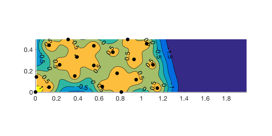
We model the (estimated) probability of hard braking using the negative logit function $-\log\frac{y}{1-y}$, which maps the outcome $y\in[0,1]$ from the simulator to the real line. This is not strictly needed but ensures that the Gaussian process is consistent with the type of output. We run an exploratory simulation with a budget of 20 points for Straddle, LSE and our algorithm. While the underlying function has some random noises due to the Monte Carlo simulation, we fix the seed to have the same point-wise responses from the simulator when different algorithms are tested. We select a threshold of 1.0 and again choose the origin as the initial seed. In Figure 6(a) we plot the contours for $\mu_{GP}(\mathbf{x})-1.96\sigma_{GP}(\mathbf{x})$. It can be seen that LSE and the Straddle heuristic both try to reduce the uncertainty by spreading out the sample points. Crucially, our algorithm places more samples together to compensate for the noise and reduce the variance (Figure 6(c)) in the promising region (Figure 6(b)) above $t=1.0$ . This allows the classifier to use the posterior GP to make a more confident prediction and identify the area of interest with high confidence (yellow region in Figure 6(a)).

References

- [1] A. Gotovos, N. Casati, G. Hitz, and A. Krause. Active learning for level set estimation. In International Joint Conference on Artificial Intelligence (IJCAI), pages 1344–1350, 2013.
- [2] C. E. Rasmussen and C. K. I. Williams. Gaussian Processes for Machine Learning. MIT Press, 2006.
- [3] B. Shahriari, K. Swersky, Z. Wang, R. P. Adams, and N. de Freitas. Taking the human out of the loop: A review of Bayesian optimization. 104(1):148 – 175, 2016.
- [4] H. J. Kushner. A new method of locating the maximum point of an arbitrary multipeak curve in the presence of noise. Journal of Basic Engineering, 86(1), 1964.
- [5] J. Mockus, V. Tiesis, and A. Zilinskas. The application of Bayesian methods for seeking the extremum. In L. C. W. Dixon and G. P. Szego, editors, Towards Global Optimization, volume 2. North-Holland Publishing Company, 1978.
- [6] N. Srinivas, A. Krause, S. M. Kakade, and M. Seeger. Gaussian process optimization in the bandit setting: No regret and experimental design. In International Conference on Machine Learning (ICML), pages 1015–1022, 2010.
- [7] B. Shahriari, Z. Wang, M. W. Hoffman, A. Bouchard-Cote, and N. de Freitas. An entropy search portfolio for Bayesian optimization. In Advances on Neural Information Processing Systems (NIPS), 2014.
- [8] R. M. Willet and R. D. Nowak. Minimax optimal level-set estimation. IEEE Transaction on Image Processing, 16(12):2965–2979, 2007.
- [9] A. Soni and J. Haupt. Level set estimation from compressive measurements using box constrained total variation regularization. In IEEE International Conference on Image Processing (ICIP), pages 2573–2576, 2012.
- [10] K. Krishnamurthy, W. U. Bajwa, and R. Willett. Level set estimation from projection measurements: Performance guarantees and fast computation. SIAM Journal on Imaging Sciences, 6(4):2047–2074, 2013.
- [11] A. Krause, A. Singh, and C. Guestrin. Near-optimal sensor placements in Gaussian processes: Theory, efficient algorithms and empirical studies. Journal of Machine Learning Research, 9:235–284, 2008.
- [12] L. Martino, J. Vicent, and G. Camps-Valls. Automatic emulator and optimized look-up table generation for radiative transfer models. In IEEE International Geoscience and Remote Sensing Symposium, pages 1457–1460, 2017.
- [13] D. Busby. Hierarchical adaptive experimental design for Gaussian process emulators. Reliability Engineering & System Safety, 94(7):1183 – 1193, 2009.
- [14] B. Bryan, R. C. Nichol, C. R. Genovese, J. Schneider, C. J. Miller, and L. Wasserman. Active learning for identifying function threshold boundaries. In Advances in neural information processing systems (NIPS), pages 163–170, 2005.
- [15] I. Bogunovic, J. Scarlett, A. Krause, and V. Cevher. Truncated variance reduction: A unified approach to Bayesian optimization and level-set estimation. In Advances in neural information processing systems (NIPS), pages 1507–1515, 2016.
- [16] J. Yang, Z. Wang, and J. Wu. Level set estimation with dynamic sparse sensing. In IEEE Global Conference on Signal and Information Processing (GlobalSIP), pages 487–491, 2014.
- [17] Y. Ma, R. Garnett, and J. Schneider. Active area search via Bayesian quadrature. In Artificial Intelligence and Statistics (AISTATS), pages 595–603, 2014.
- [18] Y. Ma, D. Sutherland, R. Garnett, and J. Schneider. Active pointillistic pattern search. In Artificial Intelligence and Statistics (AISTATS), pages 672 – 680, 2015.
- [19] J. Bect, D. Ginsbourger, L. Li, V. Picheny, and E. Vazquez. Sequential design of computer experiments for the estimation of a probability of failure. Statistics and Computing, 22(3):773–793, 2012.
- [20] C. Chevalier, J. Bect, D. Ginsbourger, E. Vazquez, V. Picheny, and Y. Richet. Fast parallel kriging-based stepwise uncertainty reduction with application to the identification of an excursion set. Technometrics, 56(4):455–465, 2014.
- [21] M. Treiber, A. Hennecke, and D. Helbing. Congested traffic states in empirical observations and microscopic simulations. 62(2):1805, 2000.
- [22] A. Kesting, M. Treiber, and D. Helbing. General lane-changing model MOBIL for car-following models. Transportation Research Record, 1999(1):86–94, 2007.
Appendix A: Technical Proofs
Lemma 1. The classification rule identified by Eqn. (3) minimizes the expected weighted misclassification error: