Relaxation Augmented Free Energy Perturbation

In recent years, Non-equilibrium physics has become a hot topic that encompasses many fields, including active matter Needleman and Dogic 2017, dissipative dynamics that break time-reversal sysmetry Dasbiswas et al. 2018, entropy production Onsager 1931; Gallavotti 2004, etc. Free energy calculations through non-equilibrium approaches is also one of them. Ever since the Jarzynski equality (JE) was first derived Jarzynski 1997, several ways to derive it have been published, including derivation via the Crooks theorem Crooks 2000 and via the Feynman–Kac theorem Hummer and Szabo 2001. Later on, different free energy estimators have also been proposed: for instance Adib’s clamp-and-release method rooted in microscopic reversibility Adib 2006, and the Non-equilibrium Candidate Monte Carlo (NCMC) Nilmeier et al. 2011 based on a path-wise detailed balance condition. Recently, it has been shown that the equilibrium free energy can be extracted from trajectories of the spontaneous thermal relaxation processes Ross et al. 2018. Inspired by this study and by the known interrelation between work and heat in thermodynamics, we investigate the role of heat released in a relaxation process, initiated by a single large perturbation, for free energy calculations.

Consider a system originally at the equilibrium end state $R$. If the system can be brought into the equilibrium end state $P$ by perturbing its Hamiltonian along a path, then JE states that the free energy difference between the two end states can be calculated through the average of the work done to the system over all paths Jarzynski 1997, i.e.

$\displaystyle e^{-\beta\Delta A}=\overline{e^{-\beta W}}\,\,\,,$

(1)

where $\Delta A$ is the Helmholtz free energy difference between states $P$ and $R$, and $\beta$ is the inverse temperature multiplied by the Boltzmann constant ($\beta=1/k_{B}T$). The work done to the system is denoted by $W$ and is defined as the accumulated energy change via varying the Hamiltonian along the path. The overline indicates the average is performed over all paths, as $W$ is path-dependent. Yet, the sampling of possible paths is not trivial: Depending on how the Hamiltonian is perturbed, different types of paths will be sampled, and different convergence behavior is thus expected. For instance, if the system is brought from state $R$ to $P$ instantaneously, i.e. the Hamiltonian is perturbed in one single step as in Fig. 1, the work done to the system is just the potential difference between the two end states, namely

$\displaystyle u(x)=U_{P}(x)-U_{R}(x)\,\,\,,$

(2)

where $u$ denotes the work (perturbation) done to the system, and $U_{P}(x)$ and $U_{R}(x)$ represent the potentials of state $P$ and $R$, respectively. In this scenario, it was shown that Jarzynski 1997 the path average is just the ensemble average over $R$, and the JE is equivalent to the single-step free energy perturbation (single-step FEP) Zwanzig 1954,

$\displaystyle\langle e^{-\beta\Delta A}\rangle=\langle e^{-\beta u}\rangle_{R}\,\,\,,$

(3)

where $\Delta A$ represents the Helmholtz free energy difference between two end states, and $\langle\cdots\rangle_{R}$ represents the NVT ensemble average over state $R$. Although Eq. 1 and Eq. 3 are both exact in theory, in practice they often fail to converge, because the sampling often misses the important rare events that have “negative work” (work smaller than the exact free energy $\Delta A_{\text{Exact}}$), see e.g. the green arrow depicted in Fig. 1. To overcome this insufficient sampling problem, calculations are usually conducted with a multi-step (slow switch) protocol Valleau and Card 1972, where the system’s Hamiltonian is perturbed gradually through several windows. Within each window, the free energy change can again be calculated using Eq. 1 or Eq. 3, and the free energy difference between state $P$ and state $R$ is given by the accumulated free energy change over all windows. Such operations are termed multi-step FEP Pohorille et al. 2010 or JE with a slow switch.

While the rare events (the high energy microstates that have work $u\leq\Delta A_{\text{Exact}}$) are not easy to sample, exploring the equilibrium microstates of $P$ is straightforward: after perturbing the system in one single step (blue line in Fig. 1), propagating the system with a heat bath coupled will result in a spontaneous relaxation that brings the system to the equilibrium of state $P$ Ross et al. 2018. Since both rare events and the relaxation explore the equilibrium of $P$, we would like to know whether the exact free energy can be calculated with the relaxation processes instead of the rare events. During the relaxation process, the extra potential energy is released as heat ($q$) into the heat bath, so the process violates the time-reversal symmetry (or microscopic reversibility Mahan 1975) Dasbiswas et al. 2018. Such a process is by its nature incompatible with the Crooks theorem as well as the Adib’s nonequilibrium method because both of them are rooted in microscopic reversibility. An alternative derivation outside of those frameworks is thus needed to include the heat released from the relaxation process.

We begin with a harmonic oscillator model as depicted in Fig. 1, at the low temperature limit ($\beta\to\infty$). For simplicity, the potentials of the two end states $R$ and $P$ are chosen as $U_{R}(x)=\frac{1}{2}kx^{2}$ and $U_{P}(x)=\frac{1}{2}k(x-d)^{2}+U_{0}$, respectively. At $\beta\to\infty$, the probability distribution $P_{R}(x)$ can be approximated by the Dirac delta function as,

$\displaystyle\lim_{\beta\to\infty}P_{R}(x)=\lim_{\beta\to\infty}\frac{1}{\sqrt{2\pi/k\beta}}\exp[-(\frac{x}{\sqrt{2/k\beta}})^{2}]=\delta(x)\,.$

(4)

In the context of sampling, Eq. 4 states that the sampling is trapped at one single configuration ($x=0$), and the associated work is given by $u=U_{P}(0)-U_{R}(0)=U_{0}+kd^{2}/2$. Following the conventional definition Nilmeier et al. 2011, the heat $q$ released in the relaxation process reads,

$\displaystyle q(x,x^{\prime})=U_{P}(x^{\prime})-U_{P}(x)\,\,\,,$

(5)

where $x$ and $x^{\prime}$ are configurations before and after the relaxation, respectively. Similarly, the end point of the relaxation can only be at $x^{\prime}=d$, with the heat $q=U_{P}(d)-U_{P}(0)=-kd^{2}/2$ released. Since the analytic exact free energy is given by $\Delta A_{\text{Exact}}=U_{0}$, it is not difficult to see that $\Delta A_{\text{Exact}}=u+q$, leading to a working equation:

$\displaystyle e^{-\beta\Delta A_{\text{Exact}}}=\overline{e^{-\beta(u+q)}}=\langle e^{-\beta(u+q)}\rangle_{R}\quad,$

(6)

which appears as a natural extension of Eq. 1 and Eq. 3, with an extra term $q$ in the average. Although this equation only holds at the low temperature limit, it takes into account the heat released in a relaxation path, and hence will be termed “relaxation augmented free energy perturbation” (RAFEP). Results of applying Eq. 6 to harmonic oscillators with different deviation $d$ at 0.1 K are depicted in Fig. 2(a). Compared to JE/FEP with a single step perturbation (via Eq. 3), RAFEP (via Eq. 6) agrees well with the exact solution $\Delta A_{\text{Exact}}$ at 10 kcal/mol, c.f. the blue and orange dots to the black line. This confirms that microscopically the heat released during relaxation can contribute to the free energy difference between two end states.

Moreover, calculations with JE/FEP and RAFEP are both performed using $10^{9}$ Monte Carlo (MC) steps with a step size 0.1 Å. The former spends it all on sampling the equilibrium state $R$, but still fails to sample the important rare events. The latter first collects 5000 microstates from a simulation of $5\times 10^{4}$ steps, and then relaxes each collected microstates with a $2\times 10^{4}$ step-long simulation. Thus the good performance of RAFEP can only be attributed to introducing the relaxation process ($q$) into the free energy calculation.

What happens at higher temperature? There the thermal fluctuation causes the system to populate numerous configurations, leading to paths with various values of $u$ and $q$. While the path average remains the same as in Eq. 6, the ensemble average shown in Eq. 6 does not yet account for the thermal fluctuation on state $P$, which would require an extra ensemble average over state $P$. That is, the two averages are related via

$\displaystyle\overline{e^{-\beta(u+q)}}=\langle\langle e^{-\beta(u+q)}\rangle_{R}\rangle_{P}\quad.$

(7)

The double layer ensemble average in Eq. 7 means that from every sampled microstate of $R$, multiple relaxation runs should be performed to sample different microstates of $P$. Numerical evaluations of the terms in Eq. 7 are depicted in Fig. 3(a). Shown there are the quantities $-k_{B}T\ln\overline{e^{-\beta(u+q)}}$ and $-k_{B}T\ln\langle\langle e^{-\beta(u+q)}\rangle_{R}\rangle_{P}$, using totally $10^{10}$ relaxation steps. The path average distributes these steps into relaxing $5\times 10^{5}$ microstates of $R$ (relaxation length $2\times 10^{4}$ as before), while the ensemble average repeats relaxing the same 5000 microstates 100 times each. Clearly, when the temperature is higher, the ensemble average will suffer from a larger fluctuation, cf. the red dots shown in Fig. 3(a). Nevertheless, the two averages agree well for $T<160$ K.

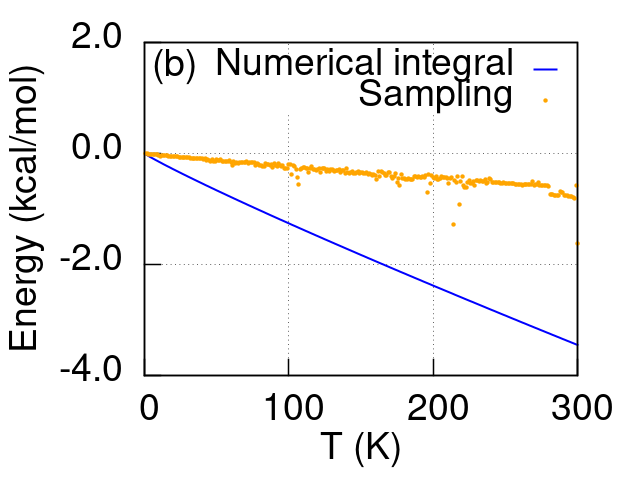
Interestingly, both averages deviate from $\Delta A_{\text{Exact}}$ (black line) as temperature $T$ increases, and the deviation is even larger if one evaluates $-k_{B}T\ln\langle\langle e^{-\beta(u+q)}\rangle_{R}\rangle_{P}$ by numerical integration (boundary used: -1000 Å to 1000 Å), as shown by the blue line. Perhaps this is not so surprising. Following the definition of work and heat (Eq. 2 and Eq. 5), the ensemble average can be arranged to

$\displaystyle\langle\langle e^{-\beta(u+q)}\rangle_{R}\rangle_{P}=\langle e^{-\beta U_{P}(x^{\prime})}\rangle_{P}\langle e^{+\beta U_{R}(x)}\rangle_{R}\quad.$

(8)

Evaluation of $\langle e^{-\beta U_{P}(x^{\prime})}\rangle_{P}$ via integration and via sampling give an identical value, but evaluation of $\langle e^{+\beta U_{R}(x)}\rangle_{R}$ by the two methods does not, cf. the orange dots and blue line in Fig. 3(b). When expressing this term as an integral,

$\displaystyle\langle e^{+\beta U_{R}}\rangle_{R}=\int e^{+\beta U_{R}(x)}P_{R}(x)dx\quad,$

(9)

where $P_{R}(x)$ denotes the probability distribution of state $R$, one sees the problem immediately. For an NVT ensemble, $P_{R}(x)$ is normally taken as the Boltzmann distribution $e^{-\beta U_{R}(x)}/Z_{R}$ with $Z_{R}$ representing the associated partition function. This results in a diverging integral $\int 1\,dx/Z_{R}$, if no extra integration boundary is imposed. As we are using an integration boundary ($-1000$ Å to $1000$ Å), the blue line depicted in panels (a) and (b) simply reflects this size. In contrast, the MC sampling always results in a particle position trapped within $\pm$9 Å from the potential minimum. This kind of trapped finite sampling is traditionally considered to be the problem for evaluating integrals via sampling, e.g. Eq.3 can be derived via integration formalism Chipot and Pohorille 2007 but is problematic when evaluated via sampling. Various enhanced sampling methods have been developed to overcome this problem Sugita and Okamoto 1999; Limongelli et al. 2013. However, as the sampling results (orange and red dots) depicted in Fig. 3(a) follow $\Delta A_{\text{Exact}}$ better than the numerical integration (blue line) does, it may be worth formulating the problem differently. Namely, by admitting that the ergodicity is violated in a finite sampling, we can describe a finite sampling’s behavior with an approximated $P_{R}(x)$ that reads,

$\displaystyle P_{R}(x)\approx\frac{e^{-\beta U_{R}(x)}}{Z_{R}}\cdot\theta(U_{R}^{*}-U_{R}(x))\quad,$

(10)

where $\theta(U_{R}^{*}-U_{R}(x))$ denotes a Heaviside step function that caps the population in energy space, based on the maximum energy $U_{R}^{*}$ encountered during the sampling. We note that Eq. 10 does not change the actual sampling but rather the formalism of how a finite sampling relates to the associated partition function, i.e. inserting Eq. 10 into Eq. 9 results in

$\displaystyle\langle e^{+\beta U_{R}}\rangle_{R}$

$\displaystyle\approx$

$\displaystyle\frac{\int\theta(U_{R}^{*}-U_{R}(x))dx}{Z_{R}}=\frac{V_{R}}{Z_{R}}\quad,$

(11)

with $V_{R}=\int\theta(U_{R}^{*}-U_{R}(x))dx$ defining the volume of configuration space that is actually accessed during a finite sampling of $R$. Similarly for state $P$,

$\displaystyle\langle e^{+\beta U_{P}}\rangle_{P}$

$\displaystyle\approx$

$\displaystyle\frac{\int\theta(U_{P}^{*}-U_{P}(x))dx}{Z_{P}}=\frac{V_{P}}{Z_{P}}\quad,$

(12)

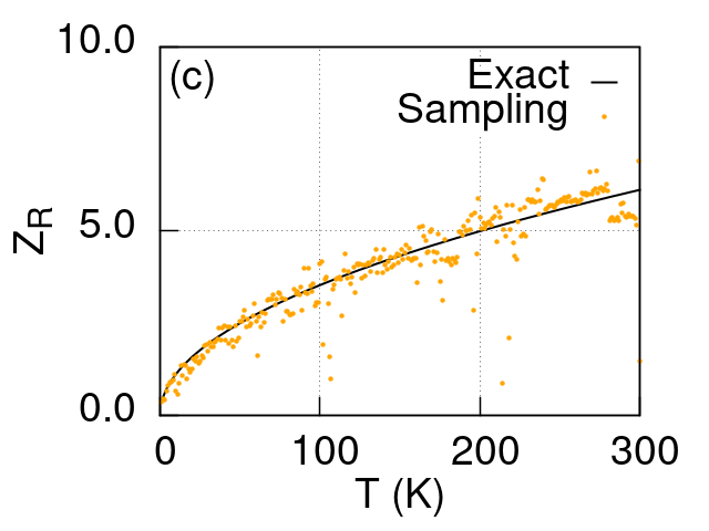
where the volume of accessed configuration space is denoted by $V_{P}=\int\theta(U_{P}^{*}-U_{P}(x))dx$, with $U_{P}^{*}$ denoting the maximum energy sampled for state $P$. Notably, adopting this approximation means that one can estimate the partition function directly from a finite sampling. Fig. 3(c) shows how $Z_{R}$ can be sampled by using Eq. 11, where the volume $V_{R}$ is here taken from the distance between maximum and minimum $x$ of a trajectory. Following Eq. 11 and Eq. 12, the RAFEP estimator for arbitrary potential and arbitrary temperature reads,

$\displaystyle e^{-\beta\Delta A_{\text{Exact}}}\approx\frac{\langle e^{+\beta U_{R}}\rangle_{R}}{\langle e^{+\beta U_{P}}\rangle_{P}}\cdot\frac{V_{P}}{V_{R}}\quad,$

(13)

which can be combined with Eq. 7 and Eq. 8 to give,

$\displaystyle e^{-\beta\Delta A_{\text{Exact}}}\approx\frac{\overline{e^{-\beta(u+q)}}}{\langle e^{-\beta U_{P}}\rangle_{P}\langle e^{+\beta U_{P}}\rangle_{P}}\cdot\frac{V_{P}}{V_{R}}\quad.$

(14)

Thus, the above two equations are the estimator in two different forms. Eq. 13 combines the samples from two end states for $\Delta A_{\text{Exact}}$, and is functionally similar to the Bennett acceptance ratio (BAR) Bennett 1976. Eq. 14 states how the calculation can be performed from an equilibrium end state $R$, going through paths including an instantaneous perturbation and a subsequent relaxation to arrive at the equilibrium of state $P$.

Results of RAFEP via Eq. 13 for displaced harmonic oscillators at 300 K are depicted in Fig. 2(b). Calculations are conducted by combining 5000 samples collected over $5\times 10^{4}$ MC steps for state $R$ and for state $P$, according to Eq. 13. For comparison, JE/FEP calculations via Eq. 3 are also performed using the same amount of sampling, and the associated results are further combined through BAR Bennett 1976. Indeed, BAR recovers $\Delta A_{\text{Exact}}$ (10 kcal/mol, black line) when $d$ is small, but it still fails when $d\geq 17$ Å. In contrast, RAFEP via Eq. 13 outperforms BAR in this specific case. Although not depicted here, RAFEP calculations via Eq. 14 using $10^{9}$ steps are also performed, and the same results as those shown in Fig. 2(b) are found. Either way, the good performance suggests that RAFEP grasps relevant physics, even without sampling the rare events.

Next we apply RAFEP to calculate the free energy change upon inserting one argon (Ar) atom into $N-1$ Ar atoms in a box of size 1000 Å³ with periodic boundary conditions. By varying $N$, particle densities from gas to solid phase can be explored. The temperature is set to 85 K, while the Lennard-Jones parameters are taken from literature Frenkel and Smit 2001: $\epsilon=0.238$ kcal/mol and $\sigma=3.405$ Å. The validity of the finite sampling approximation (Eq. 11 and Eq. 12) is easily justified by looking at the trajectory histogram of two Ar atoms placed in a one-dimensional box, see Fig. 4(a) where the unpopulated white stripe echoes the violation of ergodicity in a finite sampling ($2\times 10^{6}$ step MC simulation for this example).

Results of the free energy change upon inserting one Ar atom are shown in Fig. 4(b). As no analytic solution is available, the numerically exact reference is taken from multi-step FEP calculations combined with BAR (labeled as mFEP-BAR). For each $N$, the sampling is performed using totally $2\times 10^{9}$ MC steps, shared between two mFEP calculations (initiated from $R$ and $P$) with 100 windows each, where $10^{7}$ steps are employed within each window. Note that BAR Bennett 1976 is mandatory to combine the samples from the two mFEP calculations, as their results differ by up to 7.6 $k_{B}T$. When $N\geq 24$, the particle density is comparable with solid Ar, and inserting one Ar atom would cause a significant reorganization of other Ar’s positions within the box. This results in a zigzag shape for $\Delta A$, which is also observed in the result of Widom insertion Widom 1963 (blue curve). Widom insertion can be viewed as an improved version of Eq. 3, where the single uncoupled Ar can be separated from the other $N-1$ atoms for brute-force enhanced sampling: here $2\times 10^{7}$ steps are used to sample the $N-1$ atoms, and each sampled configuration is further subjected to 100 MC samples of the single Ar. In total, the Windom calculation also utilizes $2\times 10^{9}$ MC steps, but the method does not reproduce $\Delta A_{\text{Exact}}$ at high particle density, owing to missing relevant rare events where the $N-1$ Ar atoms should reorganize to accommodate the inserted atom. In contrast, RAFEP via Eq. 13 (orange curve) follows closely the numerical reference, even when $N>24$. This good performance again confirms that RAFEP indeed grasps the relevant physics. Notably, for RAFEP the ensemble averages are calculated with $10^{7}$ samples for each end state, which is repeated 10 times to account for statistical fluctuations, while $V_{R}$ and $V_{P}$ are now calculated via nested sampling Skilling 2004; Bernstein et al. 2016; Baldock et al. 2017; Pártay et al. 2010, each with operations equivalent to $0.288\times 10^{9}$ MC steps. Hence, each RAFEP calculation employs $0.776\times 10^{9}$ MC steps – less than half needed for mFEP-BAR.

We have presented a new estimator that is motivated from trying to incorporate the heat released during the relaxation process following a single step perturbation, into free energy calculations. To avoid the limitation of employing microscopic reversibility, a new derivation based on observing the finite sampling behavior is presented. This results in the new estimator RAFEP, which explicitly admits the violation of ergodicity in a finite sampling and utilizes a volume term to account for this feature. RAFEP is then applied to displaced harmonic oscillators and particle insertion with Ar atoms. In both examples, it proves to be a valid estimator and is free from the need of sampling rare events, demonstrating that RAFEP provides an alternative and conceptually new view on the underlying physics. Although it is outside the scope of the current paper, scaling up RAFEP calculations for biological systems may be of great interest Cournia et al. 2017. Crucially the performance of RAFEP depends on how fast the volume terms can be calculated. For lower dimensions, these can be determined effortlessly from a trajectory histogram. This approach soon becomes impossible as its memory usage growths exponentially as the dimensionality increases. Yet the hope remains in further advancing the computational methods, such as nested sampling Skilling 2004; Pártay et al. 2010, population annealing Christiansen et al. 2019, and non-equilibrium importance sampling Rotskoff and Vanden-Eijnden 2019.

References

- Needleman and Dogic (2017) D. Needleman and Z. Dogic, Nat. Rev. Mater. 2, 17048 (2017).
- Dasbiswas et al. (2018) K. Dasbiswas, K. K. Mandadapu, and S. Vaikuntanathan, Proc. Natl. Acad. Sci. U.S.A. 115, E9031 (2018).
- Onsager (1931) L. Onsager, Phys. Rev. 37, 405 (1931).
- Gallavotti (2004) G. Gallavotti, Chaos 14, 680 (2004).
- Jarzynski (1997) C. Jarzynski, Phys. Rev. Lett. 78, 2690 (1997).
- Crooks (2000) G. E. Crooks, Phys. Rev. E 61, 2361 (2000).
- Hummer and Szabo (2001) G. Hummer and A. Szabo, Proc. Natl. Acad. Sci. U.S.A. 98, 3658 (2001).
- Adib (2006) A. B. Adib, J. Chem. Phys. 124, 144111 (2006).
- Nilmeier et al. (2011) J. P. Nilmeier, G. E. Crooks, D. D. L. Minh, and J. D. Chodera, Proc. Natl. Acad. Sci. U.S.A. 108, E1009 (2011).
- Ross et al. (2018) D. Ross, E. A. Strychalski, C. Jarzynski, and S. M. Stavis, Nat. Phys. 14, 842 (2018).
- Zwanzig (1954) R. W. Zwanzig, J. Chem. Phys. 22, 1420 (1954).
- Valleau and Card (1972) J. P. Valleau and D. N. Card, J. Chem. Phys. 57, 5457 (1972).
- Pohorille et al. (2010) A. Pohorille, C. Jarzynski, and C. Chipot, J. Phys. Chem. B 114, 10235 (2010).
- Mahan (1975) B. H. Mahan, J. Chem. Educ. 52, 299 (1975).
- Bennett (1976) C. H. Bennett, J. Comput. Phys. 22, 245 (1976).
- Chipot and Pohorille (2007) C. Chipot and A. Pohorille, Free Energy Calculations: Theory and Applications in Chemistry and Biology (Springer, 2007).
- Sugita and Okamoto (1999) Y. Sugita and Y. Okamoto, Chem. Phys. Lett. 314, 141 (1999).
- Limongelli et al. (2013) V. Limongelli, M. Bonomi, and M. Parrinello, Proc. Natl. Acad. Sci. U.S.A. 110, 6358 (2013).
- Frenkel and Smit (2001) D. Frenkel and B. Smit, Understanding Molecular Simulation (Academic Press, Inc., Orlando, FL, USA, 2001), 2nd ed., ISBN 0122673514.
- Widom (1963) B. Widom, J. Chem. Phys. 39, 2808 (1963).
- Skilling (2004) J. Skilling, AIP Conf. Proc. 735, 395 (2004).
- Bernstein et al. (2016) N. Bernstein, R. J. N. Baldock, L. B. Pártay, J. R. Kermode, T. D. Daff, A. P. Bartók, and G. Csányi, pymatnest, https://github.com/libAtoms/pymatnest (2016).
- Baldock et al. (2017) R. Baldock, N. Bernstein, K. M. Salerno, L. B. Pártay, and G. Csányi, Phys. Rev. E. 96, 043311 (2017).
- Pártay et al. (2010) L. B. Pártay, A. P. Bartók, and G. Csányi, J. Phys. Chem. B 114, 10502 (2010).
- Cournia et al. (2017) Z. Cournia, B. Allen, and W. Sherman, J. Chem. Inf. Model. 57, 2911 (2017).
- Christiansen et al. (2019) H. Christiansen, M. Weigel, and W. Janke, Phys. Rev. Lett. 122, 060602 (2019).
- Rotskoff and Vanden-Eijnden (2019) G. M. Rotskoff and E. Vanden-Eijnden, Phys. Rev. Lett. 122, 150602 (2019).
Acknowledgements
Y-C.C. thanks Prof. Jarzynski for helpful discussions, the Royal Society for funding (NF171278), and the iSolution at the University of Southampton for computing time on the Iridis5 cluster. L.B.P. acknowledges support from the Royal Society through a Dorothy Hodgkin Research Fellowship.