Kinetic Methods for Inverse Problems
Abstract
The Ensemble Kalman Filter method can be used as an iterative numerical scheme for parameter identification or nonlinear filtering problems. We study the limit of infinitely large ensemble size and derive the corresponding mean-field limit of the ensemble method. The solution of the inverse problem is provided by the expected value of the distribution of the ensembles and the kinetic equation allows, in simple cases, to analyze stability of these solutions. Further, we present a slight but stable modification of the method which leads to a Fokker-Planck-type kinetic equation. The kinetic methods proposed here are able to solve the problem with a reduced computational complexity in the limit of a large ensemble size. We illustrate the properties and the ability of the kinetic model to provide solution to inverse problems by using examples from the literature.
Mathematics Subject Classification (2010)
35Q84, 65N21, 93E11, 65N75
Keywords
Kinetic Partial Differential Equations, Nonlinear Filtering Methods, Inverse Problems
1 Introduction
We are concerned with the following abstract inverse problem or parameter identification problem
| (1) |
where is the (possible nonlinear) forward operator between finite dimensional Hilbert spaces and , with , is the control, is the observation and is observational noise. Given noisy measurements or observations and the known mathematical model , we are interested in finding the corresponding control . Typically, the observational noise is not explicitly known but only information on its distribution is available. Inverse problems, in particular in view of a possible ill-posedness, have been discussed in vast amount of literature and we refer to [20] for an introduction and further references. In the following we will investigate a particular numerical method for solving problem (1), namely, the Ensemble Kalman Filter (EnKF). While this method has already been introduced more than ten years ago [22], recent theoretical progress [46] is the starting point of this work.
As in [46] we aim to solve the inverse problem by minimizing the least squares functional
| (2) |
where normalizes the so-called model-data misfit. This is defined as the covariance of the noise . Note that there is no regularization of the control in the minimization problem of (2). See e.g. [5, 25, 27, 33] for examples of Tikhonov and other regularization technique.
We briefly recall a Bayesian inversion formulation for problem (1). Following [15, 48] a solution to the inverse problem is obtained by treating the unknown control , the data and the noise as random variables. Then, the conditional probability measure of the control given the observation , called posterior measure, is computed via Bayes Theorem. Typically, there is an interest in moments of the posterior, e.g. choosing the point of maximal probability (MAP estimator). For further details concerning Bayesian inversion, e.g. the modeling of the unknown prior distributions and other choices of estimators, see [4, 9, 15, 21] and references therein.
Before finally stating the aim of this work, we briefly recall some references on the EnKF method without aiming to give a complete list. Iterative filtering methods have also been successfully applied to inverse problems since many years. A particular successful method has been originally proposed in [32] to estimate state variables, parameters, etc. of stochastic dynamical systems. This method has been extended to the EnKF in [22]. The EnKF sequentially updates each member of an ensemble of random elements in the space by means of the Kalman update formula, using the knowledge of the model and of given observational data . It is important to note that no information on the derivative of is required. The EnKF provides satisfactory results even when used with a small number of ensembles, as proved by the accuracy analysis in [40]. Some examples in mathematical literature of the application of the filtering method to inverse problems are given in the incomplete list [1, 6, 7, 29, 30, 46, 47]. In particular, we refer to the following books [23, 42]. Our starting point is [46] where the continuous time limit of the EnKF has been studied as a regularization technique for minimization of the least squares functional (2) with a finite ensemble size. Recently, further study has been conducted in this direction [13, 35]. We also note that the EnKF can also formally be derived within the Bayesian framework [21, 31, 34, 36, 38].
In the cited references the ensemble size was fixed and, due to the possible associated high computational cost, limited to a small number of ensembles. The analysis of the method for a large ensemble size limit has been investigated in [16, 17, 21, 37]. However, to the best of our knowledge, an evolution equation for the probability distribution of the unknown control has not been derived. We aim to provide a continuous representation of the EnKF method that also holds in the limit of infinitely many ensembles. We do believe that the derivation of the kinetic equation leads to insight to the method that might not be easy to obtain otherwise. The main advantage of the derivation of a mean-field equation is twofold. First, it formally allows to deal with the case of infinitely many ensembles and in this regime numerical simulations show a better reconstruction of an estimator of the unknown control than considering small ensemble sizes. Second, it allows to study stability, at least in the simple case of a one-dimensional control, and it suggests a modification of the method which results in improved stability of the corresponding Fokker-Planck equation.
We proceed as follows: We start from the continuous time limit formulation of the EnKF derived in [46] and interpret it as an interacting particle system. Then, we study the mean-field limit for large ensemble sizes. From a mathematical point of view, this technique has been widely used to reduce the computational complexity and to analyze interacting particle models, e.g. in socio-economic dynamics or gas dynamics [11, 12, 14, 26, 28, 44, 49, 50]. The kinetic equation evolves in time the probability distribution of the control and the solution to the inverse problem is shown to be the mean of this distribution. We analyze linear stability of the EnKF. Further, we present suitable modifications of the method based on the kinetic formulation in order to improve the stability pattern. The kinetic model guarantees a computational gain in the numerical simulations using a Monte Carlo approach similar to [2, 8, 24, 39, 41, 43, 44].
2 From the Ensemble Kalman Filter to the gradient descent equation
The Ensemble Kalman Filter (EnKF) has been introduced [22] as a discrete time method to estimate state variables, parameters, etc. of stochastic dynamical systems. The estimations are based on system dynamics and measurement data that are possibly perturbed by known noise. The EnKF is a generalization and improved version of the classical Kalman Filter method [32]. In the following, we briefly review the definition of the EnKF which is based on a sequential update of an ensemble of states and parameters. Then we recover the continuous time limit equation derived in the recent work [46]. This will be the starting point to introduce and compute in the next sections a mean-field limit for infinitely many ensembles. The arising kinetic partial differential equation allows subsequent analysis on the nature of the method.
As in [46] we consider a control , a given state coupled by the system dynamic as stated by equation (1). The problem is to identify the unknown control given possibly perturbed measurements of the state Hence, the observation of the system dynamic is perturbed by noise . The noise is assumed independent on the control and normally distributed with zero mean and known covariance matrix , i.e. . We consider a number of ensembles (realizations of the control) combined in . The EnKF is originally posed as a discrete iteration on The iteration index is denoted by and the collection of the ensembles by , and . According to [46], the EnKF iterates each component of at iteration as
| (3) | ||||
for each . Here, each observation or measurement has been perturbed by , and is a parameter. As in [46] two cases for the covariance will be discussed: corresponding to a problem where the measurement data is unperturbed and corresponding to the case where are realizations of the noise
Note that the update (3) of the ensembles requires the knowledge of the operators and which are the covariance matrices depending on the ensemble set at iteration and on , i.e. the image of at iteration . More precisely,
| (4) | ||||
where we define by and the mean of and , namely
In recent years, the EnKF was also studied as technique to solve classical and Bayesian inverse problems. For instance see the works [30] and [21], respectively, and the references therein. Here, we keep the attention on this type of application. The analysis of the method is proved to have a comparable accuracy with traditional least-squares approaches to inverse problems [30]. Moreover, it is known that the method provides an estimate of the unknown control which lies in the subspace spanned by the initial ensemble set [30]. We will see in this section that this property is still true at the continuous time level [46]. Concerning Bayesian inverse problems, instead, the method is proved to approximate specific Bayes linear estimators but it is able to provide only an approximation of the posterior measure by a (possibly weighted) sum of Dirac masses. For a detailed discussion we refer to [3, 21, 38].
As showed in [46], it is straightforward to compute the continuous time limit equation of the update (3) in the general case of a nonlinear model , even if the asymptotic analysis was performed in the easier linear setting. Consider the parameter as an artificial time step for the iteration in (3), i.e. we take where is the maximum number of iterations. Assume then for . Scaling by and computing the limit , the continuous time limit equation of (3) reads
| (5) |
for , initial condition and are Brownian motions. Using the definition of the operator , see (4), system (5) can be restated as
| (6) |
for , where and is the inner-product on . From (6) it is easy to observe that the invariant subspace property holds also at the continuous time level in the case since the vector field is in the linear span of the ensemble itself.
In [46] the asymptotic behavior of the continuous time equation is analyzed in the linear setting with so that (5) is written as gradient descent equation. In fact, let us consider the case of linear, i.e. . Then the computation of the operator is Further, note that the least squares functional (2) yields
| (7) |
Therefore, equation (5) is stated in terms of the gradient of as
| (8) |
for . Equation (8) describes a preconditioned gradient descent equation for each ensemble. In fact, is positive semi-definite and hence
Observe that, although the forward operator is assumed to be linear, the gradient flow is nonlinear. For further details and properties of the gradient descent equation (8) we refer to [46]. In particular, here we recall the important result on the velocity of the collapse of the ensembles towards their mean in the large time limit.
Lemma 2.1 (Theorem 3 in [46]).
Let be the initial set of ensembles. Then the matrix whose entries are
converges to for and indeed .
The previous Lemma also states that the collapse slows down linearly as the ensemble size increases. Later, this property is also obtained in the mean-field limit for a large ensemble size.
3 Mean-field limit of the Ensemble Kalman Filter
Typically, the EnKF method is applied for a fixed and finite ensemble size. In fact, it is clear from (3) and (6) that the computational and memory cost of the method increases with the number of the ensembles. The analysis of the method was also studied in the large ensemble limit, see e.g. [21, 34, 37, 38]. However, to the best of our knowledge, the derivation of a kinetic equation that holds in the limit of a large number of ensembles has not yet been proposed. In this section, we derive the corresponding mean-field limit of the continuous time equation focusing on the case of a linear model and with as in [46].
We follow the classical formal derivation to formulate a mean-field equation of a particle system, see [11, 26, 44, 49]. Let us denote by
| (9) |
the compactly supported on probability density of at time and introduce the first moment and the second moment of at time , respectively, as
| (10) |
Since , the corresponding discrete measure on the ensemble set is therefore given by the empirical measure
| (11) |
where is the component of the -th ensemble. Let us define the operator
with the corresponding entry
where denotes the component of the mean of the ensembles. This formulation allows for a mean-field limit as
and therefore can be written in terms of the moments (10) of the empirical measure only as
| (12) |
Let us denote a sufficiently smooth test function. We compute
which finally leads to the following strong form of the mean-field kinetic equation corresponding to the gradient descent equation (8):
| (13) |
Equation (13) provides a closed formula for the evolution in time of the distribution of the unknown control when the observations and the linear model are given and when endowed with an initial guess for the unknown control.
3.1 Moment equations and linear stability analysis
As discussed in Section 2, the EnKF computes a solution to the inverse problem as mean of the ensembles in the large time behavior. Since the kinetic equation (13) formally holds in the limit of a large number of ensembles, here we analyze approximations to the solution of the inverse problem provided by the first moment of the kinetic distribution, see (10).
Due to definition (10), multiplying (13) by , integrating over and integrating by parts the second term, we get the following evolution equation for the first moment:
In particular, since we are assuming the simple setting of a linear model , using (7), we can explicitly compute the integral and obtain
| (14) |
Multiplying (13) by and integrating over we obtain the following evolution equation for the second moment:
| (15) |
Remark 3.1.
As in Bayesian approach to inverse problems, also equation (13) poses the problem of selecting a solution out of which only provides a distribution for the unknown control . As pointed out at the beginning of this subsection, since the kinetic equation is derived via mean-field limit we choose, accordingly to the solution provided by the EnKF, the expected value as an estimator of the unknown parameter . Observe that a steady-state of equation (14) is given by
corresponding to a control that minimizes the least squares functional . In the case of a linear model , the above condition can be also stated as Neither nor need to be unique.
Equation (14) for the first moment and (15) for the second moment give rise to a coupled system of ordinary differential equations. In the following, we employ a stability analysis for these equations in the simple case of a one-dimensional control in order to analyze the stability of the estimator .
First, we observe that in the case of a scalar control the system of the moment equations reduces to
| (16) | ||||
with and . The nullclines of the system of ODEs (16) are given by
The equilibrium or fixed points of (16) are the intersections of the nullclines and therefore we have the following three sets of points:
i.e. all the fixed points are on the parabola in the phase plane . Given the Jacobian of the ODE system (16)
| (17) |
it follows that has eigenvalues . Clearly, the same holds for and , since they are points of the type . Therefore all the fixed points are non-hyperbolic and the stability must be analyzed directly. More precisely, since , the fixed points are Bogdanov-Takens-type equilibria and hence unstable as we indeed show in the following analysis.
The vector field of the system (16) can be easily analyzed on nullclines and on the - and -axis of the phase plane. For the sake of simplicity, let us assume that . The analysis is equivalent in the opposite case. Let so that for all . We have that
and therefore is decreasing in time on the nullcline which in turn means that is an attractor only if . Let now , for some . Then we have and
Thus, since is the only acceptable initial condition in order to guarantee that , the trajectories are moving on the right side of the phase plane on the nullcline . Obviously, each trajectory is still in time on the nullcline since . The nullclines and the complete vector field for the case is shown in the left panel of Figure 1. We immediately observe that the behavior around the equilibrium point is unstable as showed also in the right panel of Figure 1.
The previous considerations can be also derived by looking at the solutions of (16). Assuming that the initial conditions are such that , we get then the following pairs of analytical solutions:
with constants uniquely prescribed by the initial conditions. In particular, the first set of solutions is found by assuming that and solving the following Riccati’s equation with constant coefficients
In this case, letting , the constant is given by which is positive when and negative otherwise. In this latter case we also observe that there exists a time in which the trajectory has a vertical asymptote. For the above discussion we know that is also decreasing. It is also simple to observe that in the second pair of solutions can blow up driving away from the equilibrium.
Remark 3.2.
We observe that the linear stability analysis provided in this section is applied to system (16) without including restrictions on which must be non-negative. Under this constraint, the region is not admissible and the unstable equilibrium lies on the boundary of this region.
4 Extension of the mean-field EnKF method
The analysis of Section 3.1 shows that, at least in a one-dimensional setting, the system of moment equations (16) could lead to unconditionally unstable equilibria. This is due to the possible decay of the energy which drives the expected value far from the equilibrium value. In the general case of a -dimensional control , the situation may be even more complex.
The instability of fixed points of (16) can be related to the loss of an term in the derivation of the continuous time limit equation (5). In fact, instability could occur also for (8) but it is possible to show that the discrete equation (3) has stable equilibria.
Next, we stabilize the system of the moment equations (16) by introducing additional uncertainty to the microscopic interactions. This leads to a diffusive term in the kinetic equation avoiding the decay of kinetic energy and the appearance of unstable equilibria. First, we write binary microscopic interactions corresponding to the mean-field kinetic equation (13). Then, we introduce noise in these interactions and we derive a Fokker-Planck-type equation. Finally, we study the stability of the resulting moment system.
Let again be the probability density of the control at time as defined in (9). Let and be the first and the second moment of , respectively, as given in (10). We introduce the microscopic interaction rules:
| (18) | ||||
where is the post-interaction value of the ensemble member, is its pre-interaction value and is a random variable with given distribution having zero mean and covariance matrix . Instead, is an arbitrary function of . For we observe a similar structure as in equation (5). The quantity describes the strength of the interactions and it is a scattering rate.
Remark 4.1.
Observe that (18) is in fact the microscopic interaction corresponding to the mean-field equation (13), that is in the case of a linear model
| (19) |
with an additional term representing the uncertainty in the interaction. The interaction (19) has a probabilistic interpretation [2] provided
where is the spectral radius.
The probability density satisfies the following (linear) Boltzmann equation in weak form
| (20) |
where is a test function and where the operator denotes the mean with respect to the distribution , i.e. Consider the time asymptotic scaling by setting
| (21) |
and allow . This corresponds to large interaction frequencies and small interaction strengths, a situation similar to the so-called grazing collision limit [18, 19, 45, 51]. We denote the scaled quantities again by and respectively. A second-order Taylor expansion yields the corresponding formal Fokker-Planck equation:
with , and where is the Hessian matrix and Substituting this expression in equation (20) and using definition (18) of the microscopic interactions, we obtain
where is the matrix trace and is the remaining term. One can easily prove that vanishes in the asymptotic scaling (21). In order to show this, it is sufficient the fact that is an enough smooth function and thus each second partial derivative is Lipschitz continuous so that such that
for all .
For constant or depending on moments of the kinetic distribution , the grazing limit in strong form is then obtained as
| (22) |
where we used the basic fact
Some remarks are in order. As expected, the Fokker-Planck-type equation (22) is consistent with the kinetic equation (13) in the limit of vanishing covariance . The introduction of the uncertainty in (18) allows for a different interpretation of the data perturbation in (3) and (6) within the kinetic model.
4.1 Moment equations and linear stability analysis
In the setting of [46] we have and, for identity matrix, a straightforward computation leads to the following moment equations based on the Fokker-Planck equation (22).
| (23) | ||||
where and are defined as before and where we have
Comparing equation (23) and (14), we observe that they are equivalent. This implies that the equation for is still providing a solution according to Remark 3.1. Instead, the equation of the second moment has an additional term that stabilize the equilibria of (23).
We analyze linear stability of (23) in the case of a one-dimensional control. In this particular case the moment equations are
| (24) | ||||
with , and where now represents the variance of the univariate noise . Following the same analysis performed in Section 3.1, we compute the nullclines of the ODE system (24) and they are given by
We are interested in the behavior around the equilibrium with which is obtained as intersection of the first and the third nullcline:
Observe that this equilibrium point is in fact the equilibrium point given in Section 3.1 when . For simplicity, in the following we consider . Similar considerations can be done in the other cases. Letting so that for all , we have
where the right-hand side represents a parabola in with negative leading coefficient. Therefore, using classical arguments of stability theory for ODEs, we can state that the greater root is the stable equilibrium and the smaller root is the unstable equilibrium. This result can be also obtained by looking at the eigenvalues of the Jacobian matrix of the system (24) which is equivalent to (17). In fact, computing the eigenvalues of evaluated in we have
and therefore the equilibrium corresponding to the two negative eigenvalues is stable. Moreover, we stress the fact that the in the case of (24) the equilibria are no longer non-hyperbolic as in the case of (16). However, the variance plays the role of a bifurcation parameter since for we recover the Bogdanov-Takens-type equilibria and thus changes the stability of the equilibrium point. In view of this consideration we wish to avoid going to zero and, furthermore, we can apply a control on it in order to guarantee that the unstable equilibrium is always negative and thus not admissible. More precisely, the standard deviation should satisfy
Then, the solutions of (24) are given by
and
with constants uniquely prescribed by the initial conditions. We observe that, in the large time behavior, unconditionally, as in the case of (16). Instead, the large time behavior of is changed and shifted by a quantity depending on which avoids the possibility of having a decay in the energy which drives away from the expected equilibrium value. In Figure 2 we show the nullclines and the complete vector field for the case (left panel) and the behavior around the stable equilibrium point (right panel).
Remark 4.2.
Lemma 2.1 shows that the collapse of the ensembles towards their mean slows down linearly as the number of the ensemble increases. The kinetic equation (22) holds in the limit of a large ensemble size and the energy gives information on the concentration of the distribution of the control around its mean. The previous analysis shows also that, in fact, the result of Lemma 2.1 holds at the kinetic level since does not decay to zero as .
5 Numerical simulation results
The simulations are performed by using a standard Monte Carlo approach [10] to solve the kinetic equation (22). More precisely, we use a simple modification of the mean-field interaction algorithm given in [2] which is a direct simulation Monte Carlo method based on the mean-field microscopic dynamics described by (18) giving rise to the corresponding kinetic equation (22). For further details on the method we refer to [8, 24, 39, 41, 43, 44].
The algorithmic details are as follows. In each example we consider a sampling of controls from the prior or initial distribution . Then, each sample is updated according to the mean-field microscopic rule (18) by selecting interacting particles uniformly distributed without repetition. The parameter in (18) is closely related with the concept of a time step and it is taken such that stability of the discrete method is guaranteed. [2]. In particular, for the kinetic model (13) we require that
| (25) |
where the ’s are the eigenvalues of , cf. Remark 4.1. As we observe that is characterized by large spectral radius at initial time that reduces over time, we chose an adaptive computation of by recomputing it at each iteration.
As already pointed out in Section 4, the microscopic interactions (18) are closely related to a time discretization of the gradient descent equation (8). However, a deterministic numerical method for (8) requires operations due to the direct evaluation of the sum for ensembles. The numerical discretization of the kinetic equation by means of a Monte Carlo approach allows to compute the microscopic dynamics with a cost directly proportional to the number of ensembles.
Information on the simulation results is presented in the following norms:
| (26) | ||||
which are computed at each iteration and where
| (27) | ||||
The quantity measures the deviation of the -th sample from the mean of the approximated distribution by the samples and measures the deviation of the -th sample from the truth solution . The quantities and give information on the deviation of and under application of the model .
Another additional important quantities is given by the misfit which allows to measure the quality of the solution at each iteration. The misfit for the -th sample is defined as
| (28) |
By using (28) we finally look at
| (29) |
Driving this quantity to zero leads to over-fitting of the solution. For this reason, usually it is suitable introducing a stopping criterion which avoids this effect. In the following we will consider the discrepancy principle which check and stop the simulation when the condition is satisfied.
The algorithm employed in the experiments is summarized by the steps described in Algorithm 1.
5.1 Linear elliptic problem
A test proposed e.g. in [30, 46], is the ill-posed inverse problem of finding the force function of an elliptic equation in one spatial dimension assuming that noisy observation of the solution to the problem are available. This problem is widely used since is explicitly solvable due to the linearity of the model.
The problem is prescribed by the following one dimensional elliptic equation
endowed with boundary conditions . The linear model is thus defined as
which can be discretized, for instance, by a finite difference method or by the explicit solution
where the constants and can be uniquely determined by the boundary conditions. We assign a continuous control and then introduce a uniform mesh consisting of equidistant points in the interval . Let be the vector of the evaluations of the control function on the mesh. We simulate noisy observations as
where is the finite difference discretization of the continuous operator . For simplicity we assume that is a Gaussian white noise, more precisely with and is the identity matrix. We are interested in recovering the control from the noisy observations only.
The initial ensemble of particles is sampled by an initial distribution . The choice of is related to the choice of the prior distribution in Bayesian problems. In this case represents a Brownian bridge as in [46]
Test case 1.
Let us consider , . We solve the inverse problem by the proposed method for different values of the interacting samples. We observe that taking does not strongly influence the results of the simulation. But, allows to have a computational gain.
We allow for two values of the noise level , see Figure 3, and , see Figure 4. In both figures, the top panels show the residual (left) and misfit (right) decrease over the number of iterations. Due to the discrepancy principle, the simulation is automatically stopped when the misfit reaches . The final residual values are obviously larger in the case of due to the larger noise level present in the initial observations. The bottom panels show, form left to right, the initial noisy data which are spread around the exact solution of the problem, the reconstruction of and the reconstruction of the control by using the mean of the samples as estimator of the solution. We observe that the different values of does not give significantly different results.
In the left panel of Figure 5 we show the spectrum of at initial time for and . We observe that the ratio between the largest and smaller eigenvalues is very large, reflecting the ill-posedness of the problem and the need of using a small in (19) in order to guarantee stability. However, we consider an adaptive since the spectral radius is observed to decrease quickly over iterations. See the red lines in the right panel of Figure 5, where, instead, the blue lines show the corresponding values of which avoid the lack of stability.
Test case 2.
Let us consider , , and a fixed value of the noise level . We show that the method provides a good performance also cases where the control function has a high-frequency profile. In Figure 6 we consider the results obtained with and sampling from the initial distribution . In order to measure the quality of the solution to the inverse problem, we again compare the residual and the projected residual (top left plot) and the misfit (top right plot) for the two values of . The misfit reaches the noise level in a very small number of iterations for both ’s but the residual for is reaching a smaller value than the residual computed with . This result is observable also in the middle right plot and in the bottom left plot where we compare the reconstruction of and of the exact control at the final iteration with the two values of and using the mean as estimator of the solution. It is very clear that the case with is providing a better resolution. Finally, in the bottom right plot we show the relative error as function of the increasing value of noticing a decreasing behavior.
5.2 Nonlinear elliptic problem
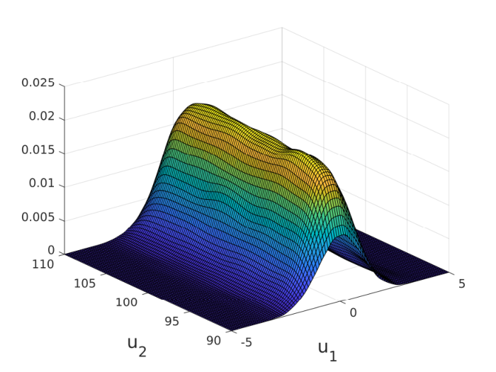
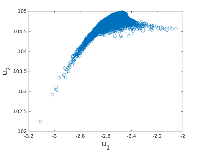
The second numerical experiment is a slightly modified example proposed in [21]. We consider a one-dimensional elliptic boundary value problem given by
with boundary conditions and , where is the unknown control. The exact solution of this problem is given by
where and . In the following example we consider , and , so that the explicit solution is given by
We assume to have noisy measurements of at the points and with value . The goal is to seek the control based on the knowledge of , of the prior and of the noise model. More precisely, we consider a prior information given by and a Gaussian white noise , with and begin the identity matrix. Thus, as in Section 5.1, noisy observations are simulated by
where the forward model is defined as
The example has dimension of the control in order to make a comparison between the solution to the inverse problem provided by the kinetic method and by the Bayes’ formula. In particular, it is possible to analyze the approximation of the mean estimator and of the posterior distribution computed by the kinetic equation (22). However, observe that (22) is derived by assuming a linear forward operator but in this example the model is nonlinear. Thus, inspired by (5), we consider a small modification of the microscopic interaction rule (18) with identity matrix given by
in order to perform the simulations for the nonlinear model.
For this example, the true posterior mean is computed in [21] thanks to Bayes’ formula and it is given by . In Figure 7 we show the results provided by the kinetic model. The top row shows the density estimation of the sampling from the initial distribution (left plot) and the positions of the samples at the last iterations. Again, we use the discrepancy principle as stopping criterion. The middle row shows the marginals of and as relative frequency plots. The solution computed as the mean estimator of the kinetic distribution is is very close to the true posterior mean, as proved also by the plot of the residuals in the bottom left panel of Figure 7. The application of the original EnKF method provides which is less accurate, see also [21].
6 Conclusions
In this paper we have introduced a kinetic model for the solution to inverse problems. The kinetic equation has been derived as mean-field limit of the Ensemble Kalman Filter method for infinitely large ensemble. The introduction of a continuous equation describing the evolution of the probability distribution of the unknown control guarantees several advantages: information on statistical quantities of the solution, implicit regularization modeled by the initial distribution, analysis of the properties of the solution.
The derivation of the kinetic equation has also the advantage to provide a different interpretation of the method and a possibly different scheme using binary collisions with consequent computational gain for numerical simulations. This leads to a different scheme as well as a modified scheme as introduced in the paper. A linear stability analysis for the simple setting of a one dimensional control has showed that the modified method has only stable solutions. Numerical simulations have been performed in order to investigate the good performance of the kinetic equation in providing solutions to inverse problems.
Acknowledgments
The authors would like to thank the German Research Foundation DFG for the kind support within the Cluster of Excellence Internet of Production (IoP).
The authors also acknowledge support by DFG HE5386/14,15.
Giuseppe Visconti is member of the “National Group for Scientific Computation (GNCS-INDAM)”.
References
- [1] S. I. Aanonsen, G. Nævdal, D. S. Oliver, A. C. Reynolds, and B. Vallès. The Ensemble Kalman Filter in Reservoir Engineering–a Review. SPE Journal, 14(03):393–412, 2013.
- [2] G. Albi and L. Pareschi. Binary interaction algorithms for the simulation of flocking and swarming dynamics. Multiscale Model. Simul., 11(1):1–29, 2013.
- [3] A. Apte, M. Hairer, A. M. Stuart, and J. Voss. Sampling the posterior: An approach to non-Gaussian data assimilation. Phys. D, 230:50–64, 2007.
- [4] J. O. Berger. Statistical Decision Theory and Bayesian Analysis. Springer, 2nd edition, 1985.
- [5] D. Bianchi, A. Buccini, M. Donatelli, and S. Serra-Capizzano. Iterated fractional Tikhonov regularization. Inverse Problems, 31(5):055005, 2015.
- [6] D. Bloemker, C. Schillings, and P. Wacker. A strongly convergent numerical scheme from ensemble kalman inversion. SIAM J. Numer. Anal., 56(4):2537–2562, 2018.
- [7] D. Bloemker, C. Schillings, P. Wacker, and S. Weissman. Well Posedness and Convergence Analysis of the Ensemble Kalman Inversion. Preprint. arxiv:1810.08463, 2018.
- [8] H. Bobovsky and H. Neunzert. On a simulation scheme for the boltzmann equation. Math. Methods Appl. Sci., 8(2):223–233, 1986.
- [9] M. Burger and F. Lucka. Maximum a posteriori estimates in linear inverse problems with log-concave priors are proper Bayes estimators. Inverse Problems, 30:114004, 2014.
- [10] R. E. Caflisch. Monte Carlo and quasi-Monte Carlo methods. Acta Numerica, 1998:1–49, 1998.
- [11] J. A. Carrillo, M. Fornasier, G. Toscani, and F. Vecil. Mathematical Modeling of Collective Behavior in Socio-Economic and Life Sciences, chapter Particle, kinetic, and hydrodynamic models of swarming, pages 297–336. Modeling and Simulation in Science, Engineering and Technology. Birkhäuser Boston, 2010.
- [12] J. A. Carrillo, L. Pareschi, and M. Zanella. Particle based gPC methods for mean-field models of swarming with uncertainty. Commun. Comput. Phys., 25:508–531, 2019.
- [13] N. K. Chada and X. T. Stuart, A. M. Tong. Tikhonov regularization within ensemble Kalman inversion. arxiv.org/abs/1901.10382, 2019.
- [14] E. Cristiani, B. Piccoli, and A. Tosin. MS&A: Modeling, Simulation and Applications, volume 12, chapter Multiscale Modeling of Pedestrian Dynamics. Springer International Publishing, 2014.
- [15] M. Dashti and A. M. Stuart. The Bayesian Approach to Inverse Problems, pages 311–424. Springer International Publishing, 2016.
- [16] P. Del Moral, A. Kurtzmann, and J. Tugaut. On the stability and the uniform propagation of chaos of a class of Extended Ensemble Kalman-Bucy filters. SIAM J. Control Optim., 55(1):119–155, 2017.
- [17] P. Del Moral and J. Tugaut. On the stability and the uniform propagation of chaos properties of Ensemble Kalman-Bucy filters. Ann. Appl. Probab., 28(2):790–850, 2018.
- [18] L. Desvillettes. On asymptotics of the Boltzmann equation when the collisions become grazing. Transport Theor. Stat., 21(3):259–276, 1992.
- [19] R. J. DiPerna and P. L. Lions. On the Fokker-Planck-Boltzmann equation. Commun. Math. Phys., 120(1):1–23, 1988.
- [20] H. W. Engl, M. Hanke, and A. Neubauer. Regularization of inverse problems, volume 375. Springer Science and Business Media, 1996.
- [21] O. G. Ernst, B. Sprungk, and H.-J. Starkloff. Analysis of the ensemble and polynomial chaos kalman filters in bayesian inverse problems. SIAM/ASA J. Uncertain. Quantif., 3(1):823–851, 2015.
- [22] G. Evensen. Sequential data assimilation with a nonlinear quasi-geostrophic model using monte carlo methods to forecast error statistics. J. Geophys. Res, 99:10143–10162, 1994.
- [23] G. Evensen. Data assimilation: the ensemble Kalman filter. Springer Verlag, 2009.
- [24] M. Fornasier, J. Haskovec, and J. Vybíral. Particle systems and kinetic equations modeling interacting agents in high dimension. Multiscale Model. Simul., 9:1727–1764, 2011.
- [25] C. W. Groetsch. The theory of Tikhonov regularization for Fredholm equations of the first kind, volume 105. Pitman Advanced Publishing Program, 1984.
- [26] S.-Y. Ha and E. Tadmor. From particle to kinetic and hydrodynamic descriptions of flocking. Kinet. Relat. Models, 3(1):415–435, 2008.
- [27] P. C. Hansen. Rank-Deficient and Discrete Ill-Posed Problems: Numerical Aspects of Linear Inversion. SIAM, 1998.
- [28] M. Herty and C. Ringhofer. Averaged kinetic models for flows on unstructured networks. Kinet. Relat. Models, 4(4):1081–1096, 2011.
- [29] M. Iglesias. Iterative regularization for ensemble data assimilation in reservoir models. Computational Geosciences, 19(1):177–212, 2015.
- [30] M. Iglesias, K. Law, and A. M. Stuart. Analysis of the Ensamble Kalman methods for inverse problems. Inverse Problems, 29(4):045001, 2013.
- [31] M. Iglesias, K. Law, and A. M. Stuart. Evaluation of Gaussian approximations for data assimilation in reservoir models. Comput. Geosci., 17:851–885, 2013.
- [32] R. E. Kalman. A new approach to linear filtering and prediction problems. J. Basic Eng.-T. ASME, 1960.
- [33] E. Klann and Ramlau R. Regularization by fractional filter methods and data smoothing. Inverse Problems, 24(2):0125018, 2008.
- [34] E. Kwiatkowski and J. Mandel. Convergence of the square root ensemble Kalman filter in the large ensemble limit. SIAM/ASA J. Uncertain. Quantif., 3(1):1–17, 2015.
- [35] T. Lange and W. Stannat. On the continuous time limit of the ensemble Kalman filter. arxiv.org/abs/1901.05204, 2019.
- [36] K. J. H. Law and A. M. Stuart. Evaluating data assimilation algorithms. Mon. Weather Rev., 140:3757–3782, 2012.
- [37] K. J. H. Law, H. Tembine, and R. Tempone. Deterministic mean-field ensemble kalman filtering. SIAM J. Sci. Comput., 38(3), 2016.
- [38] F. Le Gland, V. Monbet, and V.-D. Tran. Large sample asymptotics for the ensemble Kalman filter. Research Report RR-7014, INRIA, 2009.
- [39] M. Lemou. Multipole expansions for the Fokker-Planck equation. Numer. Math., 78(4):597–618, 1998.
- [40] A. J. Majda and X. T. Tong. Performance of Ensemble Kalman filters in large dimensions. Commun. Pur. Appl. Math., 71(5):892–937, 2018.
- [41] C. Mouhot and L. Pareschi. Fast algorithms for computing the Boltzmann collision operator. Math. Comput., 75:1833–1852, 2006.
- [42] D. S. Oliver, A. C. Reynolds, and N. Liu. Inverse Theory for Petroleum Reservoir Characterization and History Matching. Cambridge University Press, 2008.
- [43] L. Pareschi and G. Russo. An introduction to Monte Carlo methods for the Boltzmann equation. In CEMRACS 1999 (Orsay), ESAIM Proc., volume 10, Paris, 1999. Soc. Math. Appl. Indust.
- [44] L. Pareschi and G. Toscani. Interacting Multiagent Systems. Kinetic equations and Monte Carlo methods. Oxford University Press, 2013.
- [45] L. Pareschi, G. Toscani, and C. Villani. Spectral methods for the non cut-off Boltzmann equation and numerical grazing collision limit. Numer. Math., 93(3):527–548, 2003.
- [46] C. Schillings and A. M. Stuart. Analysis of the Ensamble Kalman Filter for Inverse Problems. SIAM J. Numer. Anal., 55(3):1264–1290, 2017.
- [47] C. Schillings and A. M. Stuart. Convergence analysis of ensemble Kalman inversion: the linear, noisy case. Applicable Analysis, 97(1):107–123, 2018.
- [48] A. M. Stuart. Inverse problems: a Bayesian perspective. Acta Numer., 19:451–559, 2010.
- [49] G. Toscani. Kinetic models of opinion formation. Commun. Math. Sci., 4(3):481–496, 2006.
- [50] T. Trimborn, L. Pareschi, and M. Frank. Portfolio Optimization and Model Predictive Control: A Kinetic Approach. Preprint. arxiv:1711.03291, 2018.
- [51] C. Villani. Conservative forms of Boltzmann’s collision operator: Landau revisited. ESAIM Math. Model. Numer. Anal., 33(1):209–227, 1999.