Hedging and Pricing European-type, Early-Exercise and Discrete Barrier Options using an Algorithm for the Convolution of Legendre Series
Abstract
This paper applies an algorithm for the convolution of compactly supported Legendre series (the CONLeg method) (Hale and Townsend 2014a, cf.), to pricing/hedging European-type, early-exercise and discrete-monitored barrier options under a Lévy process. The paper employs Chebfun (Trefethen et al. 2014, cf.) in computational finance and provides a quadrature-free approach by applying the Chebyshev series in financial modelling. A significant advantage of using the CONLeg method is to formulate option pricing and option Greek curves rather than individual prices/values. Moreover, the CONLeg method can yield high accuracy in option pricing and hedging when the risk-free smooth probability density function (PDF) is smooth/non-smooth. Finally, we show that our method can accurately price/hedge options deep in/out of the money and with very long/short maturities. Compared with existing techniques, the CONLeg method performs either favourably or comparably in numerical experiments.
keywords
Convolution, Legendre series, European options, early-exercise options, discrete-monitored barrier options, Lévy process1 Introduction
Applying robust numerical techniques in option pricing/hedging and model calibration provides interesting research questions in financial markets. The techniques must be not only highly accurate, but also efficient.
Suppose we consider the well-known European vanilla option pricing formula driven by a stochastic stock price process
| (1) |
where denotes the option value at an initial date of and with a strike price of stands for a payoff function at the maturity of is the expectation operator under the risk-neutral measure, and are the log-price and state variable respectively, can be decomposed into and is the probability density function of the process, and finally is a risk-neutral interest rate.
In the aforementioned formula, can be seen as a convolution integral, more precisely a cross-correlation integral, and the fast Fourier transform method (FFT method), a numerical integration-based method, (Carr and Madan 1999, Lewis 2001, Lipton 2002, Chourdakis 2004, Jackson et al. 2008, Lord et al. 2008, e.g.,), is a popular method for pricing European vanilla options as well as more exotic options, such as the American option, under Lévy processes. This is because the characteristic function of the underlying dynamics can be easily transformed into a risk-free probability density function (PDF) via the FFT method. The seminal work of these papers leads to the extension of combining the FFT with other transformation methods, e.g., the Hilbert transform or Gaussian transform, in pricing exotic options under the (time-changed) Lévy process or stochastic volatility models (Broadie and Yamamoto 2003, Broadie and Yamamoto 2005, Feng and Linetsky 2008, Cai and Kou 2011, Wong and Guan 2011, Zeng and Kwok 2014, e.g.,). Within the same numerical integration-based framework, numerical quadrature methods, such as Gaussian quadrature, are proposed mainly by Andricopoulos et al. 2003, O’Sullivan 2005, Andricopoulos et al. 2007, Chen et al. 2014 and Su et al. 2017. The authors of these papers abbreviate their quadrature techniques as QUAD methods. The original QUAD method was introduced in Andricopoulos et al. 2003, Andricopoulos et al. 2007 and requires the transition density to be known in closed form, which is the case in, e.g., the Black-Scholes model and Merton’s jump-diffusion model. This requirement is relaxed in Chen et al. 2014 where the QUAD-FFT or QUAD-CONV method is proposed. The main idea is that the PDF can be recovered by inverting the characteristic function via the FFT method. This helps open up the QUAD method to a much wider range of models. The latest development of the method (Su et al. 2017) is to improve the calculation speed, precomputing and caching PDFs and then applying the extrapolation and smoothing techniques to the method. Under the general framework of the QUAD method, only Delta, an option Greek, is formulated via the first-order finite difference method (FD) (Andricopoulos et al. 2003). However, the accuracy of the first-order FD is debatable in the context. Furthermore, other kinds of the Greeks, e.g. Gamma or Theta, are not mentioned or developed yet in this literature. In addition to the QUAD methods, in recent years, Pachón 2018 has introduced the CHEB method, Clenshaw-Curtis quadrature based on an expansion of the integrand in terms of Chebyshev polynomials, for approximate European options with arbitrary payoffs. The method is one of the natural applications of Chebfun (Trefethen et al. 2014), an open-source software system for numerical computing with functions.
Beyond the FFT method and the QUAD method, Oosterlee and his collaborators have attracted considerable attention (Leentvaar and Oosterlee 2008, Fang and Oosterlee 2009a, Fang and Oosterlee 2009b, Fang and Oosterlee 2011, Zhang and Oosterlee 2013, Ruijter et al. 2015). In their work, they adopt the Fourier cosine series (COS) to price options or derivatives that have different contingency claims and are characterised by path dependence and/or early-exercise features. The implementation of these methods is relatively simple but elegant and is capable of pricing options under different stochastic processes as long as their characteristic function exists. The main achievement of these methods is that they can, in many cases (such as European options), maintain an exponential convergence rate when pricing options. Moreover, these methods are also able to accurately price options under infinite variation processes. The COS method requires an adequate computational domain a priori, and, due to the recursion in time, errors caused by an inadequate domain propagate, resulting in incorrect option prices in the COS method. Moreover, based on the framework of the COS method, Oosterlee and his collaborators further apply the wavelet method called the Shannon wavelet inverse Fourier technique (SWIFT) method to price European, spread, path-dependent and discrete barrier options under exponential Lévy dynamics (Ortiz-Gracia and Oosterlee 2013, Ortiz-Gracia and Oosterlee 2016, Colldeforns-Papiol et al. 2017, e.g.,). The SWIFT method is used to circumvent the ineffectiveness of using the COS method to price early-exercise options. Nevertheless, comparing with the COS method, a theoretical proof is still lacking to show exponential convergence for the SWIFT method since the wavelet scale a parameter to adjust the accuracy of the method, is still chosen heuristically for achieving exponential convergence. Furthermore, the literature on SWIFT methods does not consider computation of Greeks.
In this manuscript we propose the CONLeg method, which uses Chebyshev and Legendre series to approximate a convolution, to improve the ineffectiveness of using the aforementioned methods. First, as mentioned in Fang and Oosterlee 2009a, Fang and Oosterlee 2009b and Chan 2018, the FFT-driven methods, like the CONV method (Lord et al. 2008), are computationally expensive to price option prices or to approximate the PDFs because a relatively large number of Fourier terms is required to obtain sufficient accuracy (see Table 5 in Section 6). Second, we question whether any kind of quadrature method is an effective method to approximate option prices/hedging values when option/hedging pricing formulae are treated as convolution integrals. Hale and Townsend 2014b suggest that since a convolution integral appears as a trapezoid (cf. Fig 1), more quadrature weights and abscissae are required to approximate the areas towards the left and right vertices of the trapezoid. Third, we want to provide a method that can work with any stochastic process with or without a closed-form PDF. For example, the COS and SWIFT methods only work very well when the process has a characteristic function and without applying the FFT, the QUAD method only works well with a closed-form PDF. Fourth, comparing against the CONV, COS, QUAD and SWIFT methods, the CONLeg method provides an option pricing/hedging curve rather than an individual point value. Fifth, unlike the COS method, we can require a proper computational domain a priori in the CONLeg method when we apply it to price early-exercise options. Hence, the CONLeg method will not produce incorrect option prices when we calculate the option prices recursively backwards in time, as we allow a sufficient computational domain for calculation. Sixth, through our numerical experiments, we show that the CONLeg method can achieve high accuracy in option pricing and hedging when the risk-free smooth probability density function (PDF) is non-smooth, and can be an effective method to price/hedge options for long/short maturities. Seventh, to fit in the Chebfun framework, we lay out a closed-form transformation of the complex Fourier expression of a smooth PDF into Chebyshev series when the closed-form PDF is not available (cf. Appendix A). In the similar fashion, we also provide a solution, the Fourier–Padé method (cf. Appendix B), for approximating non-smooth PDFs. Eighth, through this paper, we are keen to promote the convenience of Chebfun (Trefethen et al. 2014) in financial modelling. Chebfun is a robust, open source MATLAB pack for computing with functions to 15 digits of accuracy. It contains several state of the art algorithms for Chebyshev and other orthogonal polynomials. Finally, the current CONLeg method is different to the previous literature prompted Chebyshev series and interpolants in option pricing/hedging (Gaß et al. 2018, Pachón 2018, cf.). As we have mentioned in the previous point, comparing with the CHEB method (Pachón 2018), the CONLeg method is quadrature-free and not limited in pricing/hedging European-type options. Also, unlike Gaß et al. 2018’s tensorized Chebyshev interpolation to computing Parametric Option Prices (POP), our method does not approximate option pricing curves which must be first precomputed by any numerical method, such as the Monte Carlo and the FFT methods, for some fixed parameter configurations, and then compute other option prices for arbitrary parameter constellations. On the contrary, for a set of fixed parameters, the CONLeg method directly generates an option pricing/hedging curve via approximating a convolution integral without applying other numerical methods for computing the integral first.
The remainder of this paper is structured as follows. Section 2 describes the algorithm for the convolution of Legendre series and how Legendre series can be efficiently computed using the relationship with Chebyshev series and the FFT. Section 3 introduces the financial stochastic models we examine in this paper. Section 4 describes the formulation of the CONLeg option pricing/Greek formulae for different styles of European options as well as Bermuda, American, and discrete monitored barrier options. Section 5 describes the choice of truncated integration intervals. Section 6 discusses, analyses, and compares the numerical results of the CONLeg method with those of other numerical methods discussed above. Finally, we conclude and discuss possible future developments in Section 7.
2 Convolution of Legendre Series
Convolution is a fundamental operation that arises in many fields, particularly in financial derivatives research (Carr and Madan 1999, Lewis 2001, Lipton 2002, Jackson et al. 2008, Lord et al. 2008, cf.), econometrics (Bondarenko 2003, Liu et al. 2016) and statistics (Hogg et al. 2004). Given two integrable functions, and , their convolution is a third function, , defined formally by the integral
| (2) |
In general, if both and are analytic (smooth) and periodic functions, the FFT method, which utilises the convolution theorem and the fast Fourier transform (FFT), is the best choice for approximating as the FFT approximations of and do not suffer the Gibbs phenomenon.
If we now consider and as two compactly supported outside of then the convolution aforementioned via the integral is given by
| (3) |
and for 11 1 Since convolution is a commutative operation, we consider that only and are in the same intervals.. Without losing any generality, we can visualise each value of by the diagram in Figure 1, and we split into the two pieces suggested by the diagram:
| (4) |
Here, we denote, once and for all, and as the left and right hand side of the convolution, respectively.
Based in (3), either or can be a non-periodic continuous function, the FFT approximations of and suffer the Gibbs phenomenon such that there is a permanent oscillatory overshoot in the neighbourhoods of the endpoints and Accordingly, to avoid the Gibbs phenomenon, we adopt the algorithm proposed by Hale and Townsend 2014a to approximate The crucial idea of the algorithm is to approximate and with finite Legendre series and then convolve the approximations using the convolution theorem for them. The result is a piecewise polynomial representation that can be evaluated at any in the domain of to yield an approximation to . If the polynomials used to approximate and have degree at most , their algorithm produces an approximation to in operations. We summarise the approach below.
To illustrate Hale and Townsends’ algorithm of a convolution of two Legendre series, we first define the Legendre series on and then generalise to intervals Legendre polynomials, invented by Adrien-Marie Legendre, are the polynomial solutions to Legendre’s differential equation
| (5) |
with and integer parameter forms a polynomial sequence of orthogonal polynomials of degree and it can be expressed through Rodrigues’ formula:
| (6) |
Suppose we have and as two finite Legendre series on of degrees and with coefficients of and then we may write and as
| (7) |
With equal to the convolution in becomes
| (8) |
From (4), , consists of two pieces, on the left with and on the right with , each of degree We construct and by computing their Legendre coefficients. We focus on the computation of since that of is similar.
Denote by the vector of the Legendre coefficients of such that
| (9) |
By the orthogonality of Legendre polynomials and the orthonormalisation constant for for we have for for that
| (10) | ||||
| (11) |
Hale and Townsend 2014a prove that the above relation can be expressed in matrix form as Importantly (Hale and Townsend 2014a), there is a three-term recurrence relation of such that
| (12) | ||||
| (13) | ||||
| (14) |
where and both and can be computed in operations, and the whole matrix, , in operations. The matrix-vector product can be computed with the same cost and, accordingly, the coefficients of in operations. The coefficients of can be computed from , for which a nearly identical recurrence relation can be derived left since the computation for is similar.
Now, we direct our attention to the convolution of two finite Legendre series defined on the same interval We can define the composition of where is the linear mapping from to Apart from this, the Legendre series of and on respectively, are formulated by
| (15) |
(Hale and Townsend 2014a, Lemma 4.2). The convolution of of two continuous functions of and defined on can be computed as
| (16) |
where and
The approach above is not restricted to and on the same intervals. In contrast, the algorithm allows and which are polynomials of finite degree with zero support outside of and respectively. In this case (3) becomes
| (17) |
Depending on the difference between the length of and these are three different ideas to compute (17) on these subintervals of . For the full detail of computing on these subintervals, we refer interested readers to Hale and Townsend 2014a. The algorithm of convolution of Legendre series supported on same/general intervals is fully implemented as conv in Chebfun22 2 The algorithm in actually computes the convolution between two Chebyshev series by using fast Chebyshev-Legendre transform (Townsend et al. 2018) implemented in cheb2leg..
3 Lévy Processes
In this section, we briefly introduce the important properties of one-dimensional Lévy processes. Standard references for the stochastic processes can be found in Schoutens 2003 and Cont and Tankov 2004. Since markets are frictionless and have no arbitrage, we assume that an equivalent martingale measure (EMM) is chosen by the market. Moreover, there is a complete filtered probability space on which all processes are assumed to live.
3.1 Lévy processes
With and as the constant risk-free interest rate and the constant dividend yield, respectively, we describe a stock process driven by an exponential Lévy process such that
where and has infinitely divisible marginal distributions. Given a random variable we can define it as the corresponding characteristic function as follows:
| (18) |
If we define a truncation function which is a measurable function such that for every the characteristic function of can be described by the Lévy–Khinchine representation such that
| (19) |
Here, and are Lévy measures on which do not depend on the choice of (but note that depends on the choice of it). The condition that is a martingale will be guaranteed as long as an appropriate choice of the mean-correcting compensator is calculated as follows:
| (20) |
There are a substantial number of Lévy process examples in financial modelling. In this paper, we focus on geometric Brownian motion (GBM), variance gamma (VG), normal inverse Gaussian (NIG) and the Carr–Geman–Madan–Yor process (CGMY). Their characteristic functions can be defined as follows:
| (21) | ||||
| (22) | ||||
| (23) | ||||
| (24) |
Remark 3.1
Most Lévy processes do not have a closed-form representation of their risk-natural probability density function (PDF) ; however, some of the processes, e.g. GBM, NIG and VG, have a closed-formed PDF given by:
| (25) | ||||
| (26) | ||||
| (27) |
respectively. Here, is a modified Bessel function of a second kind, is a gamma function, , and
4 Pricing and Hedging Option via Convolution of Legendre Series
In this section, we apply the algorithm for the convolution of Legendre series to formulate option pricing/hedging formulas.
4.1 Pricing Formulae for European Type Options
Given the current log price the strike price of and maturity and the probability density function (PDF) of a stochastic process, we can express the option price starting at time with its contingent claim paying out as follows:
| (28) |
By replacing with , we have
| (29) |
where is the pay-off in log-price coordinates and is the reflected PDF function.
If is a piecewise continuous function, as is standard for most options, e.g., vanilla put and call, then applying the FFT method for a convolution function33 3 The expression of in (4.1) is indeed a cross-correlation integral; however, since we introduce the idea of the reflected function , we can turn (4.1) into a convolution integral instead., in will cause Gibbs phenomenon and as a result, will affect the accuracy of approximating . To avoid Gibbs phenomenon and allow a good approximation of we replace with an interval and employ the CONLeg method. The choice of satisfies the condition of
| (30) |
where is a characteristic function of Then we can approximate the pricing formula on i.e.,
| (31) |
where, has compact support outside of The final form of (4.1) is ready for approximating via the CONLeg method.
Most of the closed-form expressions of do not exist in the stochastic processes. If they do not, we adopt the ideas proposed in Chan 2016, Chan 2018 to express in a complex Fourier series (CFS) representation such that is approximated by:
| (32) |
where is a complex number and is the real part of a complex number, and given the condition of (30),
| (33) |
For the expression of we simply put a negative sign in the basis function i.e.,
| (34) |
If is smooth throughout on we can either directly approximate the CFS representation with a Chebyshev series using Chebfun (Trefethen et al. 2014, cf.) or transform it into a Chebyshev series using the techniques shown in Appendix A. If is a piecewise continuous function containing a singularity44 4 We refer a singularity as a point at which is not defined, or a point which fails to be well-behaved after differentiability, then we use the Fourier–Padé ideas to locate the singularity in and form accurate approximation. The details can be found in the Appendix B.
Knowing singularities in we divide and into a set of piecewise continuous functions and then approximate them with Chebyshev series using chebfun (cf. Trefethen et al. 2014, Chapter 1.4). Accordingly, we have a set of polynomials and each of degree at most and on the subintervals i.e.,
| (35) |
Here, as the indicator function in the interval and
| (36) |
Then, using the techniques implemented in cheb2leg (Townsend et al. 2018, cf.), we transform both and into Legendre series defined by
| (37) |
We use the algorithm for the convolution of Legendre series described in Section 2 to approximate their convolution on the subintervals Finally, transforming back into Chebyshev series using leg2cheb, can be approximated by
| (38) | ||||
| (39) | ||||
| where, | ||||
| (40) | ||||
Using (38), we can generate a set of option prices with a value of and a range of However, in the financial markets, option price quotes always appear with a value of and a range of To fit in this financial phenomenon, we modify (38) using the fact of so that we obtain the new pricing formula of
| (41) |
Remark 4.1
In Chebfun, there is a built-in algorithm to detect singularities automatically in a piecewise continuous function (Pachón et al. 2010, cf.). However, since PDFs can be easily expressed in the complex Fourier series and then extend to the Fourier–Padé series (Chan 2016, Chan 2018, cf.), we instead use Fourier–Padé ideas to locate singularities or approximate PDFs.
4.1.1 European Vanilla Call Options as illustration
We now consider pricing a European vanilla call, which can be exercised only at its maturity, defined in (4.1) with a payoff function of
| (42) |
We first transform the payoff into
| (43) |
By replacing with , we have a new form of denoted as
| (44) |
where and is a reflecting function. To make the CONLeg more efficient, we define a truncated computational interval (cf. Section 5), which satisfies condition to replace Then, is reformulated as
| (45) |
where To easily digest how the CONLeg method approximates , we assume that is a piecewise smooth function containing only one jump appearing in the payoff function, on . We can use chebfun to approximate and on 55 5 One should note that when . and respectively. Using the techniques described in Section 4.1, the European call option pricing formula is given by:
| (46) |
where, and
The CONLeg method is not limited from pricing European vanilla call option (4.1.1); it can be readily extended into a put option or other options with different pay-off structures, e.g., Cash-or-Nothing options. In Table 1, we list all financial contingency claims we consider in this paper and both their payoff functions and transformed payoff functions.
| Financial Contingency Claim | Payoff Function | Transformed Payoff Function |
|---|---|---|
| Call | ||
| Put | ||
| Covered Call | ||
| Cash-or-Nothing Call | ||
| Cash-or-Nothing Put | ||
| Asset-or-Nothing Call | ||
| Asset-or-Nothing Put | ||
| Asymmetric Call | ||
| Asymmetric Put |
4.2 Pricing Formulae for Bermuda Options
Consider now driven by a Lévy process and a Bermudan option with strike and maturity that can be exercised only on a given number of exercise dates We can write the Bermudan pricing formula for such an option as
| (48) |
where, is the payoff function at That is, if the payoff function is a call, then is transformed into In (48), at each can be defined as
| (49) |
To apply the CONLeg method to approximate we first understand that
| (50) |
is a martingale process. We also denote as and follow Section 4.1 to approximate as European option prices at . Then we can transform into
| (51) |
Since we approximate with the CONLeg method and use the Chebyshev series to present the Bermuda option prices accordingly, we can further modify (48) with a new form of
| (52) |
where Since the no-arbitrage assumption leads to the requirement that is continuous and at the early exercise curve, we must determine exercise point appearing in One way to do this is to use the Newton method proposed in Fang and Oosterlee 2009b to find However, since and are represented by piecewise smooth polynomials (chebfun), we can apply a built-in function roots in Chebfun to efficiently find these zeros. To do so, we first approximate as a Chebyshev series, then apply the roots function to find in the following equality:
Once we have and use it as a break point, we approximate
| (53) |
with two different Chebyshev series. Considering as a singularity and combining other singularities, e.g., singularities in a non-smooth PDF and/or in a payoff function, in we approximate with a set of Chebyshev series given by
| (54) |
Finally, summarising the methods above, we present the pseudo-code of our algorithm computing Bermudan option prices in Algorithm 1. A numerical example is also presented in Section 6.2.
4.3 Pricing Formulae for American Options
There are two basic approaches to evaluating American options based on our method for Bermudan options. As suggested in Fang and Oosterlee 2009b, one simple approach is to approximate an American option by a Bermudan option with many exercise opportunities. In other words, increase the number of exercise opportunities to a very large value. An alternative approach is to use Richardson extrapolation on a series of Bermudan options with an increasing number of (Geske and Johnson 1984, Chang et al. 2007, cf.). We adapt the latter approach (which is also implemented in Fang and Oosterlee 2009b) to price the American option here. Therefore, implementing the 4-point Richardson extrapolation scheme (Fang and Oosterlee 2009b, cf.), we have the American option price given by
| (55) |
where denotes the approximated value of the American option and is the pricing formulae for Bermudan options in (52).
4.4 Pricing Formulae for Discretely Monitored Barrier Options
A barrier option is an early-exercise option whose payoff depends on the stock price crossing a pre-set barrier level during the option’s lifetime. We call the option an up-and-out, knock-out, or down-and-out option when the option’s existence fades out after crossing the barrier level. Like European vanilla options, these options can all be written as either put or call contracts that have a pre-determined strike price on an expiration date. In this paper, we only investigate two basic types of barrier options.
- 1.
Down-and-out barrier (DO) option: A down-and-out barrier option is an option that can be exercised at a pre-set strike price on an expiration date as long as the stock price that drives the option does not go below a pre-set barrier level during the option’s lifetime. As an illustration, if the stock price falls below the barrier, the option is “knocked-out” and immediately carries no value.
- 2.
Up-and-out barrier (UO) option: Similar to a down-and-out barrier option, an up-and-out barrier option will be knocked out when the stock price rises above the barrier level during the option’s lifetime. Once it is knocked out, the option cannot be exercised at a predetermined strike price on an expiration date.
The structure of discretely monitored barrier options is the same as that of Bermudan options. Instead of having a pre-set exercise date and an early-exercise point like Bermudan options, barrier options have a pre-set monitored date and a barrier level. In the case of Bermudan options, when the stock price goes across the early exercise point, a payoff occurs, and the option expires immediately. In the same manner, a barrier option knocks out immediately when the barrier level is crossed. The barrier level acts exactly the same as the exercise point in Bermudan options. However, in the case of a barrier option without a rebate, no payoff occurs when the barrier level is reached; otherwise, a rebate occurs when a barrier option is knocked out.
We use a rebate DO option to illustrate the CONLeg method to approximate discretely monitored barrier option prices. Suppose that we have a rebate DO option driven by with a barrier , a rebate a strike and a series of monitoring dates : the option formulae can be described as
| (56) |
where is an indicator function and is again either a call or put payoff. We follow the ideas of (4.2) and (52) in Section 4.2 to approximate such that
| (57) |
After we apply the CONLeg method, (56) can be transformed into
| (58) |
In (58), since there is a jump at the barrier, at , we use as a break point and approximate
| (59) |
with two Chebyshev series. Moreover, combining other singularities in , we can formulate with a set of Chebyshev series given in (54). Finally, the pseudo-code of our algorithm calculating discretely monitored DO barrier option prices can be found in Algorithm 2.
4.5 Hedging Formulae and Choice of Truncated Intervals
We now turn our attention to deriving the option Greek values. In particular, we focus on deriving three option Greek values—Delta (), Gamma (), and Vega. Delta is defined as the rate of change in the option value with respect to changes in the underlying asset price; Gamma is the rate of change of Delta with respect to changes in the underlying price; and finally, Vega is the measurement of an option’s sensitivity to changes in the volatility of the underlying asset price. In general, volatility measures the amount and speed at which the price moves up and down and is often based on changes in the recent, historical prices of a trading instrument. Other Greek values, such as Theta, can be derived in a similar fashion; however, depending on the characteristic function, the derivation expressions might be rather lengthy. We omit them here, as many terms are repeated.
As mentioned above, Delta is the first derivative of the value of the option with respect to the underlying instrument price . Hence, differentiating the convolution form of in European options (38), Bermuda options (54), American options (55) and barrier options (54) with respect to we have
| (61) |
Since and simply becomes
| (62) | ||||
| with | ||||
| (63) | ||||
To express the first derivative of the Chebyshev series in (63), we adopt the fact of
(cf. Mason and Handscomb 2002, (2.4.5)) and such that we have
| (64) |
In a similar fashion, we can obtain by differentiating with respect to such that
| (65) |
To find we may use
(cf. Mason and Handscomb 2002, Problem 2.5.17), and thus find
| (66) |
and
| (67) |
Likewise, we can obtain the formula for Vega, where is the initial value of the volatility at time For example, for the GBM model with as the initial value of the volatility, we derive Vega as follows:
| (68) |
After we differentiate with respect to to obtain (68), we can approximate (68) with the CONLeg method.
If the closed-formed PDF of the stochastic process does not exist, as we mentioned before, we express with the CFS expression such that
| (69) |
where contains the parameter
5 Choice of Truncated Intervals
In this section, we adopt the ideas of Fang and Oosterlee 2009a and Chan 2018 to choose the interval . The choice of the interval plays the crucial role in the accuracy of the CONLeg method. If the choice of is too big, the CONLeg method can perform inefficiently. On the contrast, if is too small, the CONLeg method can produce inaccurate option prices/hedging values. Accordingly, a minimum and substantial interval can be chosen to capture most of the mass of a PDF such that our algorithm can in turn yield the highest accuracy. In this short section, we show how to construct an interval related to the closed-form formulas of stochastic process cumulants. The idea of using the cumulants is first proposed by Fang and Oosterlee 2009a to construct the definite interval in (30). Based on their ideas, we have the following expression for :
| (70) |
where and are the first, second and fourth cumulants, respectively, of the stochastic process and For simple, less-complicated financial models, we also obtain closed-form formulas for and , which are shown in Table 2.
| Lévy models | cumulants |
|---|---|
| BS | |
| NIG | |
| VG | |
In general, the truncated intervals in (5) work for smooth/non-smooth PDFs with/without singularities. However, as the cumulants in each process in Table 2 contain , we notice that if is too small, the cumulants shrink and make too small for the CONLeg to produce accurate option prices/hedging values. To solve the problem heuristically, as long as is less than or equal to we should add extra 0.5 to in (5) in order to produce a substantial interval for the CONLeg method.
6 Numerical Results
The main purpose of this section is to test the accuracy and efficiency of the CONLeg method through various numerical tests. This involves the ability of the method to price any options that are deep in/out of the money and have long/short maturities. Most importantly, we show that the algorithm exhibits good accuracy even when the PDF is smooth/non-smooth. A number of popular numerical methods are implemented to compare the algorithm in terms of the error convergence and computational time. These methods include the COS method (a Fourier COS series method, Fang and Oosterlee 2009a), the filter-COS method (a COS method with an exponential filter to resolve the Gibbs phenomenon; see Ruijter et al. 2015), the CONV method (an FFT method, Lord et al. 2008), the Lewis-FRFT (a fractional FFT method, Lewis 2001, Chourdakis 2004), the QUAD-CONV (a combination of the quadrature and CON methods; see O’Sullivan 2005, Chen et al. 2014), and the SWIFT methods (a wavelet-based method; see Ortiz-Gracia and Oosterlee 2013, Maree 2015, Ortiz-Gracia and Oosterlee 2016, Maree et al. 2017). When we implement the CONV and Lewis-FRFT methods, we use Simpson’s rule for the Fourier integrals to achieve fourth-order accuracy. In the filter-COS method, we use an exponential filter and set the accuracy parameter to as Ruijter et al. 2015 report that this filter provides better algebraic convergence than the other options. We also set the damping factors of the CONV to 0 for pricing European options. A MacBook Pro with a 2.8 GHz Intel Core i7 CPU and two 8 GB DDR SDRAM (cache memory) is used for all experiments. Finally, the code is written in MATLAB and also the codes of implementing the COS method and the FFT method, such as the CONV method and the like, is retrieved from von Sydow et al. 2015.
Since we use the built-in Chebfun (Trefethen et al. 2014) commands, mainly chebfun, conv, diff, roots and simplify, to price and hedge the options in this paper, Chebfun (http://www.chebfun.org/download/) is required for our option pricing algorithm. For a demonstration, we give the MATLAB code for computing European options in Appendix C. As Chebfun makes use of adaptive procedures that aim to find the right number of points automatically so as to represent each function to roughly machine precision, that is, about 15 digits of relative accuracy, we allow Chebfun to approximate and automatically. As Chebfun is implemented in MATLAB, we should point out that since Chebfun calls functions, nested functions and sub-functions considerably, the overheads occur and accordingly, this slows the CONLeg method’s computation speed down. Hence, as an introductory of the CONLeg method, we weigh more on the convenience of the method over its efficiency at this stage of development.
In all numerical experiments, the range of option prices we measure is based on the input range of or To allow our method to have accurate approximation of deep in/out-of-money option prices, the range of or lie in the intervals or respectively. Moreover, as we look at the intervals of or we set rather than for approximate option prices and their option Greek values 66 6 To achieve this, we can set a flag–“same”–in conv. See Appendix C for details..
We use to define the number of terms/grid points of the methods we compare against the CONLeg method. When measuring approximation errors of the numerical methods, we use absolute errors, the norm errors and the infinity norm errors as the measurement units. Moreover, to improve the accuracy of our method in pricing/hedging European type options, we use the well-known call-put parity relationship,
| (71) |
to approximate call prices once we have put prices ready.
6.1 European Type Options
We consider three different test cases based on the following PDFs and other parameters:
| (72) | ||||
| (73) | ||||
| (74) |
In all three numerical tests, the reference values for the GBM process and the VG process are generated via MATLAB Financial Toolbox™–blsprice, blsdelta and blsgamma–and the Singularity Fourier–Padé (SFP) method (Chan 2018, cf.) respectively. We also set in (5) when we create a computational interval for pricing/hedging European options under the two processes.
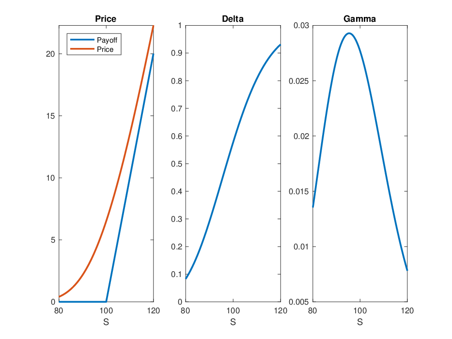
In the first numerical test (GBM1)–Table 3, we first check for convergence behaviour against a range of strikes from to for deep in/out-of-the money and at-the-money vanilla put options. Apart from the parameters are retrieved from von Sydow et al. 2015. We declare 1000 different option prices within the range of either In this test, even without applying the put-call parity (71), the CONLeg can achieve very high accuracy (around ) when it is applied to approximate option prices and its Delta and Gamma Moreover, since our method aims to model option price/Greek curves rather than their values, our method consumes only less than 0.1 seconds to formulate the curves in the test. Using around 0.1 seconds to produce option price and Greek curves is a quite reasonable computational cost for a method to meet the financial standards. The second numerical experiment (GBM2) is devoted to the performance of the CONLeg method for long maturity call options, which are often encountered in the insurance and pension industry. The parameters are retrieved from Ortiz-Gracia and Oosterlee 2016 for the test. Table 4 refers to the second test (GBM2) and replicates Table 3 in Ortiz-Gracia and Oosterlee 2016. In this test, with the help of (71), the CONLeg method impressively provides high accuracy when we declare 1000 different option prices within the range of from 80 to 120. The last set of parameters (VG1) is chosen in the last numerical test (Table 5) because relatively slow convergence was reported for the CONV method for very short maturities in Lord et al. 2008. This is attributed to the PDF of the process being sharp-peaked with a difficult logarithmic singularity (see Fig. 2). Before we approximate the closed-form VG PDF defined in (27) with Chebyshev series, we apply the Fourier–Padé method (cf. Appendix B) to locate the singularity in the PDF. We use as a breakpoint and approximate the PDF in two different regions and to resolve Gibbs phenomena. Since we use the Fourier–Padé method to approximate the PDF, the number of Fourier terms in the Fouier–Padé approximation is set to be 1024. In Table 5, again with the aid of (71), within similar CPU time and 30 options measured within the range of 80 and 90, the CONLeg method yields almost same accuracy to the COS and filter-COS methods, but relatively higher accuracy than the Lewis-FRFT, QUAD-CONV and CONV methods.
Remark 6.1
Fang and Oosterlee 2009a suggest that the VG process with VG1 gives rise to a probability density function that is not in , and thus, option pricing under VG with these parameter sets exhibits only an algebraic convergence. Nevertheless, Chan 2018 has recently proposed the SFP method to circumvent the problem and to approximate the VG PDF with the input parameters of VG1. Through this method, we can regain global spectral convergence away from singularities. For more details, we refer the readers to Chan 2018.
| Price | Delta | Gamma | ||||
| Time | ||||||
| 5.329e-14 | 3.921e-13 | 5.645e-14 | 1.846e-13 | 8.538e-13 | 1.396e-12 | 9.11e-02 |
| Price | Delta | Gamma | |||||
| Time | |||||||
| 2.842e-14 | 2.821e-13 | 2.220e-16 | 1.005e-15 | 7.170e-17 | 5.007e-16 | 8.34e-02 | |
| Time | |||||||
| 2.842e-14 | 2.874e-13 | 3.841e-16 | 2.123e-16 | 6.126e-19 | 3.776e-18 | 9.12e-02 | |
| Lewis-FRFT | CONV | QUAD–CONV | |||||||
| Time | Time | Time | |||||||
| 1024 | 9.921e-03 | 1.121e-02 | 0.092 | 1.217e-04 | 8.817e-03 | 0.110 | 2.411e-04 | 7.827e-03 | 0.121 |
| COS | filter-COS | CONLeg | |||||||
| Time | Time | Time | |||||||
| 1024 | 2.271e-06 | 7.579e-05 | 0.089 | 6.596e-07 | 3.596e-06 | 0.0912 | 5.596e-07 | 4.511e-06 | 0.102 |
6.2 American, Barrier and Bermuda Options
In this section we again focus on three test cases based on the following PDFs and other parameters:
| (75) | ||||
| (76) | ||||
| (77) |
In this section, as suggested by Fang and Oosterlee 2009b, we first set in (5) to create a computational interval for approximating the PDFs of the NIG and CGMY processes. In our first test we price Bermudan put options with 10 exercise dates with parameters of NIG1. In this test (Table 6), a total of 170 option prices are generated in the COS and CONV methods from a range of between 80 to 120. The CPU times are reported in seconds, and all reference values are obtained by the CONV method with Fang and Oosterlee 2009b report that the NIG PDF (26) is more peaked at the mean with the parameters of NIG1. We then use the mean as a breakpoint to approximate the PDF in two regions and From the result of Table 6, the accuracy of the COS method stays the same when increases from 256 to 512. Within the similar CPU time, we can see that the CONLeg has better accuracy than the COS method.
In the next two tests, the CGMY processes with parameters of CGMY1 and CGMY2 do not have a closed-form PDF and have singularities. Accordingly, again using the techniques we mentioned above, we use the Fourier–Padé method to approximate the CGMY PDFs and locate their singularities. The number of Fourier terms in the Fouier–Padé approximation is set to be 1024 in the tests.
The prices of American options can be obtained using (55), a 4-point Richardson extrapolation method on the prices of a few Bermudan options with small We compare the CONV, COS and CONLeg methods for pricing American option price in Table 7. All reference values are obtained by the Fourier time stepping method (Jackson et al. 2008) with the number of the Fourier terms equal to Within the similar CPU time, the CONLeg method achieves the same accuracy with the COS method and is marginally better than the CONV method.
For the last two tables, all reference values are obtained by the CONV method with In Table 8, we consider monthly monitored up-and-out call and put options, (UO Call) and (UO Put) under the CGMY process with the parameters of CGMY2. The barrier level is set to be 120 for the up-and-out options. As we can see from the table, the CONLeg method is very comparable to the SWIFT method in terms of accuracy. Finally, in Table 9, we focus on the NIG process with parameters of NIG1, except S=90–110 and K=100. Considering monthly monitored down-and-out call (DO Call) and put (DO Put) options, we set equal to 80 for the options. Since is very large, it causes the time interval difference between and to be very small. Accordingly, the NIG PDF is very peaked and the COS method requires a larger number of equal to 8192 to compensate a better convergence in Table 9. Comparing the CONLeg and COS methods in the similar CPU time, both methods can achieve similar accuracy.
| COS | CONLeg | |||||
| Time | Time | |||||
| 256 | 2.411e-07 | 5.411e-06 | 2.89 | 1.812e-13 | 8.576e-12 | 2.93 |
| Time | Time | |||||
| 512 | 2.411e-07 | 5.411e-06 | 3.323 | 1.812e-13 | 8.576e-12 | 2.93 |
| in Eq. (55) | CONV | CONLeg | |||||
|---|---|---|---|---|---|---|---|
| Time (sec.) | Time (sec.) | ||||||
| 2 | 32768 | 1.052e-04 | 8.051e-03 | 19.291 | 7.123e-05 | 6.113e-04 | 19.311 |
| in Eq. (55) | COS | CONLeg | |||||
| Time (sec.) | Time (sec.) | ||||||
| 2 | 32768 | 9.234e-05 | 4.012e-04 | 19.298 | 7.123e-05 | 6.113e-04 | 19.311 |
| SWIFT | CONLeg | ||||||
|---|---|---|---|---|---|---|---|
| Time (sec.) | Time (sec.) | ||||||
| UO Call | 6 | 3.181e-10 | 7.641e-09 | 7.100 | 5.186e-09 | 6.886e-08 | 7.201 |
| UO Put | 6 | 1.901e-11 | 8.621e-10 | 6.901 | 4.330e-10 | 6.131e-09 | 6.891 |
| COS | CONLeg | ||||||
|---|---|---|---|---|---|---|---|
| Time (sec.) | Time (sec.) | ||||||
| DO Call | 8192 | 6.701e-08 | 4.641e-07 | 94.231 | 4.167e-09 | 8.651e-08 | 93.812 |
| DO Put | 8192 | 7.232e-09 | 3.231e-08 | 92.532 | 1.619e-09 | 6.886e-08 | 92.634 |
7 Conclusions
In this paper, we have proposed an algorithm for hedging and pricing various options based on approximating probability density functions by polynomials (in particular, Legendre series) and computing the prices by performing suitable convolutions with the given payoff function. We call this method CONLeg. The main advantages of the CONLeg method are its ability to return the price and Greeks as a function defined on a prescribed interval rather than just point values, its ability to approximate different types options under a process with/without a closed-from PDF, and the simplicity and convenience of its implementation using Chebfun. We presented a proof of concept implementation written in Chebfun, which demonstrates positive results in the accuracy of the method. Since Chebfun uses adaptive approximations, it is difficult at this time to discuss rates of convergence of the CONLeg method or to compare it’s efficiency with respect to other methods in the literature (which work with a fixed discretisation size), but initial results are promising. For a fair comparison, one would need to implement a non-adaptive version of CONLeg, which would be time-consuming, and not typically desirable in a practical setting.
Our ultimate goal is to extend the method to price options with path-dependant features under the (time-changed) Lévy process or stochastic volatility with and without singularities. Research in this direction is already underway and will be presented in a forthcoming manuscript.
Appendix A A Closed-form Transformation of Complex Fourier Series into Chebyshev Series
To transform a complex Fourier series (CFS) into a Chebyshev series, we apply the result of Townsend 2014, i.e.
| (78) |
Here, is the Bessel functions of the first kind with parameter and is the Chebyshev polynomial of degree We first note that since a PDF, is a real function, the CFS representation of with a form of
| (79) |
can be interchangable into
| (80) |
Using (78) and (80), we may define a Chebyshev series on the same interval such that
where,
Appendix B Locating Singularities in Probability Density Functions
Many PDFs of interest are not smooth but piecewise smooth. For example, see Figure 2. If the locations of all singularities are not known in advance, we can use Fourier–Padé ideas (Driscoll and Fornberg 2011, Chan 2018, cf.) to estimate the locations of singularities well enough to allow good reconstruction nearly everywhere in the interval .
The Fourier–Padé algorithm proposed in this paper is very simple to implement. If we consider a function with a power series representation such that
and a rational function defined by where and are the polynomials of
| (82) |
respectively, then we say that is the (linear) Padé approximant of order (N, M) of the formal series satisfying the condition
| (83) |
Here, is approximated by To obtain the approximant we simply calculate the coefficients of polynomials and by solving a system of linear equations. To obtain we first normalise to ensure that the system is well determined and has a unique solution in (83). Then, we consider the coefficients for and we can yield a Toeplitz*77 7 A Toeplitz matrix or diagonal-constant matrix is an invertible matrix in which each descending diagonal from left to right is constant. linear system:
| (84) |
Once is known, is found through the terms of order N and less in (83). This yields , where . For example, if one obtains
| (85) |
Now, assuming is a PDF, to find singularities in and to express in a Fourier–Padé series, we first express with the CFS representation:
| (86) |
Then, we can differentiate (86) with respect to to obtain
| (87) |
Finally, we let in the two equations above, and they are ready for the Fourier–Padé approximation. In general, when the PDF has a singularity, the sharp-peaked singularity point will have an enormously large value after differentiation. In other words, Figure 2 is a graphical illustration of the outlooks of the PDF (left) and the first derivative (right) of the VG model after the Fourier–Padé approximation. In the figure, we can see that the non-smooth PDF with a jump can produces a value of at the singularity point after the first derivative. See padeapprox in Chebfun.

Appendix C MATLAB Code
C.1 Output
References
- Andricopoulos et al. (2003) Andricopoulos AD, Widdicks M, Duck PW, Newton DP (2003) Universal option valuation using quadrature methods. J. Financ. Econ. 67(3):447–471.
- Andricopoulos et al. (2007) Andricopoulos AD, Widdicks M, Newton DP, Duck PW (2007) Extending quadrature methods to value multi-asset and complex path dependent options. J. Financ. Econ. 83(2):471–499.
- Bondarenko (2003) Bondarenko O (2003) Estimation of risk-neutral densities using positive convolution approximation. J. Econom. 116(1):85–112.
- Broadie and Yamamoto (2003) Broadie M, Yamamoto Y (2003) Application of the fast Gauss transform to option pricing. Manage. Sci. 49(8):1071–1088.
- Broadie and Yamamoto (2005) Broadie M, Yamamoto Y (2005) A double-exponential fast Gauss transform algorithm for pricing discrete path-dependent options. Oper. Res. 53(5):764–779.
- Cai and Kou (2011) Cai N, Kou SG (2011) Option pricing under a mixed-exponential jump diffusion model. Manage. Sci. 57(11):2067–2081.
- Carr and Madan (1999) Carr P, Madan D (1999) Option valuation using the fast Fourier transform. J. Comput. Finance 4(2):61–73.
- Chan (2016) Chan TLR (2016) An orthogonal series expansions method to hedge and price European-type options. Available online at: https://papers.ssrn.com/sol3/papers.cfm?abstract_id=2852033.
- Chan (2018) Chan TLR (2018) Singular Fourier-Páde series expansion of European option prices. Quant. Finance 18(7):1149–1171.
- Chang et al. (2007) Chang CC, Chung SL, Stapleton RC (2007) Richardson extrapolation techniques for the pricing of American-style options. J. Futures Markets 27(8):791–817, ISSN 1096-9934.
- Chen et al. (2014) Chen D, Härkönen HJ, Newton DP (2014) Advancing the universality of quadrature methods to any underlying process for option pricing. J. Financ. Econ. 114(3):600–612.
- Chourdakis (2004) Chourdakis K (2004) Option pricing using the fractional FFT. J. Comput. Finance 8(2):1–18.
- Colldeforns-Papiol et al. (2017) Colldeforns-Papiol G, Ortiz-Gracia L, Oosterlee C (2017) Two-dimensional Shannon wavelet inverse Fourier technique for pricing European options. Appl. Numer. Math. 117:115–138, ISSN 0168-9274.
- Cont and Tankov (2004) Cont R, Tankov P (2004) Financial Modelling with Jump Processes. Chapman & Hall/CRC Financial Mathematics Series (Boca Raton, FL: Chapman & Hall/CRC).
- Driscoll and Fornberg (2011) Driscoll TA, Fornberg B (2011) The Gibbs Phenomenon in Various Representations and Applications (Potsdam, NY: Sampling Publishing).
- Fang and Oosterlee (2009a) Fang F, Oosterlee CW (2009a) A novel pricing method for European options based on Fourier-cosine series expansions. SIAM J. Sci. Comput. 31(2):826–848.
- Fang and Oosterlee (2009b) Fang F, Oosterlee CW (2009b) Pricing early-exercise and discrete barrier options by Fourier-cosine series expansions. Numer. Math. 114(1):27–62.
- Fang and Oosterlee (2011) Fang F, Oosterlee CW (2011) A Fourier-based valuation method for Bermudan and barrier options under Heston’s model. SIAM J. Financ. Math. 2(1):439–463.
- Feng and Linetsky (2008) Feng L, Linetsky V (2008) Pricing discretely monitored barrier options and defaultable bonds in Lévy process models: A fast Hilbert transform approach. Math. Financ. 18(3):337–384.
- Gaß et al. (2018) Gaß M, Glau K, Mahlstedt M, Mair M (2018) Chebyshev interpolation for parametric option pricing. Finance Stoch. 22(3):701–731.
- Geske and Johnson (1984) Geske R, Johnson HE (1984) The American put option valued analytically. J. Finance 39(5):1511–1524.
- Hale and Townsend (2014a) Hale N, Townsend A (2014a) An algorithm for the convolution of Legendre series. SIAM J. Sci. Comput. 36(3):A1207–A1220.
- Hale and Townsend (2014b) Hale N, Townsend A (2014b) A fast, simple, and stable Chebyshev–Legendre transform using an asymptotic formula. SIAM J. Sci. Comput. 36(1):A148–A167.
- Hogg et al. (2004) Hogg RV, McKean JW, Craig AT (2004) Introduction to Mathematical Statistics (New Jersey: Prentice Hall), 6 edition.
- Jackson et al. (2008) Jackson KR, Jaimungal S, Surkov V (2008) Fourier space time-stepping for option pricing with Lévy models. J. Comput. Finance 12(2):1–29.
- Leentvaar and Oosterlee (2008) Leentvaar C, Oosterlee C (2008) Multi-asset option pricing using a parallel Fourier-based technique. J. Comput. Finance 12(1):1–26.
- Lewis (2001) Lewis A (2001) A simple option formula for general jump-diffusion and other exponential Lévy processes. Available online at: http://optioncity.net/pubs/ExpLevy.pdf.
- Lipton (2002) Lipton A (2002) The vol smile problem. Risk 15:61–66.
- Liu et al. (2016) Liu X, Xiao H, Chen R (2016) Convolutional autoregressive models for functional time series. J. Econom. 194(2):263–282.
- Lord et al. (2008) Lord R, Fang F, Bervoets F, Oosterlee CW (2008) A fast and accurate FFT-based method for pricing early-exercise options under lévy processes. SIAM J. Sci. Comput. 30(4):1678–1705.
- Maree (2015) Maree SC (2015) Numerical pricing of Bermudan options using Shannon wavelet expansions. Master’s thesis, Delft Institute of Applied Mathematics, Delft University of Technology, Delft, The Netherlands.
- Maree et al. (2017) Maree SC, Ortiz-Gracia L, Oosterlee CW (2017) Pricing early-exercise and discrete barrier options by Shannon wavelet expansions. Numer. Math. 136(4):1035–1070, ISSN 0029-599X.
- Mason and Handscomb (2002) Mason JC, Handscomb D (2002) Chebyshev Polynomials (Florida, FL, USA: CRC Press).
- Ortiz-Gracia and Oosterlee (2013) Ortiz-Gracia L, Oosterlee CW (2013) Robust pricing of European options with wavelets and the characteristic function. SIAM J. Sci. Comput. 35(5):B1055–B1084.
- Ortiz-Gracia and Oosterlee (2016) Ortiz-Gracia L, Oosterlee CW (2016) A highly efficient Shannon wavelet inverse Fourier technique for pricing European options. SIAM J. Sci. Comput. 38(1):B118–B143.
- O’Sullivan (2005) O’Sullivan C (2005) Path dependant option pricing under Lévy processes. EFA 2005 Moscow Meetings Paper, 24.
- Pachón (2018) Pachón R (2018) Numerical pricing of European options with arbitrary payoffs. Int. J. Financ. Eng. 5(2):1850015.
- Pachón et al. (2010) Pachón R, Platte RB, Trefethen LN (2010) Piecewise-smooth chebfuns. IMA J. Numer. Anal. 30(4):898–916.
- Ruijter et al. (2015) Ruijter M, Versteegh M, Oosterlee C (2015) On the application of spectral filters in a Fourier option pricing technique. J. Comput. Finance 19(1):75–106.
- Schoutens (2003) Schoutens W (2003) Lévy Processes in Finance: Pricing Financial Derivatives. Wiley Series in Probability and Mathematical Statistics (Chichester, UK: Wiley).
- Su et al. (2017) Su H, Chen D, Newton DP (2017) Option pricing via QUAD: From Black-Scholes-Merton to Heston with jumps. J. Deriv. 24(3):9–27.
- Townsend (2014) Townsend A (2014) Computing with functions in two dimensions. Thesis, University of Oxford, Oxford, UK, see http://math.mit.edu/˜ajt/papers/thesis.pdf.
- Townsend et al. (2018) Townsend A, Webb M, Olver S (2018) Fast algorithms for Toeplitz and Hankel matrices. Mathematics of Computation 87(1):1913–1934.
- Trefethen et al. (2014) Trefethen LN, Driscoll TA, Hale N (2014) Chebfun Guide (Oxford: Pafnuty Publications), see http://www.chebfun.org/.
- von Sydow et al. (2015) von Sydow L, Höök LJ, Larsson E, Lindström E, Milovanović S, Persson J, Shcherbakov V, Shpolyanskiy Y, Sirén S, Toivanen J, Waldén J, Wiktorsson M, Levesley J, Li J, Oosterlee CW, Ruijter MJ, Toropov A, Zhao Y (2015) BENCHOP–the BENCHmarking project in option pricing. Int. J. Comput. Math. 92(12):2361–2379.
- Wong and Guan (2011) Wong HY, Guan P (2011) An FFT-network for Lévy option pricing. J. Bank. Finance 35(4):988–999.
- Zeng and Kwok (2014) Zeng P, Kwok YK (2014) Pricing barrier and Bermudan style options under time-changed Lévy processes: Fast Hilbert transform approach. SIAM J. Sci. Comput. 36(3):B450–B485.
- Zhang and Oosterlee (2013) Zhang B, Oosterlee CW (2013) Efficient pricing of European-style Asian options under exponential Lévy processes based on Fourier cosine expansions. SIAM J. Financ. Math. 4(1):399–426.