Experimental demonstration of quantum advantage for one-way
communication complexity
Abstract
The goal of demonstrating a quantum advantage with currently available experimental systems is of utmost importance in quantum information science. While this remains elusive for quantum computation, the field of communication complexity offers the possibility to already explore and showcase this advantage for useful tasks. Here, we define such a task, the Sampling Matching problem, which is inspired by the Hidden Matching problem and features an exponential gap between quantum and classical protocols in the one-way communication model. Our problem allows by its conception a photonic implementation based on encoding in the phase of coherent states of light, the use of a fixed size linear optic circuit, and single-photon detection. This enables us to demonstrate experimentally an advantage in the transmitted information resource beyond a threshold input size, which would have been impossible to reach for the original Hidden Matching problem. Our demonstration has implications in various communication and cryptographic settings, for example for quantum retrieval games and quantum money.
Introduction
A major objective in quantum information science presently is finding communication and computational tasks for which it is possible to demonstrate in practice that using quantum instead of classical resources leads to superior performance in terms of computational power, security or communication efficiency. In the quest for such demonstrations for computational tasks Harrow and Montanaro 2017, significant achievements include Boson Sampling Aaronson and
Arkhipov 2011; Neville et al. 2017, which has been implemented for small sizes Broome et al. 2013; Tillmann et al. 2013; Crespi et al. 2013; Spagnolo et al. 2014, and sparse commuting (IQP) or random quantum circuits Farhi and Harrow 2016; Bremner et al. 2017; Bravyi et al. 2017; Gao et al. 2017; Bermejo-Vega et al. 2018; Aaronson and Chen 2016; Boixo et al. 2018. Another recent proposal deals with the power of quantum interactive proofs for verifying NP-complete problems with small proofs Aaronson et al. 2008; Arrazola et al. 2018.
Concerning communication tasks, there have been several works demonstrating security impossible to achieve by classical means, including quantum key distribution Scarani et al. 2009; Diamanti et al. 2016 and several other cryptographic primitives in various configurations Donaldson et al. 2016; Pappa et al. 2014; Barz et al. 2012; McCutcheon et al. 2016, or involving non-local games that rely on the violation of Bell inequalities Hensen et al. 2015; Pappa et al. 2015.
In addition to increased security, quantum technologies can also provide an advantage in terms of communication and information resources, such as the amount of information that needs to be transmitted to jointly perform a distributed task between two or more parties who each receive an input, or the total time this takes. Calculating and optimizing the use of such resources is the goal of the field of communication complexity, where protocols typically either minimize the amount of information that needs to be exchanged to solve a problem with certainty or maximize the probability of solving the problem successfully using a restricted amount of communication. This field has a great range of applications including, for instance, the optimization of very large scale integrated circuits or data structures. It has been shown that quantum resources lead to exponential asymptotic savings compared to classical resources for several protocols Buhrman et al. 2001; Buhrman et al. 1998; Raz 1999; Gavinsky et al. 2007; Gavinsky 2016; Regev and Klartag 2011, including the Hidden Matching protocol Bar-Yossef et al. 2004 used in our work. The underlying factor that enables this advantage is that while in classical networks such tasks require a very large amount of information exchange, when quantum resources are available it is sufficient for one of the parties to generate, locally manipulate and send specific states called quantum fingerprints. However, these are highly entangled multi-qubit states of large dimension, whose generation is out of reach of experimental photonic technologies currently used in quantum communications.
A significant step in the direction of experimental quantum communication complexity was made by theoretical work proposing a mapping for encoding quantum communication protocols involving pure states of many qubits, unitary operations and projective measurements to protocols based on coherent states of light in a superposition of optical modes, linear optics operations and single-photon detection Arrazola and Lütkenhaus 2014a. This model was used to propose the practical implementation of coherent state quantum fingerprints for computing the Equality function in the simultaneous message passing model of communication complexity Arrazola and Lütkenhaus 2014b, leading to experiments demonstrating a quantum advantage in the transmitted information in this model Xu et al. 2015; Guan et al. 2016. Further work proposed a model involving multiplexed coherent state fingerprints to improve not only the information resource but also the communication resource Kumar et al. 2017. We also remark that a communication complexity advantage in time was experimentally shown recently for the quantum switch resource used in indefinite causal structures Wei et al. 2018.
Here, we define a new communication task and experimentally demonstrate a quantum advantage in the one-way communication complexity model, where only one party is allowed to send a message to a second one, who outputs a solution to the task – a model particularly suitable for applications in quantum networks. More precisely, based on the Hidden Matching problem introduced in Ref. Bar-Yossef et al. 2004, we define the Sampling Matching problem, for which we show that it remains a hard problem for classical one-way communication while there is a quantum protocol that is exponentially more efficient with respect to the transmitted information than any randomized classical protocol with bounded error. We then apply the aforementioned coherent state mapping to Sampling Matching and we show that its implementation in this framework requires a constant number of linear optic components, contrary to the original Hidden Matching problem that would require a large number of active components increasing with the input size of the problem. The conception of Sampling Matching was inspired by a passive implementation of the round robin differential phase shift quantum key distribution (RR-DPS-QKD) protocol Sasaki et al. 2014; Guan et al. 2015, which trades simplicity and stability of the experimental setup with the need for remote phase locking in a full-scale implementation. In our case, exploiting these concepts allows us to use a state-of-the-art photonic system involving encoding in the phase of weak coherent states, linear optics and single-photon detection, for a proof-of-principle implementation of Sampling Matching, which outperforms the best known classical protocol with respect to the transmitted information from threshold input size of around 3000. Such a quantum advantage for one-way communication complexity would have been impossible to reach previously, hence our experiment paves the way to the demonstration of a number of useful communication tasks that rely on similar principles.
Results
Hidden Matching.
Let us start by describing the Hidden Matching problem as it was defined in Ref. Bar-Yossef et al. 2004 and its translation into the coherent state mapping framework of Ref. Arrazola and
Lütkenhaus 2014a. We will then outline the linear optic circuit necessary for implementing this protocol, which will showcase the need for defining a new problem to be able to drastically reduce the resources required for demonstrating a quantum advantage in the model of one-way communication complexity.

The Hidden Matching problem is illustrated in Fig. 1. It is a one-way communication complexity task involving two players, Alice and Bob, and is described as follows. For any positive even integer , Alice receives as input a string while Bob receives a perfect matching uniformly at random from a set . Here is a set of perfect edge-disjoint matchings on nodes. An example for is shown in Fig. 2. The objective of the problem is for Bob to output any one of the possible parity values for a pair that belongs to the matching with minimum communication and information resources. Here are the and bit of respectively. We analyse this problem in the randomized setting where Bob is allowed to use random coins and output the correct value with high probability. This problem further imposes the restriction of communication only from Alice to Bob otherwise it is easy to see that the task can be done with logarithmic communication, since Bob can send to Alice the indices and Alice will reply with the parity.

Classical strategy. For this problem, the randomized classical lower bound of was shown by Bar-Yossef et al. Bar-Yossef et al. 2004 and later extended by Buhrman et al. Buhrman et al. 2011. The main idea is that Alice’s message should allow Bob to output the parity of an edge from each one of the possible matchings, in other words for different edges. No matter which edges one picks, they will always contain at least different bits of the input , and hence Alice must send at least bits of information and hence communication. The proof structure for computing the lower bound is as follows Buhrman et al. 2011: if Alice’s message to Bob is small, let’s say bits, then the set of inputs for which Alice sends a particular message will be large (typically of the order of ). This would mean that Bob will have very little knowledge for most of the bits of . Using techniques from Ref. Kahn et al. 1988 this implies that Bob would not be able to correctly answer the parity for most of the possible tuples . Even though Bob has some relaxation in the sense that he can output the parity outcome of any one of the tuples of , still it turns out that on average it is hard for him to output the correct parity outcome. Using this idea, the classical lower bound to succeed with an error probability is,
| (1) |
Bar-Yossef et al. also proved that this bound is tight by describing a randomized one-way protocol using the birthday paradox argument to show that only classical bits are sufficient to solve the problem. The proof structure is as follows: Let us assume that Bob’s matching set is restricted to be one of the disjoint matchings. Since Alice has no information about which matching Bob has received, to maximize the probability of success she encodes her message to contain the parity information of at least one pair from each matching with high probability. Suppose she does this by sending random bits of the input or equivalently tuples to Bob. Each perfect disjoint matching that Bob would receive has tuples. Thus the matching set has in total distinct tuples. The probability that none of the tuples that Alice sends to Bob is in the matching received by Bob is,
| (2) |
For , the communication message size for the best known classical protocol is therefore . This bound as well as the lower bound of Eq. (1) will be used later in the performance analysis of all the schemes.
Qubit protocol. When quantum resources are available, the above task can be solved by transmitting an exponentially smaller number of qubits Bar-Yossef et al. 2004. Alice encodes her input into the state,
| (3) |
where is the bit of the string , and sends it to Bob. This state is referred to as the fingerprint of the input . For any matching that Bob has as input, there exists a measurement by Bob which allows him to give the correct answer with certainty. To do so, he just measures the quantum state in the basis , . The outcome occurs if and only if whereas occurs if and only if . Thus Bob gets the parity result of one of the tuples with certainty. This protocol uses only qubits, and hence both the communication and the transmitted information are exponentially better than in the classical case.
Coherent state protocol. The physical implementation of the qubit protocol is extremely challenging due to the high dimensionality of the fingerprint states required to show a quantum advantage, which means that highly entangled states of many qubits need to be generated and maintained during the entire run of the protocol. Applying the coherent state mapping proposed by Arrazola and Lütkenhaus Arrazola and Lütkenhaus 2014a, it is possible to describe an alternative quantum protocol based on coherent state fingerprints Arrazola and Lütkenhaus 2014b as follows. Alice prepares the message , by applying the displacement operator to the vacuum state, where is the annihilation operator of the entire coherent state mode, and is the photon annihilation operator of the time mode. Hence,
| (4) |
where is a coherent state with amplitude occupying the time mode. Here is the fingerprint for input , and can be thought of as a sequence of coherent pulses with the total mean photon number over the sequence being , which is independent of the input size.
Note that this protocol takes time , since we have a sequence of time modes, and thus loses any advantage compared to the classical protocol in terms of communication time. Nevertheless, the information transmitted by this protocol remains only logarithmic, which is exponentially better that the classical protocol that requires bits of information.

Let us now see how Alice and Bob could implement this protocol in practice. An illustration for is shown in Fig. 3. Upon receiving the state from Alice, Bob rearranges the input modes of according to the tuples using a number of switches and delay lines, interferes all the tuples in sequentially in a balanced beam splitter, and observes the clicks recorded by single-photon detectors that we name and .
In the ideal setting, the state in the incoming modes at the beam splitter for tuples is,
| (5) |
and following the standard beam splitting transformations the state at the output modes is,
| (6) |
From the above equation, we see that clicks only if and clicks otherwise. Now if Bob gets clicks at multiple time slots, he picks arbitrarily one of these time slots and outputs the tuple depending on which detector clicked. The only way he can output an incorrect parity value is if he does not observe any click during the entire run of the protocol, which happens with probability , in which case he outputs a random choice. Thus his error probability is .
In a practical setting, we need to take into account three main sources of error: (i) the transmission and detection loss characterized by the efficiency parameters and , respectively; modeling the detection loss with a beam splitter followed by perfect detection allows us to lump these two loss factors into a single parameter ; (ii) the limited interference visibility ; and (iii) the detector dark counts characterized by the probability . As we will justify in the following, in our experimental conditions the dark count probability is negligible compared to the expected signal count probability, therefore we do not consider the effect of dark counts in our analysis. Considering experimental imperfections , the incoming state becomes,
| (7) |
and the output state is now written as,
| (8) |
From the above equation, we see that the probability that there is a click in the correct detector is,
| (9) |
while the probability that the wrong detector clicks is,
| (10) |
Let us now consider the cases where Bob can output an incorrect parity value outcome. (i) He does not observe any single click over the entire run of the experiment. The probability of this happening is , where is the probability of observing a single click in one time slot. In this case, he outputs a random parity value. (ii) Bob observes at least one single click within all time slots. He then randomly chooses any one of those to output the parity value. The probability that he outputs the wrong parity value is . From these two cases, we find that Bob’s error probability is,
| (11) |
The quantum protocol with coherent state fingerprints for Hidden Matching that we have described and analyzed has a complexity of for the transmitted information, where is the total mean photon number in the coherent state. Note that our protocol offers an exponential advantage compared to the classical protocol for the information resource and not for the communication resource which is . This is the same as in previous works on protocols with coherent states Arrazola and Lütkenhaus 2014a.
In order to illustrate the performance of this protocol for Hidden Matching with respect to the classical bounds and examine the possibility of demonstrating a quantum advantage in practice, we compare the transmitted information resource in all cases for a given error probability . The results are shown in Fig. 4 for for the optimal classical protocol and for the coherent state protocol in the ideal and practical settings, where in the latter case we have considered the experimental parameters of Table 1. In both cases, we have found the optimal for our fixed value. We have also included in the graph the classical lower bound described previously and we have additionally considered the case where Bob only outputs the parity outcome when he observes at least one click in the protocol run, which we call the post-selected protocol.
We remark that although the ideal protocol can outperform the best classical protocol for relatively low input size, in the realistic case this can happen for around 3000 (with ). The post-selected case diminishes slightly this threshold but achieving this still remains a formidable challenge for an experimental system based on the scheme of Fig. 3. We also note that for this range of , , thus confirming that dark counts can be neglected for the analysis of the coherent state protocol in the presence of experimental imperfections. Finally, Fig. 4 shows that beating the classical lower bound requires a very large input size.
Sampling Matching.
The above analysis showcases the need for defining a new one-way communication task amenable to an experimental demonstration. To this end, we introduce the Sampling Matching (SM) task, illustrated in Fig. 5, which is a communication problem inspired by Hidden Matching (HM), with the difference that now Bob does not receive a uniformly random matching as input, but samples it himself. In other words, he can output any matching and the parity , with , with the constraint that the distribution of the matchings is uniform in even conditioned on the message sent from Alice, i.e., , . This constraint of uniform matching output conditioned on Alice’s message is important because otherwise Alice and Bob can trivially solve the problem by sharing a public random coin which determines the matching, and then Alice sends the parity of an edge for that specific matching to Bob. This would solve the problem with transmitted information and thus becomes easy classically. Since we are in a communication complexity model, we expect Alice and Bob to be honest and perform the task according to the constraint. We define this problem in detail below and show that there is still an exponential gap between the classical and quantum transmitted information resource.

Classical equivalence of SM and HM problems. It is relatively straightforward to see that Sampling Matching, which is effectively a sampling problem where Bob uniformly samples a matching from a set and then uses Alice’s message to find the parity of an edge in the matching, and Hidden Matching, where Bob a priori receives a uniformly random matching from the set as input, are effectively equivalent problems.
- •
SM HM: Imagine there exists a protocol for Sampling Matching, meaning Alice sends a message and Bob can sample uniformly a matching from all matchings and then use to output a parity of an edge in . Then, Bob uses the same protocol until the output of his sampling is the matching that he has received as input, in which case he computes the parity and outputs as in the Sampling Matching protocol. The error in HM is the same as in SM.
- •
HM SM: Imagine there exists a protocol for Hidden Matching. Then, to solve Sampling Matching, Bob first samples a matching uniformly at random, and then Alice and Bob use the protocol for HM and output accordingly. The error remains the same.
Thus there is an equivalence between these two problems and the communication complexity bounds that hold in HM, also hold in the SM problem.
Classical strategy.
The classical randomized one-way lower bound for Sampling Matching is and is the same as the one for the HM problem as computed previously.
This bound is tight as the protocol based on the birthday paradox requires message size for the desired . As before, the classical bounds will be used later for assessing the performance of our protocol.
Qubit protocol.
The quantum protocol for the Sampling Matching problem is exactly the same as that for the Hidden Matching problem analyzed previously.
Alice encodes her -bit input into the qubit fingerprint state , and sends it to Bob.
Bob uniformly picks a matching and then measures the state in the basis , with to output the tuple with certainty. This protocol uses only qubits, and hence both the communication and the transmitted information are exponentially better than in the classical case.

Coherent state protocol. Let us now analyze the physical implementation of the Sampling Matching problem under the coherent state framework of Refs. Arrazola and Lütkenhaus 2014a; Arrazola and Lütkenhaus 2014b. As for Hidden Matching, Alice prepares the coherent state fingerprint as a sequence of coherent pulses whose phase corresponds to her input ; here, she also adds an additional constant factor of chosen uniformly randomly, hence
| (12) |
where is the mean photon number for the state . As shown in Fig. 6, which illustrates how this scheme could be implemented in practice for any , Bob generates locally a sequence of coherent pulses , interferes them sequentially in a balanced beam splitter with the corresponding pulses from Alice, and observes the clicks on the single-photon detectors and .
In the ideal setting, the state in the incoming modes of the beam splitter at the time slot is,
| (13) |
and the output state is,
| (14) |
From this equation, we see that clicks only if while clicks only if . Now suppose Bob gets the clicks at and time slots in detectors and , respectively. This implies while . Combining them results in since . Therefore, Bob successfully outputs the tuple for the matching . This protocol only lets Bob obtain the parity information of the bits and not the bit values because of the hiding factor .
The cases where Bob can make an error in inferring the correct parity value of any matching are as follows. (i) Bob does not observe any single click over the entire run of the experiment. The probability of this happening is . Bob’s error probability in this case is . (ii) Bob observes exactly one single click over the entire run of the experiment. Since the parity of a tuple is inferred from the clicks at two distinct time slots, in this case Bob does not infer any parity outcome with certainty. The probability of exactly one single click happening is,
| (15) |
where is the probability of getting a click in one time slot. Bob’s error probability in this event would be . Combining the two cases, Bob’s error probability is,
| (16) |
In a practical setting, and following the same model for experimental imperfections as for Hidden Matching, we can write the incoming state at the time slot as,
| (17) |
and the output state as,
| (18) |
We see that here due to the limited visibility there is a non-zero click probability for the wrong detector in a given time slot. From Eq. (18), we find that the probability of a click in the correct detector at each time slot is,
| (19) |
while the probability that a click occurs in the wrong detector is,
| (20) |
Now we look at the cases where Bob can output the incorrect parity outcome: (i) He does not observe at least two single clicks in the time slots during the experiment. The probability (less than two single-clicks) = (no single-clicks) + (exactly one single-click),
| (21) |
where is the probability of observing a single click in one time slot. Bob’s error probability in this case is . (ii) Bob observes at least two single clicks in the time slots. He then randomly chooses any two of those single-click slots to output the parity for matching . The probability that he outputs the wrong parity value is,
| (22) |
Combining these 2 cases, Bob’s total error probability is,
| (23) |

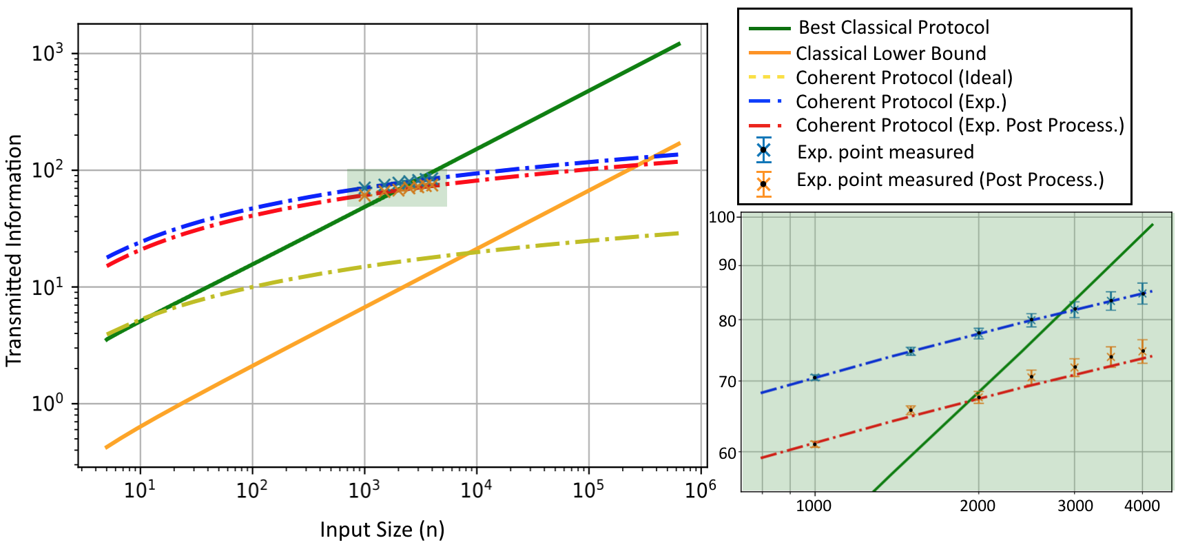
The quantum protocol with coherent state fingerprints for Sampling Matching that we introduced above has a complexity of for the transmitted information, where is the total mean photon number in the coherent fingerprint of Alice and is independent of . Note again that the exponential advantage concerns the information but not the communication resource. As before, for a fixed error probability , we calculate the optimal and the transmitted information for the quantum protocols with coherent states for the ideal, practical and post-selected cases. The latter here refers to the case where Bob outputs a parity outcome only when he obtains at least two single clicks in the experimental run. The results are shown in Fig. 8 (main panel), where we have also included the bounds for the best classical protocol and the classical lower bound. We remark that the threshold input size for observing a quantum advantage in the transmitted information with respect to the classical bounds is similar to Hidden Matching. However, as we will see below, Sampling Matching allows by its conception to reach this threshold in practice.
Experimental implementation. The experimental setup realizing in practice the schematic illustration of Fig. 6 and that we use for our proof-of-principle implementation of the Sampling Matching problem is shown in Fig. 7.
The coherent light is generated using a low line-width (10 kHz) continuous wave laser source operating at telecommunication wavelength (Laser1, Pure Photonics, nm). An amplitude modulator (AM) is then used to produce a sequence of coherent pulses with a 1-MHz repetition rate and pulse duration of 16 ns. A balanced 50:50 beam splitter (BS1) is used to monitor the power of the laser pulse, and we use a variable optical attenuator (VOA) to attenuate the pulses to the desired mean photon number. A second 50:50 beam splitter (BS2) splits the coherent pulses in two paths, sent to Alice and Bob. We introduce a delay line (DL, Kylia) to fine tune the path lengths of Alice and Bob, hence ensuring that their pulses arrive simultaneously at the 50:50 beam splitter BS3 and interfere optimally. Before this, Alice and Bob modulate their pulses, each using a phase modulator (PM). These are driven by a data acquisition card that provides the desired voltage levels, which is fixed for Bob and corresponding to her input for Alice. After interfering, the pulses are detected by telecom wavelength, free running InGaAs single-photon detectors and (ID230, IDQuantique). The detection events are recorded and analyzed with a precision of 1 ps using a time tagger (quTAG, QuTools).
The remaining components in the experimental setup are used for the phase correction loop that we use to monitor and correct the phase drift between Alice’s and Bob’s pulses. More specifically, we introduce a second continuous wave laser source (Laser2, Pure Photonics, nm) that is modulated similarly as described before. The pulses are directed through a circulator (C2) to BS3, where they are separated and then interfere on BS2 before being detected using a photodiode (PD). A second circulator (C1) prevents any of this light to go into the direction of Laser1. Furthermore, an optical filter (OF) is used in the path leading to detector to ensure that only light from Laser1 ( nm) reaches the detector. The difference in the length of the paths leading to and due to the presence of these components is appropriately compensated using a fiber before detector . To correct the phase drift, we use an averaging technique that estimates the phase drift over a block of pulses and corrects accordingly the phase in the next block (see Methods for details).
| 1000 | 1500 | 2000 | 2500 | 3000 | 3500 | 4000 | |
| 0.1 | 0.1 | 0.1 | 0.1 | 0.1 | 0.1 | 0.1 | |
| () | |||||||
| Runs | 848 | 568 | 475 | 381 | 317 | 272 | 238 |
| 115 | 68 | 62 | 45 | 38 | 31 | 28 | |
| 26 | 26 | 20 | 17 | 16 | 7 | 11 | |
| 0.03 | 0.04 | 0.04 | 0.04 | 0.05 | 0.03 | 0.05 | |
| () |
We are now ready to analyze the performance of our experiment for Sampling Matching. The relevant experimental parameters that have also been used for the previous simulations are shown in Table 1. The channel transmission loss, i.e., the loss from when Alice and Bob apply their phase modulation to the input of detectors and is 3.5 dB, hence . Furthermore, our single-photon detectors feature a quantum efficiency . As we have seen previously, the effect of these losses is that it is necessary to increase the mean photon number in the coherent fingerprint state compared to the ideal setting, in order to achieve the desired error rate .
The limited visibility, , is due to the imperfect interference of Alice and Bob’s pulses. It is important to remark that in our proof-of-principle implementation, we use a single laser for generating the pulses that Alice and Bob need to prepare their states, which is important for improving the visibility. However, the preparation of these states and all subsequent steps are done independently following the protocol, hence enabling us to use this setup for assessing the quantum advantage. As noted before, to achieve a high visibility, we also fine tune the delay line in the setup by following a simple calibration procedure whereby we send first sequences of inputs to both Alice and Bob and then sequences of and inputs to Alice and Bob, respectively, and observe the resulting detector clicks.
Finally, we further investigate the dark counts to make sure it is safe to neglect them in our analysis and indeed we observe that the signal click probability is substantially (three orders of magnitude) larger than the dark count probability. We also note that our detectors feature a dead time of 10 s, which means that after a detection event, the detector becomes idle for the next 10 pulses. For the input size targeted in our work (), the probability of a click within these pulses is extremely low due to the extremely low photon number of pulse that we use. This effect can therefore be safely neglected.
Based on these experimental parameters obtained in our setup, we estimate the optimal mean photon number for the entire coherent fingerprint state that achieves the desired error rate , and hence the mean photon number per pulse, , for input size around the threshold regions observed in Fig. 8, in particular from 1000 to 4000. These values are summarized in Table 2. In Fig. 8 (main and side panels), we show the experimentally obtained results for the transmitted information based on the above analysis. We see that for input size above 3000, our experiment for Sampling Matching provides an advantage in information compared to the best classical protocol, even within the error bars.
Furthermore, we also consider the case when Bob runs the Sampling Matching protocol multiple times (Runs in Table 2) and gives an output only for those runs where he gets a parity outcome. Without this post selection, every time Bob would not obtain the parity outcome, he would output a random parity with error rate . However, with post selection, since he rejects those no-parity outcome cases, he can succeed with a lower error rate . This can also be interpreted as performing the protocol with lower mean photon number,
| (24) |
The corresponding experimental values are provided in Table 2. In Fig. 8, we also plot the experimental results for the transmitted information in the post-selected scenario. We observe that the quantum protocol performs the Sampling Matching task with lower resources than the best classical protocol from input size of and above, hence demonstrating a quantum advantage in this case as well.
Discussion
The results that we have presented demonstrate rigorously a quantum advantage in the information resource in the one-way model of communication complexity. We achieved this by introducing the Sampling Matching problem, which is inspired by the emblematic Hidden Matching problem, and by analyzing it using the recently formulated coherent state mapping for quantum communication protocols. These two advancements enabled us to bypass the great challenge associated to the implementation of such tasks with the usual high dimensional multi-qubit fingerprint states.
As we have noted, an essential element of our proof-of-principle implementation is the ability to achieve high interference visibility, which has been facilitated in our case by the use of a single laser for generating the coherent states used by Alice and Bob for their sequences and the fine tuning of the path length difference using a delay line. In a full-scale implementation, where two separate lasers would be used, maintaining a good interference would require the use of stable, ultra narrow line-width lasers such that the phase difference between the pulses would be slower than the duration of the experimental run Comandar et al. 2016. In combination with phase correction techniques like the one used in our experiment, such an experiment is foreseeable in the near future and would be useful more generally for quantum communication tasks.
We also remark that our experimental results allow outperforming the best known classical protocol but not the classical lower bound. For this, we need an input size on the order of , which in turn would require attenuating the coherent pulses to a mean photon number per pulse of the same order. In this case, the dark counts of the single-photon detectors cannot be neglected any longer; indeed, the dark count rate exhibited by the detectors used in our experiment is precisely of this order and therefore it is impossible to show an advantage due to the noise. However, this would become possible using ultra low dark count superconducting nanowire single-photon detectors Schweickert et al. 2018, which also feature good quantum efficiencies and are commercially available.
The Sampling Matching problem that we have defined can also be seen as a verification tool, with applications in cryptographic and computational settings, most notably quantum money schemes, where it can replace the verification techniques that use Hidden Matching Gavinsky 2012; Amiri and Arrazola 2017. The soundness of verification in these schemes depends on the size of the input, hence since Sampling Matching allows for a simple implementation for large input sizes, our approach may readily increase the robustness of these schemes.
Methods
Phase correction procedure.
We apply an averaging technique over blocks of pulses to correct for the phase drift occurring between Alice’s and Bob’s pulse sequences. Such an averaging corresponds well to our conditions, with the relatively high -MHz repetition rate of our experiment and the high stability of our setup. We make blocks of pulses and track the average of the phase drift in one block to use it to correct the drift of the subsequent block. The block construction we use is detailed in Fig. 9. We choose a block size of 8192 pulses. The first 7680 pulses are used for protocol run. The second segment of the block, , tracks the phase drift in the path corresponding to Alice’s PM. This is done by providing a ramp voltage in Alice’s PM from -5V to +5V, and 0V in Bob’s PM across 256 pulses. The response of the linear ramp voltage across a phase modulator is a cosine function which is tracked using the photodiode PD. We then model the expected response corresponding to the actual response, hence obtaining the information on the phase and the phase drift up to a certain error. If is the voltage corresponding to the phase drift, then we add this factor to the voltage provided to Alice’s PM for the next block, i.e., . We similarly track and correct the phase drift in Bob’s PM over the last 256 pulses of the block, .

Acknowledgments
We thank Frédéric Grosshans, Nobert Lütkenhaus, Luis Trigo Vidarte, and Adeline Orieux, for useful discussions. This research was supported by the European Research Council projects QCC (I.K.) and QUSCO (E.D.), the French National Research Agency project quBIC and the BPI France project RISQ.
References
- Harrow and Montanaro (2017) A. W. Harrow and A. Montanaro, Nature 549, 203 (2017).
- Aaronson and Arkhipov (2011) S. Aaronson and A. Arkhipov, in Proceedings of the forty-third annual ACM symposium on Theory of computing (ACM, 2011), pp. 333–342.
- Neville et al. (2017) A. Neville, C. Sparrow, R. Clifford, E. Johnston, P. M. Birchall, A. Montanaro, and A. Laing, Nat. Phys. 13, 1153 (2017).
- Broome et al. (2013) M. A. Broome, A. Fedrizzi, S. Rahimi-Keshari, J. Dove, S. Aaronson, T. C. Ralph, and A. G. White, Science 339, 794 (2013).
- Tillmann et al. (2013) M. Tillmann, B. Dakić, R. Heilmann, S. Nolte, A. Szameit, and P. Walther, Nature Photon. 7, 540 (2013).
- Crespi et al. (2013) A. Crespi, R. Osellame, R. Ramponi, D. J. Brod, E. F. Galvão, N. Spagnolo, C. Vitelli, E. Maiorino, P. Mataloni, and F. Sciarrino, Nature Photon. 7, 545 (2013).
- Spagnolo et al. (2014) N. Spagnolo, C. Vitelli, M. Bentivegna, D. J. Brod, A. Crespi, F. Flamini, S. Giacomini, G. Milani, R. Ramponi, P. Mataloni, et al., Nature Photon. 8, 615 (2014).
- Farhi and Harrow (2016) E. Farhi and A. W. Harrow, arXiv preprint arXiv:1602.07674 (2016).
- Bremner et al. (2017) M. J. Bremner, A. Montanaro, and D. J. Shepherd, Quantum 1, 8 (2017).
- Bravyi et al. (2017) S. Bravyi, D. Gosset, and R. Koenig, arXiv preprint arXiv:1704.00690 (2017).
- Gao et al. (2017) X. Gao, S.-T. Wang, and L.-M. Duan, Physical review letters 118, 040502 (2017).
- Bermejo-Vega et al. (2018) J. Bermejo-Vega, D. Hangleiter, M. Schwarz, R. Raussendorf, and J. Eisert, Physical Review X 8, 021010 (2018).
- Aaronson and Chen (2016) S. Aaronson and L. Chen, arXiv preprint arXiv:1612.05903 (2016).
- Boixo et al. (2018) S. Boixo, S. V. Isakov, V. N. Smelyanskiy, R. Babbush, N. Ding, Z. Jiang, M. J. Bremner, J. M. Martinis, and H. Neven, Nature Physics 14, 595 (2018).
- Aaronson et al. (2008) S. Aaronson, S. Beigi, A. Drucker, B. Fefferman, and P. Shor, in Computational Complexity, 2008. CCC’08. 23rd Annual IEEE Conference on (IEEE, 2008), pp. 223–236.
- Arrazola et al. (2018) J. M. Arrazola, E. Diamanti, and I. Kerenidis, npj Quantum Information 4, 56 (2018).
- Scarani et al. (2009) V. Scarani, H. Bechmann-Pasquinucci, N. J. Cerf, M. Dušek, N. Lütkenhaus, and M. Peev, Rev. Mod. Phys. 81, 1301 (2009).
- Diamanti et al. (2016) E. Diamanti, H.-K. Lo, B. Qi, and Z. Yuan, npj Quantum Information 2, 16025 (2016).
- Donaldson et al. (2016) R. J. Donaldson, R. J. Collins, K. Kleczkowska, R. Amiri, P. Wallden, V. Dunjko, J. Jeffers, E. Andersson, and G. S. Buller, Phys. Rev. A. 93, 012329 (2016).
- Pappa et al. (2014) A. Pappa, P. Jouguet, T. Lawson, A. Chailloux, M. Legré, P. Trinkler, I. Kerenidis, and E. Diamanti, Nature Commun. 5, 3717 (2014).
- Barz et al. (2012) S. Barz, E. Kashefi, A. Broadbent, J. F. Fitzsimons, A. Zeilinger, and P. Walther, Science 335, 303 (2012).
- McCutcheon et al. (2016) W. McCutcheon, A. Pappa, B. A. Bell, A. McMillan, A. Chailloux, T. Lawson, M. Mafu, D. Markham, E. Diamanti, I. Kerenidis, et al., Nat. Commun. 7, 13251 (2016).
- Hensen et al. (2015) B. Hensen, H. Bernien, A. Dréau, A. Reiserer, N. Kalb, M. Blok, J. Ruitenberg, R. Vermeulen, R. Schouten, C. Abellán, et al., Nature 526, 682 (2015).
- Pappa et al. (2015) A. Pappa, N. Kumar, T. Lawson, M. Santha, S. Zhang, E. Diamanti, and I. Kerenidis, Phys. Rev. Lett. 114, 020401 (2015).
- Buhrman et al. (2001) H. Buhrman, R. Cleve, J. Watrous, and R. De Wolf, Phys. Rev. Lett. 87, 167902 (2001).
- Buhrman et al. (1998) H. Buhrman, R. Cleve, and A. Wigderson, in Proceedings of the thirtieth annual ACM symposium on Theory of computing (1998), pp. 63–68.
- Raz (1999) R. Raz, in Proceedings of the thirty-first annual ACM symposium on Theory of computing (1999), pp. 358–367.
- Gavinsky et al. (2007) D. Gavinsky, J. Kempe, I. Kerenidis, R. Raz, and R. De Wolf, in Proceedings of the thirty-ninth annual ACM symposium on Theory of computing (2007), pp. 516–525.
- Gavinsky (2016) D. Gavinsky, arXiv preprint arXiv:1602.05059 (2016).
- Regev and Klartag (2011) O. Regev and B. Klartag, in Proceedings of the forty-third annual ACM symposium on Theory of computing (2011), pp. 31–40.
- Bar-Yossef et al. (2004) Z. Bar-Yossef, T. S. Jayram, and I. Kerenidis, in Proceedings of the thirty-sixth annual ACM symposium on Theory of computing (ACM, 2004), pp. 128–137.
- Arrazola and Lütkenhaus (2014a) J. M. Arrazola and N. Lütkenhaus, Phys. Rev. A 90, 042335 (2014a).
- Arrazola and Lütkenhaus (2014b) J. M. Arrazola and N. Lütkenhaus, Phys. Rev. A 89, 062305 (2014b).
- Xu et al. (2015) F. Xu, J. M. Arrazola, K. Wei, W. Wang, P. Palacios-Avila, C. Feng, S. Sajeed, N. Lütkenhaus, and H.-K. Lo, Nature Commun. 6, 8735 (2015).
- Guan et al. (2016) J.-Y. Guan, F. Xu, H.-L. Yin, Y. Li, W.-J. Zhang, S.-J. Chen, X.-Y. Yang, L. Li, L.-X. You, T.-Y. Chen, et al., Phys. Rev. Lett. 116, 240502 (2016).
- Kumar et al. (2017) N. Kumar, E. Diamanti, and I. Kerenidis, Physical Review A 95, 032337 (2017).
- Wei et al. (2018) K. Wei, N. Tischler, S.-R. Zhao, Y.-H. Li, J. M. Arrazola, Y. Liu, W. Zhang, H. Li, L. You, Z. Wang, et al., arXiv preprint arXiv:1810.10238 (2018).
- Sasaki et al. (2014) T. Sasaki, Y. Yamamoto, and M. Koashi, Nature 509, 475 (2014).
- Guan et al. (2015) J.-Y. Guan, Z. Cao, Y. Liu, G.-L. Shen-Tu, J. S. Pelc, M. M. Fejer, C.-Z. Peng, X. Ma, Q. Zhang, and J.-W. Pan, Phys. Rev. Lett. 114, 180502 (2015).
- Buhrman et al. (2011) H. Buhrman, O. Regev, G. Scarpa, and R. De Wolf, in Computational Complexity (CCC), 2011 IEEE 26th Annual Conference on (IEEE, 2011), pp. 157–166.
- Kahn et al. (1988) J. Kahn, G. Kalai, and N. Linial, The influence of variables on Boolean functions (IEEE, 1988).
- Comandar et al. (2016) L. Comandar, M. Lucamarini, B. Fröhlich, J. Dynes, A. Sharpe, S.-B. Tam, Z. Yuan, R. V. Penty, and A. Shields, Nature Photonics 10, 312 (2016).
- Schweickert et al. (2018) L. Schweickert, K. D. Jöns, K. D. Zeuner, S. F. Covre da Silva, H. Huang, T. Lettner, M. Reindl, J. Zichi, R. Trotta, A. Rastelli, et al., Applied Physics Letters 112, 093106 (2018).
- Gavinsky (2012) D. Gavinsky, in Computational Complexity (CCC), 2012 IEEE 27th Annual Conference on (IEEE, 2012), pp. 42–52.
- Amiri and Arrazola (2017) R. Amiri and J. M. Arrazola, Physical Review A 95, 062334 (2017).