Excited Kerr black holes with scalar hair
Abstract
In the context of complex scalar field coupled to Einstein gravity theory, we present a novel family of solutions of Kerr black holes with excited-state scalar hair inspired by the work of Herdeiro and Radu in [Phys. Rev. Lett. 112, 221101 (2014)], which can be regarded as numerical solutions of rotating compact objects with excited scalar hair, including boson stars and black holes. In contrast to Kerr black holes with ground state scalar hair, we find that the first-excited Kerr black holes with scalar hair have two types of nodes, including radial and angular nodes. Moreover, in the case of radial nodes the curves of the mass versus the frequency form nontrivial loops, and in the case of angular nodes the curves can be divided into two kinds: closed and open loops. We also study the dependence of the horizon area on angular momentum and Hawking temperature.
I Introduction
One of the most interesting discoveries in the study of black holes (BHs) is uniqueness theorem Chrusciel:2012jk, which states that the four-dimensional, asymptotically flat black hole solutions of the Einstein field equations is Kerr-Newman black hole (BH). The theorem is only valid for the Einstein-Maxwell theory, however, when more general types of matter fields are coupled to gravity, a few counterexamples to uniqueness theorem have been found during the last few years. For instance, the first example of black hole with non-Abelian hair was discovered in four-dimensional Einstein-Yang-Mills theory Colored1; Colored2. Soon after that, the black holes with Skyrme hair were found in the non-linear sigma-model of Skyrme coupled to gravity Droz:1991cx and with Yang-Mills-Dilaton hair in Einstein Yang-Mills-Dilaton theory H1.
Recently, a family of Kerr black holes with scalar hair (KBHsSH) were discovered by Herdeiro and Radu in the four-dimensional Einstein gravity coupled to a complex scalar field Herdeiro:2014goa. The scalar hair is a free massive field, moreover, it takes a time-dependent harmonic value in which the time variation is sinusoidal and the frequency of the complex field needs to obey the synchronisation condition
| (1) |
where the constant is the horizon angular velocity and is the azimuthal harmonic index. The solutions of Kerr black holes with scalar hair can reduce to spinning boson stars (BSs) in the limit of vanishing horizon area. The stability of Kerr black holes with scalar hair was discussed in Refs. Ganchev:2017uuo; Degollado:2018ypf and the bound scalar hair can be regarded as the zero mode of the superradiant instability Hod:2012px; Benone:2014ssa. In Refs. Herdeiro:2014jaa; Cunha:2015yba, the properties of ergosurfaces and shadows were also investigated. Furthermore, the study of hairy black holes can be extended to the Proca hair case Herdeiro:2016tmi, Kerr-Newman BH Delgado:2016jxq, non-minimal coupling case Herdeiro:2018wvd, and spinning BHs with Skyrme hair Herdeiro:2018daq. Especially, considering the model of gravity coupled to self-interacting scalar field Herdeiro:2015tia; Herdeiro:2016gxs, one can obtain the solution of Kerr black holes with ultra-light scalar hair. The study of relevant astrophysical observational signatures of Kerr black holes with scalar hair has been investigated in Refs. Ni:2016rhz; Cao:2016zbh; Shen:2016acv; Zhou:2017glv. With the study on long-term numerical evolutions of the superradiant instability of Kerr black hole by East and Pretorius East:2017ovw, the relationship between formation properties of Kerr black hole with Proca hair and superradiant instability of Kerr black hole was discussed in Refs. Herdeiro:2017phl; East:2018glu. Besides, a variety of analytical studies on hairy black holes have been undertaken in Refs. Hod:2013zza; Hod:2014baa; Hod:2017kpt; Hod:2016yxg; Hod:2017rmh; Hod:2016lgi; Brihaye:2018woc, and there have been a lot of attention to study hairy black holes recently Brihaye:2016vkv; Herdeiro:2015moa; Brito:2015pxa; Herdeiro:2017oyt; Herdeiro:2017fhv; Herdeiro:2017fhv; Delgado:2018khf. See Ref. Herdeiro:2015gia for a detailed discussion of numerical method and Ref. Herdeiro:2015waa for a review.
Until now, only Kerr black holes with the scalar hair in the ground state have been considered, that is, the scalar hair can keep sign along the radial direction. On the other hand, in the astrophysical applications of boson stars Schunck:1997FE; Yoshida:1997qf; Schunck:1996he, the authors of Refs. Bernal:2009zy; Collodel:2017biu found some boson star solutions with excited scalar field which were beneficial to obtain more realistic rotation curves of spiral galaxies. So, it will be interesting to see whether there are solutions of Kerr black hole with excited-state scalar hair in Einstein-Klein-Gordon theory. In the present paper, we would like to numerically solve the system of field equations and give a family of Kerr black holes with first-excited state scalar hair, which can be divided into two categories of radial nodes and angular nodes .
The paper is organized as follows. In Sect. II, we introduce the model of the four-dimensional Einstein gravity coupled to a free, complex scalar field and adopt the same axisymmetric metric with Kerr-like coordinates as the ansatz in Ref. Herdeiro:2014goa. In Sect. III, the boundary conditions of excited Kerr black holes with scalar hair and rotating boson stars are studied. We show the numerical results of the equations of motion and study the characteristics of radial nodes and angular nodes in Sect. V. The conclusion and discussion are given in the last section.
II The model setup
Let us begin with the model of (3+1)-dimensional Einstein gravity coupled to a free, complex massive scalar field, with the Lagrangian density
| (2) |
where is the gravitational constant and the term proportional to is known as a mass term. The equations of motion of the scalar field are given by
| (3) |
and Einstein field equations read as
| (4) |
Note that if the complex, massive scalar field vanishes, the solution of Einstein equations (4), which can describe the stationary axisymmetric asymptotically flat black hole with mass and angular momentum, is the well-known Kerr black hole. In terms of Boyer-Lindquist coordinates, the Kerr metric reads
| (5) | |||||
with and the Kerr horizon function . Here, the constants and are the angular momentum per unit mass and the mass of the Kerr BH as measured from the infinite boundary, respectively. The non-extremal Kerr black hole has the event horizon and the Cauchy horizon at
| (6) |
The Hawking temperature and angular velocity of the Kerr black hole are given by
| (7) |
When there exists a non-trivial configuration of the complex scalar field, Herdeiro and Radu constructed a class of Kerr BH solutions with ground state scalar hair Herdeiro:2014goa. In order to construct stationary solutions of a Kerr BH with excited state scalar hair, we also adopt the axisymmetric metric with Kerr-like coordinates Herdeiro:2014goa; Herdeiro:2015gia within the following ansatz
| (8) |
with and the constant is related to event horizon radius. In addition, the ansatz of the complex matter field is given by
| (9) |
Here, is the azimuthal angle and the five functions , and depend on the radial distance and polar angle . The constant is the frequency of the complex scalar field and is the azimuthal harmonic index. Subscript is named as the principal quantum number of the scalar field, and is regarded as the ground state and as the excited states.
By demanding the Euclidean space smooth and continuous at the horizon, one can determine the Hawking temperature with the metric (8)
| (10) |
The Bekenstein-Hawking entropy associated with the horizon is given by
| (11) |
The field equations (3) and (4) with the ansatzs (8) and (9) are a set of seven non-linear coupled partial differential equations (PDEs). One of the seven equations which comes from the scalar field equation (3) is a second-order PDE for the function . With linear combinations of the components of Einstein field equations, the remaining six equations from Eq. (4) yield a new set of PDEs, including four equations for finding solutions and two constraint equations for checking the numerical accuracy. It is not convenient to write down these seven equations in this paper, and see Ref. Herdeiro:2015gia for more details. With numerical methods for solving these equations of motion, we could obtain two classes of solutions: horizonless boson star (BS) solutions with and hairy black hole solutions with . The Solitonic solutions can be seen as deformations of the global Minkowski spacetime, while the hairy black hole solutions closely correspond to deformations of the Kerr BH.
It is well known that the ground state scalar hair has no node, that is, along the radial direction, the value of the scalar field has the same sign. When studying Kerr black holes with the excited scalar hair, we find that there are two types of nodes, including radial and angular nodes. Radial nodes are the points where the value of the scalar field can change sign along the radial direction, while, angular nodes are the points where the value of the scalar field can change sign along the angular direction.
III Boundary conditions
Before numerically solving the differential equations instead of seeking the analytical solutions, we should obtain the asymptotic behaviors of the five functions , and , which is equivalent to give the boundary conditions we need. Considering the properties of Kerr black holes with excited state scalar hair, we will still use the boundary conditions by following the same steps as the ground state given in Refs. Herdeiro:2014goa; Herdeiro:2015gia.
Considering an axial symmetry system, we have polar angle reflection symmetry on the equatorial plane, and thus it is convenient to consider the coordinate range . So, we require the functions to satisfy the following boundary conditions at
| (12) |
and set axis boundary conditions at where regularity must be imposed Dirichlet boundary conditions on and Neumann boundary conditions on the other functions
| (13) |
In addition, the asymptotic behaviors near the boundary are
| (14) |
And finally, by expanding the equations of motion near as a power series in , we have
| (15) |
and
| (16) |
for black hole solutions with , and
| (17) |
for boson star solutions with . Note that the values of and are the constants independent of the polar angle .
Properties of the black hole can be obtained from the asymptotic behavior of the solutions. Near the boundary , the metric functions and have the following forms
| (18) |
where the parameters and are the mass and angular momentum of the hairy Kerr black hole, respectively.
IV Numerical results
In this section, we will solve the above coupled equations (3) and (4) with the ansatzs (8) and (9) numerically. It is convenient to introduce a new coordinate which can compactify the radial coordinate and implies that at and at . Thus the inner and outer boundaries of the shell are fixed at and , respectively. After solving the equations numerically, we can study the dependence on the frequency , the scalar field mass and event horizon , respectively. Due to scalar invariance, we can work at a fixed scalar field mass. Moreover, for simplicity, we choose .
Next, we will discuss the principal quantum number of the Kerr BH with scalar hair, which is the case of the first-excited state, and show two classes of radial and angular node solutions, respectively. The numerical data files for the sample of reference solutions for excited Kerr BHs with scalar hair are included in an ancillary file.
IV.1 Radial nodes
Along the angular direction, the value of the scalar field has the same sign for the case of radial node . However, along the radial direction, the scalar field changes sign once at some point which is called radial node. So, we name this case as the first bound excited state with radial node, signed with . In the following, we will show the results of excited boson star and Kerr BH with scalar hair, respectively.
IV.1.1 Boson star


Firstly, as an example, we show in Fig. 1 two typical results of our numerical program for the scalar field as a function of and with for the same parameter . Along the equatorial plane at , we can observe that the scalar field changes sign once from the center of the boson star to the boundary in a node where there is zero value. In both graphs the function has even parity and could keep the same sign for the angular variable . In the left panel of Fig. 1, the distribution of the scalar field is near the boundary of spacetime, while the right panel shows the distribution is near the center of the boson star. Though both plots have the same parameter, the first graph belongs to a branch of solutions with higher black hole mass , and the second graph belongs to a second set of unstable solutions with lower black hole mass. These behaviors are further shown in Fig. 2.
To study the properties of the rotating excited state boson star, in the left panel of Fig. 2 we exhibit the mass versus the frequency for three sets of boson stars with the azimuthal harmonic index , represented by the black, red and blue lines, respectively, and plot the mass as a function of the angular momentum for the corresponding values of in the right panel of Fig. 2. Note that in this paper all physical quantities are expressed in units set by . We can see from the left plot that there exist excited state boson stars for , which means the excited state solutions are still bound states and similar to the ground state boson star in Ref. [15]. The spiral curve with starts from the vacuum and revolves into a central region of the graph. Moreover, when the curve spirals into the center, the numerical error begins to increase and a finer mesh is required to calculate. For simplify, we only show the part of the curve for , which have similar behaviour as that of . Comparing with the ground BS curve in Ref. Herdeiro:2014goa, we can see that the mass of the excited BS is more heavier than that of the ground state, and the minimum value of of the excited state is larger than that of the ground state.
On the right panel of Fig. 2, we show how the BS mass varies as a function of the angular momentum with different azimuthal harmonic index (black lines), 2 (red lines), and 3 (green lines). These three zigzag patterns are exactly similar to that for the ground state in Ref. Herdeiro:2014goa, where the inset shows the detail of the zigzag curves with .
IV.1.2 Black hole
In order to obtain the excited Kerr black hole with scalar hair, we require the conditon . In the left panel of Fig. 3, we plot the mass of the excited KBHsSH as a function of the frequency with . The black line represents the excited BS curve which has been discussed in Fig. 2. We plot three curves with the event horizon (the green lines ), (the red lines), and (the blue lines), respectively, and the domain of existence of Kerr BHs is indicated by the orange shaded area.
With the decrease of the frequency , the mass of the excited KBHsSH increases firstly and then it reaches a maximum point. Further decreasing , the mass begins to decrease until a minimum value of below which no excited KBHsSHs are found. As the frequency continues to increase to a maximum value, we obtain a second set of solutions with lower mass. It is interesting that the curve does not form a spiral. Instead, they form a closed loop. As the value of the radius decreases to zero, the curve of the excited Kerr BH with scalar hair star is very close to the boson star curve. Here, we only exhibit in Fig. 3 the solution of the mode, and the other values of have similar behaviour. In the right panel of Fig. 3, we show the mass as a function of the angular momentum for . We find that the multi-zigzag pattern is more complex than that of the ground case, and more details are shown in the inset.
As typical examples for our numerical results, we show in Fig. 4 the area of the event horizon as functions of the angular momentum and temperature , respectively, by taking (black), 0.05 (red), and 0.1 (green). In the left panel we can see that the black hole solution with a fixed radius has the maximal angular momentum and there are no hairy black hole solutions for . There exist two curve branches of which the area of the event horizon has different behaviors with . With the decreasing of , the area of one branch decreases and the other increases. Moreover, for the large area branch, when the size of decreases, one obtains a new third set of branch in which the area of the hairy BH is an increasing function of . The large area branch of the hairy BH is no longer a monotone function of . Indeed, this behavior is in good agreement with the numerical results in Fig. 3. More details are given in the inset plotted in the left panel of Fig. 4. In the right panel of Fig. 4, we can see that for a fixed temperature , the area increases with . Moreover, when the event horizon of the hairy black hole decreases, the temperature can have a wider range. As an example in Fig.4, we show the range of the temperature , which is between 0.077 and 0.18 for the pink line with radius .
IV.2 Angular nodes
In the last subsection, we gave a family of boson star and hairy black hole solutions with the excited state, which means the value of the scalar field has the same sign along the angular direction. Next, we will show other numerical results in which the value of the scalar field can change the sign along the angular direction. In addition, along the radial direction, the scalar field can keep sign or only change sign once at some radial nodes, which still belongs to the first bound excited state. So, we denote this family of solutions with .
IV.2.1 Boson star
To describe the properties of the first bound excited state, we show the spatial profile of three typical numerical results for the scalar field with in Fig. 5. These three plots have the same angular momentum . The sign of the scalar field could change along the angular direction. However, along the radial direction, the scalar field changes sign in the bottom left panel or keeps sign in the top panel. These three plots correspond to three branches of boson star solutions, respectively. As an example, the distribution of the scalar field as a function of the coordinate for different values of the angular momentum in the equatorial plane at is shown in the bottom right panel of Fig. 5.


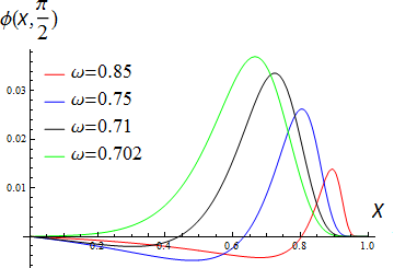
After obtaining the numerical solution of rotating excited state boson stars, in the left panel of Fig. 6 we show the mass as a function of the frequency with the azimuthal harmonic index (black line), 2 (red line), 3 (blue line), respectively, and plot the mass as a function of the angular momentum for the corresponding values of in the right panel of Fig. 6. From the graphics, it is obvious that there exists excited state boson star for and the excited state solution is still bound state.
In diagram, the fitting curve emanating from the point (, ) moves away as it revolves around a central region of the diagram. In contrast to the ground boson stars in Ref. Herdeiro:2014goa and the excited boson stars with , the excited sets of solutions with do not exhibit a spiraling behavior. For example, for , we can see that with the decrease of the frequency , the mass of boson stars begins to increase and then decrease until a minimum value of . Further, below the minimum value we obtain a second branch of excited boson stars with lower mass. So far these data show a similar behavior as the ground state. However, above the minimum value of we obtain a third set of unstable solutions with larger mass, where the curve does not spiral into the center. It is noted that in contrast to the behavior of the curve in the left panel of Fig. 2, we see that the mass of the excited solutions with is more heavier than the case of , while the minimum value of of the excited state with is smaller than the case of .
We exhibit in the right panel of Fig. 6 how the BS mass varies as a function of the angular momentum with the azimuthal harmonic index (black line), (red line), and (blue line), respectively. These three zigzag patterns are similar to the case of in the right panel of Fig. 2, and in the inset we show the detail of the zigzag curve with .
IV.2.2 Black hole
Let us now study the physical properties of rotating excited hairy black hole solutions with . In the left panel of Fig. 7, we show the BH mass as a function of the frequency with several radii of event horizon in mode. In the graph, the curve of the black colour represents the excited boson star with , and the solution domain of Kerr BHs is indicated by the orange shaded area. It is interesting to note that these families of excited hairy black hole solutions with do not present the spiraling behavior as that of in the left panel of Fig. 3. According to the dependence of mass on the angular momentum, the curves can be divided into two kinds as follows:
- 1.
Closed loop: For and 0.07, the curves of the radially excited KBHsSH originally start from the maximal frequency at the Kerr BH vacuum, and then reach a minimal frequency. Further increasing , the mass begins to decrease until a new maximum value of and then the curves turn round to another minimal frequency, and finally end at the maximal frequency at the vacuum solution. So, the set of curves form a closed loop which is similar to the excited KBHsSH curve in the left panel of Fig. 3.
- 2.
Open loop: For the small value of the event horizon ( the pink line), the curve is not continuous and has a break point. The similar behaviour also occurs for the curves with , and . Note that, in order to avoid overlapping with the black curve of boson star, we only show the part of these curves.
The above two kinds of solutions with are very different from that of the ground state. In the left panel, we only exhibit the solution of the lowest modes, and the higher values of also have similar properties. Furthermore, in the right panel of Fig. 7, we plot the mass as a function of the angular momentum for . We can see the zigzag pattern also has a break point, which just corresponds to the position in the curve, and more details are shown in the inset.
The relation between the event horizon and angular momentum is shown in the left panel of in Fig. 8, where we plot several typical examples for our numerical results by taking and 0.1, respectively. We find that hairy black hole solutions with and 0.1 have similar behavior as those given in the left panel of Fig. 4. However, the black curve with is not continuous and has a break point. There exist two separate branches of how the area of the event horizon varies with . Indeed, this behavior is in good agreement with the numerical results in Fig. 7. More details are shown as an inset plot in the left panel of Fig. 8. In the right panel, the event horizon as a function of the temperature is shown by taking and 0.1, respectively. The curves with and 0.1 are continuum, while the ones with and 0.05 have a break point. Moreover, with decreasing , the range of break becomes larger.
V Conclusion
In this paper, we have analyzed the model of (3+1)-dimensional Einstein gravity coupled to a complex, massive scalar field and numerically constructed the solutions of rotating compact objects with excited scalar hair, including boson stars and black holes. Comparing with the ground state solution in Ref. Herdeiro:2014goa, we found that the first-excited Kerr BHs with scalar hair have two types of nodes, radial and angular nodes. In the former case the curves of the mass versus the frequency form nontrivial loops, starting from and ending at the trivial solution at . In the latter case the curves can be divided into two types: the closed and open loops. For a larger value of the event horizon radius, the curve forms a closed loop. While for a small one, the curve is not continuous and has a break point. In addition, the range of break point decreases with . It is notable that there is a similar situation in atomic theory and quantum mechanics, for example, the first excited state of hydrogen has an electron in the 2s-orbital or 2p-orbital, which corresponds to the radial or angel node, respectively. From the numerical results, we can see that the mass of the excited KBHsSH solution is heavier than the ground state. Moreover, the state with has higher mass level than the one with .
There are several interesting extensions of our work. First, we have studied the first excited Kerr BH with a free scalar hair, we would like to investigate how self-interactions of the scalar field affects the excited Kerr black holes with scalar hair inspired by the work Herdeiro:2015tia. The second extension of our study is to construct generalized multi-scalar hair configurations, where two coexisting states of the scalar field are presented, including ground and excited states. The first step in this direction was done in Bernal:2009zy, where the rotating boson star with coexisting ground and excited states was constructed. Finally, we are planning to study the model of the Einstein-complex-Proca model and construct the excited Kerr BHs with Proca hair in future work.
Acknowledgement
YQW would like to thank Hao Wei and Li Li for helpful discussion. Some computations were performed on the Shared Memory system at Institute of Computational Physics and Complex Systems in Lanzhou University. This work was supported by the Natural Science Foundation of China (Grants No. 11675064, No. 11522541 and No. 11875175), and the Fundamental Research Funds for the Central Universities (Grants No. lzujbky-2017-182, No. lzujbky2017-it69 and No. lzujbky-2018-k11).
References
- (1) P. T. Chrusciel, J. Lopes Costa and M. Heusler, “Stationary Black Holes: Uniqueness and Beyond,” Living Rev. Rel. 15, 7 (2012) [arXiv:1205.6112 [gr-qc]].
- (2) P. Bizo, “Colored black holes,” Phys. Rev. Lett 64, 2844 (1990).
- (3) M. S. Volkov and D. V. Gal’tsov, Sov. J. Nucl. Phys. 51, 1171 (1990).
- (4) S. Droz, M. Heusler and N. Straumann, “New black hole solutions with hair,” Phys. Lett. B 268, 371 (1991).
- (5) G. Lavrelashvili and D. Maison, “Regular and black hole solutions of Einstein Yang-Mills Dilaton theory,” Nucl. Phys. B 410, 407 (1993).
- (6) C. A. R. Herdeiro and E. Radu, “Kerr black holes with scalar hair,” Phys. Rev. Lett. 112, 221101 (2014) [arXiv:1403.2757 [gr-qc]].
- (7) B. Ganchev and J. E. Santos, “Scalar hairy black holes in four dimensions are unstable,” Phys. Rev. Lett. 120, no. 17, 171101 (2018) [arXiv:1711.08464 [gr-qc]].
- (8) J. C. Degollado, C. A. R. Herdeiro and E. Radu, “Effective stability against superradiance of Kerr black holes with synchronised hair,” Phys. Lett. B 781, 651 (2018) [arXiv:1802.07266 [gr-qc]].
- (9) S. Hod, “Stationary Scalar Clouds Around Rotating Black Holes,” Phys. Rev. D 86, 104026 (2012) Erratum: [Phys. Rev. D 86, 129902 (2012)] [arXiv:1211.3202 [gr-qc]].
- (10) C. L. Benone, L. C. B. Crispino, C. Herdeiro and E. Radu, “Kerr-Newman scalar clouds,” Phys. Rev. D 90, no. 10, 104024 (2014) [arXiv:1409.1593 [gr-qc]].
- (11) C. Herdeiro and E. Radu, “Ergosurfaces for Kerr black holes with scalar hair,” Phys. Rev. D 89, no. 12, 124018 (2014) [arXiv:1406.1225 [gr-qc]].
- (12) P. V. P. Cunha, C. A. R. Herdeiro, E. Radu and H. F. Runarsson, “Shadows of Kerr black holes with scalar hair,” Phys. Rev. Lett. 115, no. 21, 211102 (2015) [arXiv:1509.00021 [gr-qc]].
- (13) C. Herdeiro, E. Radu and H. Runarsson, “Kerr black holes with Proca hair,” Class. Quant. Grav. 33, no. 15, 154001 (2016) [arXiv:1603.02687 [gr-qc]].
- (14) J. F. M. Delgado, C. A. R. Herdeiro, E. Radu and H. Runarsson, “Kerr-Newman black holes with scalar hair,” Phys. Lett. B 761, 234 (2016) [arXiv:1608.00631 [gr-qc]].
- (15) C. A. R. Herdeiro and E. Radu, “Spinning boson stars and hairy black holes with nonminimal coupling,” Int. J. Mod. Phys. D 27, no. 11, 1843009 (2018) [arXiv:1803.08149 [gr-qc]].
- (16) C. Herdeiro, I. Perapechka, E. Radu and Y. Shnir, “Skyrmions around Kerr black holes and spinning BHs with Skyrme hair,” [arXiv:1808.05388 [gr-qc]].
- (17) C. A. R. Herdeiro, E. Radu and H. R��narsson, “Kerr black holes with self-interacting scalar hair: hairier but not heavier,” Phys. Rev. D 92, no. 8, 084059 (2015) [arXiv:1509.02923 [gr-qc]].
- (18) C. A. R. Herdeiro, E. Radu and H. F. R��narsson, “Spinning boson stars and Kerr black holes with scalar hair: the effect of self-interactions,” Int. J. Mod. Phys. D 25, no. 09, 1641014 (2016) [arXiv:1604.06202 [gr-qc]].
- (19) Y. Ni, M. Zhou, A. Cardenas-Avendano, C. Bambi, C. A. R. Herdeiro and E. Radu, “Iron K line of Kerr black holes with scalar hair,” JCAP 1607, no. 07, 049 (2016) [arXiv:1606.04654 [gr-qc]].
- (20) Z. Cao, A. Cardenas-Avendano, M. Zhou, C. Bambi, C. A. R. Herdeiro and E. Radu, “Iron K line of boson stars,” JCAP 1610, no. 10, 003 (2016) [arXiv:1609.00901 [gr-qc]].
- (21) T. Shen, M. Zhou, C. Bambi, C. A. R. Herdeiro and E. Radu, “Iron K line of Proca stars,” JCAP 1708, 014 (2017) [arXiv:1701.00192 [gr-qc]].
- (22) M. Zhou, C. Bambi, C. A. R. Herdeiro and E. Radu, “Iron K line of Kerr black holes with Proca hair,” Phys. Rev. D 95, no. 10, 104035 (2017) [arXiv:1703.06836 [gr-qc]].
- (23) W. E. East and F. Pretorius, “Superradiant Instability and Backreaction of Massive Vector Fields around Kerr Black Holes,” Phys. Rev. Lett. 119, no. 4, 041101 (2017) [arXiv:1704.04791 [gr-qc]].
- (24) W. E. East, “Massive Boson Superradiant Instability of Black Holes: Nonlinear Growth, Saturation, and Gravitational Radiation,” Phys. Rev. Lett. 121, 131104 (2018) [arXiv:1807.00043 [gr-qc]].
- (25) C. A. R. Herdeiro and E. Radu, “Dynamical Formation of Kerr Black Holes with Synchronized Hair: An Analytic Model,” Phys. Rev. Lett. 119, no. 26, 261101 (2017) [arXiv:1706.06597 [gr-qc]].
- (26) S. Hod, “Stationary resonances of rapidly-rotating Kerr black holes,” Eur. Phys. J. C 73, no. 4, 2378 (2013) [arXiv:1311.5298 [gr-qc]].
- (27) S. Hod, “Kerr-Newman black holes with stationary charged scalar clouds,” Phys. Rev. D 90, no. 2, 024051 (2014) [arXiv:1406.1179 [gr-qc]].
- (28) S. Hod, “Extremal Kerr-Newman black holes with extremely short charged scalar hair,” Phys. Lett. B 751, 177 (2015) [arXiv:1707.06246 [gr-qc]].
- (29) S. Hod, “The large-mass limit of cloudy black holes,” Class. Quant. Grav. 32, no. 13, 134002 (2015) [arXiv:1607.00003 [gr-qc]].
- (30) S. Hod, “A no-short scalar hair theorem for rotating Kerr black holes,” Class. Quant. Grav. 33, 114001 (2016) [arXiv:1705.08905 [gr-qc]].
- (31) S. Hod, “Spinning Kerr black holes with stationary massive scalar clouds: The large-coupling regime,” JHEP 1701, 030 (2017) [arXiv:1612.00014 [hep-th]].
- (32) Y. Brihaye, T. Delplace, C. Herdeiro and E. Radu, “An analytic effective model for hairy black holes,” Phys. Lett. B 782, 124 (2018) [arXiv:1803.09089 [gr-qc]].
- (33) Y. Brihaye, C. Herdeiro and E. Radu, “Inside black holes with synchronized hair,” Phys. Lett. B 760, 279 (2016) [arXiv:1605.08901 [gr-qc]].
- (34) C. A. R. Herdeiro and E. Radu, “How fast can a black hole rotate?,” Int. J. Mod. Phys. D 24, no. 12, 1544022 (2015) [arXiv:1505.04189 [gr-qc]].
- (35) R. Brito, V. Cardoso, C. A. R. Herdeiro and E. Radu, “Proca stars: Gravitating Bose-Einstein condensates of massive spin 1 particles,” Phys. Lett. B 752, 291 (2016) [arXiv:1508.05395 [gr-qc]].
- (36) C. Herdeiro, J. Kunz, E. Radu and B. Subagyo, “Probing the universality of synchronised hair around rotating black holes with Q-clouds,” Phys. Lett. B 779, 151 (2018) [arXiv:1712.04286 [gr-qc]].
- (37) C. A. R. Herdeiro, A. M. Pombo and E. Radu, “Asymptotically flat scalar, Dirac and Proca stars: discrete vs. continuous families of solutions,” Phys. Lett. B 773, 654 (2017) [arXiv:1708.05674 [gr-qc]].
- (38) J. F. M. Delgado, C. A. R. Herdeiro and E. Radu, “Horizon geometry for Kerr black holes with synchronised hair,” Phys. Rev. D 97, 124012 (2018) [arXiv:1804.04910 [gr-qc]].
- (39) C. Herdeiro and E. Radu, “Construction and physical properties of Kerr black holes with scalar hair,” Class. Quant. Grav. 32, no. 14, 144001 (2015) [arXiv:1501.04319 [gr-qc]].
- (40) C. A. R. Herdeiro and E. Radu, “Asymptotically flat black holes with scalar hair: a review,” Int. J. Mod. Phys. D 24, no. 09, 1542014 (2015) [arXiv:1504.08209 [gr-qc]].
- (41) F. E. Schunck and E. W. Mielke, in Relativity and Scientific Computing, edited by F. W. Hehl, R. A. Puntigam, and H. Ruder (Springer, Berlin, 1996), pp. 138-151.
- (42) S. Yoshida and Y. Eriguchi, “Rotating boson stars in general relativity,” Phys. Rev. D 56, 762 (1997).
- (43) F. E. Schunck and E. W. Mielke, “Rotating boson star as an effective mass torus in general relativity,” Phys. Lett. A 249, 389 (1998).
- (44) A. Bernal, J. Barranco, D. Alic and C. Palenzuela, “Multi-state Boson Stars,” Phys. Rev. D 81, 044031 (2010) [arXiv:0908.2435 [gr-qc]].
- (45) L. G. Collodel, B. Kleihaus and J. Kunz, “Excited Boson Stars,” Phys. Rev. D 96, no. 8, 084066 (2017) [arXiv:1708.02057 [gr-qc]].