跳到论文正文
W Papers独立论文阅读器 arXiv:1811.08602 论文正文 计算阅读时间 · 0%
引用这篇论文根据当前论文元数据生成,正式投稿前建议核对。


License: arXiv.org perpetual non-exclusive license
arXiv:1811.08602v1 [cs.IT] 21 Nov 2018

On-off Switched Interference Alignment for Diversity Multiplexing Tradeoff Improvement in the 2-User X-Network with Two Antennas Parts of this paper have been submitted to IEEE International Conference on Communications (ICC), Shanghai, China, May, 2019 [1].Manuscript received January 14, 2018; revised July 2, 2018 and November 2, 2018; accepted November 11, 2018. The associate editor coordinating the review of this paper and approving it for publication was A. Zaidi.This work was supported by the National Research Foundation of Korea through the Korean Government (MSIT) under Grant NRF- 2016R1A2B4012099. Y.-b. Kim and M. G. Kang were with School of Electrical Engineering, Korea Advanced Institute of Science and Technology (KAIST), and are now with KDDI Research, Inc., Saitama 356-8502, Japan and with Department of Information Systems and Techonology, Mid Sweden University, 851 70 Sundsvall, Sweden, respectively. W. Choi are with School of Electrical Engineering, Korea Advanced Institute of Science and Technology (KAIST), Daejeon 34141, Korea (e-mail: wchoi@kaist.edu).

Young-bin Kim, Myung Gil Kang, Member, IEEE, and Wan Choi, Senior Member, IEEE
Abstract

To improve diversity gain in an interference channel and hence to maximize diversity multiplexing tradeoff (DMT), we propose on-off switched interference alignment (IA) where IA is intermittently utilized by switching IA on/off. For on-off switching, either IA with symbol extension or IA with Alamouti coding is adopted in this paper. Deriving and analyzing DMT of the proposed schemes, we reveal that the intermittent utilization of IA with simultaneous non-unique decoding can improve DMT in the 2-user X-channel with two antennas. Both the proposed schemes are shown to achieve diversity gain of 4 and DoF per user of 43\frac{4}{3}. In particular, the on-off switched IA with Alamouti coding, to the best of our knowledge, surpasses any other existing schemes for the 2-user X-channel with two antennas and nearly approaches the ideal DMT.

I Introduction

To deal with interfering signals and maximize the sum degrees of freedom (DoF), many recent studies have paid attention to interference alignment (IA), also referred to multiplexing gain [2, 3, 4]. With IA, interfering signals can be aligned in minimal dimensions separated from the desired signals, and hence the desired signals can be decoded without interference. It was shown that IA achieves the maximum DoF in interference channels [2] and in the 2-user multiple input multiple output (MIMO) X-channel [3, 4]. In particular, in the 2-user MIMO X-channel with MM antennas at each node, it was reported that IA achieves the optimal sum DoF of 4​M3\frac{4M}{3}.

As aforementioned, IA was proposed to improve DoF in various interference networks, and the IA studies have been quite mature in terms of optimal DoF, as well as implementation issues [5]. However, diversity schemes guaranteeing optimal DoF in interference channels have not been sufficiently focused on, although it is a natural viewpoint shift from multiplexing to diversity in communications engineering. In this context, contrary to the works that highlight achievable rate maximization in terms of sum DoF, recent works [6, 7, 8, 9, 10, 11] focused on improving diversity gain in interference channels. Linear transmission schemes were proposed in [6, 7] to achieve full diversity gain in the two X-channel equipped with arbitrary numbers of antennas at the transmitters and receivers. However, they could not achieve the sum DoF that scales with the number of antennas at the transmitters and receivers. In [8, 9, 10, 11], IA schemes combined with Alamouti code [12], space time block coding (STBC) [13] or Srinath-Rajan STBC [14], were developed. Specifically, in the 2-user X-channel with two antennas at every node, the authors of [8] proposed an IA scheme that combines Alamouti coding and transmit beamforming over extended symbol times. It was shown that the proposed scheme achieves maximal diversity gain of 2 and maximal sum DoF of 83\frac{8}{3}, using only local channel state information at transmitters (CSIT). This result was extended to the cases when the number of antennas is 3 in [9] and 4 in [10], using STBC with local CSIT. With the devised scheme, maximal diversity gains of 3 and 4 were shown to be achievable, respectively, while maximal sum DoF of 4×33\frac{4\times 3}{3} and 4×43\frac{4\times 4}{3} were achievable, respectively. Recently, the work was generalized for an arbitrary number of antennas in [11].

To understand the relationship between achievable diversity and multiplexing gains, diversity multiplexing tradeoff (DMT) [15] has been popularly used in various channels [16, 17, 18, 19]. In [16] and [17], DMT was improved via the time-sharing scheme between IA and joint decoding in a 4-user clustered Z interference channel and KK-user interference channel, respectively. The authors of [18] derived the DMT at the secondary receiver for the multiple-access channel and user-selection schemes in an interweave multiuser cognitive radio system, considering the spectrum sensing effect. In [19], the authors analyzed DMT of a dynamic quantize-map-and-forward strategy in half-duplex single-relay networks. It showed that by optimizing listening time of the relay, the strategy can achieve the optimal DMT for half-duplex single-relay networks with local channel state information.

In the aforementioned works[8, 9, 10, 11], the analyzed diversity gain and DoF correspond to the point (d,0)(d,0) and (0,r)(0,r) in the DMT domain. However, the DMT curve obtained by a linear function connecting the two points is not optimal in 2-user X-channel with two antennas. The sub-optimality of the linear DMT curve results from the fact that IA is continuously applied over the whole transmission time. This observation poses a fundamental question: Can DMT be improved by intermittent usage of IA in interference channels? For answering it, we propose on-off switched IA which allows intermittent utilization of IA. It has been known that time-division multiplexing (TDM) of multiple independent schemes, which exploits different codewords for each scheme, cannot improve DMT since the bottleneck among them determines DMT. However, interestingly, we reveal that the on-off switched beamformer with simultaneous non-unique decoder, which exploits a single codeword, can improve DMT compared to that of each single strategy (i.e., when the portion of on-off switching is 0 or 1). In the proposed on-off switched IA scheme, according to the portion of IA utilization, a part of the codeword (i.e., encoded message) is transferred with the given transmit and receive beamformers when the beamformer is switched on. On the other hand, the remaining part is delivered without beamforming when the beamformer is switched off. To the best of our knowledge, the DMT improvement by intermittent utilization of IA is justified for the first time in this paper.

This paper ultimately aims to enhance diversity gain for all possibly achievable multiplexing gain regimes (i.e., for various data rate) in the given interference channel model. To this end, we analyze DMT of two on-off switched IA schemes in the 2-user X-channel with two antennas, which optimally switches on/off either IA based on symbol extension or IA using Alamouti coding. At the receiver, the simultaneous non-unique decoder [20] is adopted. We derive DMT for the two proposed schemes in closed form and show that both schemes achieve maximal diversity gain of 4 and maximal sum DoF of 83\frac{8}{3}, even with two antennas at each node. For each on-off switched IA scheme, the optimal time portion of IA utilization is determined to achieve the highest diversity gain under given multiplexing gain. If we optimally switch the IA scheme with symbol extension on/off, it outperforms the IA scheme combined with Alamouti coding in [8] for 0≤r≤10\leq r\leq 1, where rr is the multiplexing gain, although Alamouti coding is not used in the proposed scheme. If on-off switching is applied to the IA scheme with Alamouti scheme and the portion of IA utilization is optimized, to the best of our knowledge, it surpasses any other existing schemes in the 2-user X-channel with two antennas and each user achieves the DMT that nearly approaches d⁡(r)=4−3​rd(r)=4-3r. We also discuss scalability of the proposed on-off switched IA in terms of the number of antennas at each node.

The rest of this paper is organized as follow. Section II describes the system model. The achievable DMT of the proposed schemes is analyzed in Section III. The time portion of IA utilization in the proposed schemes is optimized in Section IV. The extensions to more than two antennas at each node are discussed in Section V. Finally, we draw conclusions in Section VI.

II System Model and Preliminaries

II-A System Model

Refer to caption
Fig. 1: 2-user X-channel with two antennas

We consider a 2-user MIMO X-channel in wireless communication as shown in Fig. 1. The system consists of 22 transmitters and 22 receivers with two antennas each. The received signal at receiver ii is given by

𝐲[i]=∑j=1,2𝐇[i​j]​𝐱[j]+𝐳[i]\mathbf{y}^{[i]}=\sum_{j=1,2}\mathbf{H}^{[ij]}\mathbf{x}^{[j]}+\mathbf{z}^{[i]} (1)

where 𝐲[i]=[y1[i]​y2[i]]T\mathbf{y}^{[i]}=[y_{1}^{[i]}~~y_{2}^{[i]}]^{T}, the transmitted signal vector from transmitter jj, 𝐱[j]=[x1[1​j]+x1[2​j]​x2[1​j]+x2[2​j]]T∈𝒞2×1\mathbf{x}^{[j]}=[x_{1}^{[1j]}+x_{1}^{[2j]}~~x_{2}^{[1j]}+x_{2}^{[2j]}]^{T}\in\mathcal{C}^{2\times 1} with a power constraint PP, yk[i]y_{k}^{[i]} denotes the received signal with antenna kk at receiver ii, and xk[i​j]x_{k}^{[ij]} denotes the transmitted signal with antenna kk from transmitter jj to receiver ii. 𝐇[i​j]∈𝒞2×2\mathbf{H}^{[ij]}\in\mathcal{C}^{2\times 2} represents the fading channel matrix from transmitter jj to receiver ii and is given by

𝐇[i​j]=[h11[i​j]h12[i​j]h21[i​j]h22[i​j]]\mathbf{H}^{[ij]}=\left[\begin{array}[]{cc}h_{11}^{[ij]}&h_{12}^{[ij]}\\ h_{21}^{[ij]}&h_{22}^{[ij]}\\ \end{array}\right] (2)

where hB​A[i​j]h_{BA}^{[ij]} denotes the channel coefficient from antenna AA of transmitter jj to antenna BB of receiver ii and is assumed to be a complex Gaussian random variable with zero mean and unit variance ∼𝒞​𝒩​(0,1)\sim\mathcal{CN}(0,1). 𝐳[i]=[z1[i]​z2[i]]T\mathbf{z}^{[i]}=[z_{1}^{[i]}~~z_{2}^{[i]}]^{T} denotes the additive white Gaussian noise (AWGN) vector, of which elements are independent and identically distributed complex Gaussian random variables with zero mean and variance N0N_{0} ∼𝒞​𝒩​(0,N0)\sim\mathcal{CN}(0,N_{0}). Channels between transmitters and receivers are assumed to be quasi-static. Throughout our paper, we assume that each transmitter knows perfect CSI locally (i.e., local CSIT) and each receiver knows perfect CSI globally (i.e., CSIR), as assumed in [8, 9, 10].

Each transmitter transmits an independent packet consisting of a codeword obtained from random Gaussian codebook. We assume fixed data rate for input as in [8, 9, 10, 11] so that we exclude adaptive modulation/transmission according to channel conditions, which is not viable under local CSIT.

At the receiver, the simultaneous non-unique decoder [20] is adopted. The entire codeword is decoded by obeying the rule of simultaneous non-unique decoding. Then, the transmitted message is recovered from the decoded codeword.

Signal-to-noise ratio (SNR) at each receiver is denoted by ρ\rho, i.e., ρ=PN0\rho=\frac{P}{N_{0}}. ℝN\mathbb{R}^{N} is the set of real NN-tuples, while ℝN+\mathbb{R}^{N+} denotes the set of nonnegative real NN-tuples. For any set 𝒪⊂ℝN\mathcal{O}\subset\mathbb{R}^{N}, the intersection of the set and ℝN+\mathbb{R}^{N+} is denoted by 𝒪+\mathcal{O}^{+}, i.e., 𝒪+=𝒪∩ℝN+\mathcal{O}^{+}=\mathcal{O}\cap\mathbb{R}^{N+}. Define f⁡(ρ)≐ρvf(\rho)\doteq\rho^{v} if limρ→∞log⁡(f⁡(ρ))log⁡(ρ)=v\lim_{\rho\rightarrow\infty}\frac{\log(f(\rho))}{\log(\rho)}=v. [a:b][a:b] denotes a set, {x∈ℝ|a≤x≤b}\{x\in\mathbb{R}|a\leq x\leq b\}, where ℝ\mathbb{R} is the set of real values.

II-B Preliminary: Diversity Multiplexing Tradeoff

Key notations about DMT introduced in [15] can be defined as follows. Assuming that hh is a Gaussian random variable with zero mean and unit variance, the probability density function (pdf) of the exponential order of 1/|h|21/|h|^{2} can be given by pv=limρ→∞ln⁡(ρ)​ρ−v​exp⁡(−ρ−v)p_{v}=\lim_{\rho\rightarrow\infty}\ln(\rho)\rho^{-v}\exp(-\rho^{-v}), where v=−limρ→∞log⁡(|h|2)log⁡(ρ)v=-\lim_{\rho\rightarrow\infty}\frac{\log(|h|^{2})}{\log(\rho)}. By taking the limit as ρ\rho goes to infinity, the pdf reveals that

pv≐{ρ−∞=0,for ​v<0,ρ−v,for ​v≥0.\displaystyle p_{v}\doteq\left\{\begin{array}[]{ll}\rho^{-\infty}=0,&\textrm{for }v<0,\\ \rho^{-v},&\textrm{for }v\geq 0.\end{array}\right.

Thus, for independent random variables {vj}j=1K\{v_{j}\}_{j=1}^{K} distributed identically to vv, the probability 𝒫𝒪\mathcal{P}_{\mathcal{O}} that (v1,…,vK)(v_{1},\ldots,v_{K}) belongs to a set 𝒪{\mathcal{O}} can be characterized by

P𝒪≐ρ−d0,for d0=inf(v1,…,vK)∈𝒪+∑j=1Kvj\displaystyle P_{\mathcal{O}}\doteq\rho^{-d_{0}},\quad\text{for }\quad d_{0}=\inf_{(v_{1},\ldots,v_{K})\in{\mathcal{O}}^{+}}\sum_{j=1}^{K}v_{j} (5)

provided that 𝒪+{\mathcal{O}}^{+} should be non-empty. Note that multiplexing and diversity gains are defined, respectively, by rj=limρ→∞Rj​(ρ)log⁡ρanddj=limρ→∞−log⁡Pout,j​(ρ)log⁡ρr_{j}=\lim_{\rho\rightarrow\infty}\frac{R_{j}(\rho)}{\log\rho}\quad\mathrm{and}\quad d_{j}=\lim_{\rho\rightarrow\infty}-\frac{\log\textrm{P}_{\textrm{out},j}(\rho)}{\log\rho} where Rj​(ρ)R_{j}(\rho) represents the transmission rate and Pout,j​(ρ)\textrm{P}_{\textrm{out},j}(\rho) denotes the outage probability for receiver jj. For simplicity, we assume that the transmission rates for all users are the same, i.e., rj=rr_{j}=r and dj=dd_{j}=d, ∀j=1,…,K\forall j=1,\ldots,K. Note that the outage probability instead of the error probability can be used for DMT analysis since the dominant scales of the error probability and the outage probability are the same if the codeword length is sufficiently long [15]. The optimal DMT of the point-to-point m×nm\times n MIMO channel, if the provided block length ll satisfies l≥m+n−1l\geq m+n-1 [15], is given by

dm,n∗​(r)=(m−r)​(n−r)\displaystyle d^{*}_{m,n}(r)=(m-r)(n-r) (6)

that is the piecewise-linear function connecting points (r,dm,n∗​(r))(r,d^{*}_{m,n}(r)) for every integer r≤min⁡(m,n)r\leq\min(m,n). For the MIMO multiple access channel (MAC) with KK transmitters, the outage probability can be used for DMT analysis if l≥K​m+n−1l\geq Km+n-1 [21]. In this paper, we assume l≥2​K+1l\geq 2K+1 since we consider the two-antenna case.

II-C Preliminary: Simultaneous Non-unique Decoding

Refer to caption
Fig. 2: The block diagram of the simultaneous non-unique decoder in the 2-user-pair MIMO discrete memoryless X-channel

We consider the simultaneous non-unique decoder at the receivers in MIMO X-channel [20]. It is shown that simultaneous non-unique decoding with random codebook achieves the performance of optimal maximum likelihood decoding in terms of capacity region. That is, the simultaneous non-unique decoder can attain the same performance of the combination of simultaneous decoding (SD) and treating interference as noise (IAN). With the simultaneous non-unique decoder, the conceptual unification of the aforementioned two methods of decoding with a single decoder is accomplished.

We characterize the rate region of the 2-user-pair MIMO discrete memoryless X-channel achieved by simultaneous non-unique decoding. As shown in Fig. 2, the 2-user-pair discrete memoryless X-channel is defined as p(y1,y2|x1,x2)p(y_{1},y_{2}|x_{1},x_{2}) with input alphabets 𝒳1\mathcal{X}_{1} and 𝒳2\mathcal{X}_{2} and output alphabets 𝒴1\mathcal{Y}_{1} and 𝒴2\mathcal{Y}_{2}. Define a (2n​R11,2n​R21,2n​R12,2n​R22,n)(2^{nR_{11}},2^{nR_{21}},2^{nR_{12}},2^{nR_{22}},n) code that is limited to randomly generated code ensemble with a special structure. Define linear beamformer functions at transmitter and receiver as lT​(⋅)l_{T}(\cdot) and lR​(⋅)l_{R}(\cdot), respectively. In Fig. 2, lT​(xi​j,xi​j)=xjl_{T}(x_{ij},x_{ij})=x_{j} and lR​(yk)=y~kl_{R}(y_{k})=\tilde{y}_{k}, ∀i,j,k=1,2\forall i,j,k=1,2.

In the discrete memoryless X-channel, it is shown in [20] that the rate region achievable by simultaneous non-unique decoding can be represented as ℛ=ℛ1∩ℛ2\mathcal{R}=\mathcal{R}_{1}\cap\mathcal{R}_{2} where ℛi\mathcal{R}_{i}, ∀i=1,2\forall i=1,2 denotes the rate region of receiver ii and ℛi=ℛi,IAN∪ℛi,SD\mathcal{R}_{i}=\mathcal{R}_{i,\textrm{IAN}}\cup\mathcal{R}_{i,\textrm{SD}} where ℛi,IAN\mathcal{R}_{i,\textrm{IAN}} and ℛi,SD\mathcal{R}_{i,\textrm{SD}} are the achievable rate regions of receiver ii by IAN and SD, respectively.

For receiver 1, ℛ1,IAN\mathcal{R}_{1,\textrm{IAN}} is the set of rate pairs (R1,R2)(R_{1},R_{2}) such that

R1,IAN=R11,IAN+R12,IAN≤I⁡(X11,X12,Y~1).\displaystyle R_{1,\textrm{IAN}}=R_{11,\textrm{IAN}}+R_{12,\textrm{IAN}}\leq I(X_{11},X_{12};\tilde{Y}_{1}). (7)

Meanwhile, ℛ1,SD\mathcal{R}_{1,\textrm{SD}} is the set of rate pairs (R1,R2)(R_{1},R_{2}) such that

R1,SD\displaystyle R_{1,\textrm{SD}} =R11,SD+R12,SD≤I(X11,X12;Y~1|X21,X22)\displaystyle=R_{11,\textrm{SD}}+R_{12,\textrm{SD}}\leq I(X_{11},X_{12};\tilde{Y}_{1}|X_{21},X_{22}) (8)
R2,SD\displaystyle R_{2,\textrm{SD}} =R21,SD+R22,SD≤I(X21,X22;Y~1|X11,X12)\displaystyle=R_{21,\textrm{SD}}+R_{22,\textrm{SD}}\leq I(X_{21},X_{22};\tilde{Y}_{1}|X_{11},X_{12}) (9)
R1,SD\displaystyle R_{1,\textrm{SD}} +R2,SD≤I⁡(X11,X12,X21,X22,Y~1).\displaystyle+R_{2,\textrm{SD}}\leq I(X_{11},X_{12},X_{21},X_{22};\tilde{Y}_{1}). (10)

For receiver 2, the achievable rate region can be obtained in a similar way to the receiver 1 case.

III DMT Analysis of the On-off Switched IA with Simultaneous Non-unique Decoding

In this section, we explain how the on-off switched IA scheme operates and why it can improve DMT performance. To demonstrate the DMT improvement by our proposed scheme in the interference channel, we consider the two types of on-off switched IA schemes: On-off switching is applied to either IA with symbol extension or IA with Alamouti coding in the 2-user two-antenna X-channel. After we describe both IA schemes, we derive DMT of the 2-user two-antenna X-channel when the schemes are used.

Refer to caption
Fig. 3: Encoding for the transmission in 2-user X-channel
Refer to caption
Fig. 4: On-off switched beamforming at the transmitters in 2-user X-channel

III-A On-off Switched IA with Simultaneous Non-unique Decoding

Refer to caption
Fig. 5: The transmitted signals after encoding and on-off switched IA in 2-user X-channel

In order to improve DMT of various interference channels, especially the 2-user MIMO X-channel as one of examples, we propose the on-off switched IA. For the proposed on-off switched IA, beamformer blocks at both transmitter and receiver consist of the on-off switched beamformer that opportunistically switches on/off the pre-determined beamformer, as shown in Figs. 3-7. In this subsection, we describe how the on-off switched IA operates. Overall, there are five steps: (1) Encoding, (2) On-off switched beamforming (based on IA) at the transmitters, (3) Transmitting the beamformed signals, (4) On-off switched beamforming at the receivers, and (5) Simultaneous non-unique decoding. The details of each step are as follows.

  1. (1)

    Encoding: As shown in Fig. 3, for simultaneous non-unique decoding, input codewords are generated randomly. We basically assume that dark and light gray-shaded messages are encoded by transmitter 1 and 2, respectively. Let the checked and diagonally striped messages be intended to receiver 1 and 2, respectively.

    Refer to caption
    Fig. 6: On-off switched IA at the receivers in 2-user X-channel
  2. (2)

    On-off switched beamforming at the transmitters: After the codewords are encoded, the transmit beamformer is intermittently used by switching it on/off. As shown in Fig. 4, for a portion of aa, each codeword is precoded by the IA-based beamformer (dark and light gray-shaded rectangles next to the text ‘Beamformer’ for transmitter 1 and 2, respectively), i.e., on. Otherwise, for the remaining portion, 1−a1-a, each codeword is not precoded (not shaded rectangles), i.e., off. The criterion whether the beamformers at both the transmitter and receiver are on or off is based on the pre-determined pattern of IA utilization, which enables to achieve the highest diversity gain for a given multiplexing gain. The on-off pattern is assumed to be known at the both transmitter and receiver. Suppose that the optimal portion of IA utilization is a∗​(r)a^{*}(r) according to a given multiplexing gain rr. Then a∗​(r)a^{*}(r) of each codeword is beamformed while 1−a∗​(r)1-a^{*}(r) of each codeword is not beamformed. The optimization of the portion of IA utilization will be addressed in Section VI.

    Refer to caption
    Fig. 7: Simultaneous non-unique decoding the received signals in 2-user X-channel
  3. (3)

    Transmitting the beamformed signals: The beamformed signals at each transmitter are transmitted. Note that the relatively dark-shaded parts of each codeword, in Fig. 5, indicate the portion of the precoded.

  4. (4)

    On-off switched beamforming at the receivers: When the receivers receive codewords, the codewords are postprocessed by switching IA beamformer on/off according to the predetermined on-off pattern as shown in Fig. 6.

  5. (5)

    Simultaneous non-unique decoding: Finally, simultaneous non-unique decoding is performed after the whole codeword is received at each receiver. As illustrated in Fig. 7, the parts marked as ‘Aligned’ in the codewords represent the beamformed portion during which interfering signals are aligned.

Based on the described process of the on-off switched IA above, we justify the intermittent utilization of IA for the DMT improvement in the following subsections.

III-B DMT of On-off Switched Interference Alignment with Symbol Extension

The IA scheme for on-off switching requires symbol extension in order to align the interfering signals in the same dimensional space. For the 2-user MIMO X channel with two antennas each, each transmitter sends two symbols to each receiver over three symbol times. Consequently, each user can achieve 43\frac{4}{3} DoF by decoding 4 symbols over three symbol times. With the time extension, the received signal at receiver ii is rewritten as 𝐲¯[i]=∑j=1,2𝐇¯[i​j]​𝐱¯[j]+𝐳¯[i]\bar{\mathbf{y}}^{[i]}=\sum_{j=1,2}\bar{\mathbf{H}}^{[ij]}\bar{\mathbf{x}}^{[j]}+\bar{\mathbf{z}}^{[i]} where 𝐲¯[i]=[y¯1[i]y¯2[i]⋯y¯6[i]]T∈𝒞6×1\bar{\mathbf{y}}^{[i]}=[\bar{y}_{1}^{[i]}~~\bar{y}_{2}^{[i]}~~\cdots~~\bar{y}_{6}^{[i]}]^{T}\in\mathcal{C}^{6\times 1}, 𝐱¯[j]=[x¯1[j]x¯2[j]⋯x¯6[j]]T∈𝒞6×1\bar{\mathbf{x}}^{[j]}=[\bar{x}_{1}^{[j]}~~\bar{x}_{2}^{[j]}~~\cdots~~\bar{x}_{6}^{[j]}]^{T}\in\mathcal{C}^{6\times 1}, 𝐳¯[i]=[z¯1[i]⋯z¯6[i]]T\bar{\mathbf{z}}^{[i]}=[\bar{z}_{1}^{[i]}~~\cdots~~\bar{z}_{6}^{[i]}]^{T}, and

𝐇¯[i​j]=[h11[i​j]h12[i​j]0000h21[i​j]h22[i​j]000000h11[i​j]h12[i​j]0000h21[i​j]h22[i​j]000000h11[i​j]h12[i​j]0000h21[i​j]h22[i​j]].\displaystyle\bar{\mathbf{H}}^{[ij]}=\left[\begin{array}[]{cccccc}h_{11}^{[ij]}&h_{12}^{[ij]}&0&0&0&0\\ h_{21}^{[ij]}&h_{22}^{[ij]}&0&0&0&0\\ 0&0&h_{11}^{[ij]}&h_{12}^{[ij]}&0&0\\ 0&0&h_{21}^{[ij]}&h_{22}^{[ij]}&0&0\\ 0&0&0&0&h_{11}^{[ij]}&h_{12}^{[ij]}\\ 0&0&0&0&h_{21}^{[ij]}&h_{22}^{[ij]}\\ \end{array}\right].

With local CSIT only, we design a two-stage beamforming scheme to align the interfering signals. The role of the beamforming matrices at the first stage is to easily cancel out the interfering signals aligned by the second stage beamforming matrices. Then, with a power constraint PP, the transmit signal of transmitter jj is constituted by

𝐱¯[j]=𝐕[1​j]​𝐔[1]​𝐬[1​j]+𝐕[2​j]​𝐔[2]​𝐬[2​j]\displaystyle\bar{\mathbf{x}}^{[j]}=\mathbf{V}^{[1j]}\mathbf{U}^{[1]}\mathbf{s}^{[1j]}+\mathbf{V}^{[2j]}\mathbf{U}^{[2]}\mathbf{s}^{[2j]} (17)

where the transmit signal from transmitter jj to receiver ii is given by 𝐬[i​j]=[s1[i​j]​s2[i​j]]T\mathbf{s}^{[ij]}=[s_{1}^{[ij]}~~s_{2}^{[ij]}]^{T}, 𝐔[i]\mathbf{U}^{[i]} denotes the first stage beamforming matrix for receiver ii, and 𝐕[i​j]\mathbf{V}^{[ij]} is the second stage beamforming matrix for receiver ii. In our interference alignment, the first stage beamforming matrices are designed as

𝐔[1]=[101000010100],𝐔[2]=[100010010001].\displaystyle\mathbf{U}^{[1]}=\left[\begin{array}[]{cc}1&0\\ 1&0\\ 0&0\\ 0&1\\ 0&1\\ 0&0\\ \end{array}\right],~~~~~\mathbf{U}^{[2]}=\left[\begin{array}[]{cc}1&0\\ 0&0\\ 1&0\\ 0&1\\ 0&0\\ 0&1\\ \end{array}\right].

To align interfering signals in the same dimensional space, the following conditions have to be satisfied:

𝐇¯[11]​𝐕[21]​𝐔[2]=𝐇¯[12]​𝐕[22]​𝐔[2],\displaystyle\bar{\mathbf{H}}^{[11]}\mathbf{V}^{[21]}\mathbf{U}^{[2]}=\bar{\mathbf{H}}^{[12]}\mathbf{V}^{[22]}\mathbf{U}^{[2]}, (30)
𝐇¯[21]​𝐕[11]​𝐔[1]=𝐇¯[22]​𝐕[12]​𝐔[1].\displaystyle\bar{\mathbf{H}}^{[21]}\mathbf{V}^{[11]}\mathbf{U}^{[1]}=\bar{\mathbf{H}}^{[22]}\mathbf{V}^{[12]}\mathbf{U}^{[1]}. (31)

Given the conditions of interference alignment, the second stage beamforming matrices can be obtained as

𝐕[i​j]=c[i​j]​(𝐇¯[k​j])−1,i≠k\displaystyle\mathbf{V}^{[ij]}=c^{[ij]}(\bar{\mathbf{H}}^{[kj]})^{-1},~~~~~~i\neq k (32)

where c[i​j]=1/‖(𝐇¯[k​j])−1‖c^{[ij]}=1/\|(\bar{\mathbf{H}}^{[kj]})^{-1}\|. Then, the received signal at receiver 11 becomes

𝐲¯[1]\displaystyle\bar{\mathbf{y}}^{[1]} =𝐇¯[11]​𝐕[11]​𝐔[1]​𝐬[11]+𝐇¯[11]​𝐕[21]​𝐔[2]​𝐬[21]\displaystyle=\bar{\mathbf{H}}^{[11]}\mathbf{V}^{[11]}\mathbf{U}^{[1]}\mathbf{s}^{[11]}+\bar{\mathbf{H}}^{[11]}\mathbf{V}^{[21]}\mathbf{U}^{[2]}\mathbf{s}^{[21]}
+𝐇¯[12]​𝐕[12]​𝐔[1]​𝐬[12]+𝐇¯[12]​𝐕[22]​𝐔[2]​𝐬[22]+𝐳¯[1]\displaystyle+\bar{\mathbf{H}}^{[12]}\mathbf{V}^{[12]}\mathbf{U}^{[1]}\mathbf{s}^{[12]}+\bar{\mathbf{H}}^{[12]}\mathbf{V}^{[22]}\mathbf{U}^{[2]}\mathbf{s}^{[22]}+\bar{\mathbf{z}}^{[1]}
=c[11]​𝐇¯[11]​(𝐇¯[21])−1​𝐔[1]​𝐬[11]+c[12]​𝐇¯[12]​(𝐇¯[22])−1​𝐔[1]​𝐬[12]\displaystyle=\!c^{[11]}\!\bar{\mathbf{H}}^{[11]}\!(\bar{\mathbf{H}}^{[21]}\!)\!^{-1}\!\mathbf{U}^{[1]}\!\mathbf{s}^{[11]}\!\!+\!c^{[12]}\!\bar{\mathbf{H}}^{[12]}\!(\bar{\mathbf{H}}^{[22]}\!)\!^{-1}\!\mathbf{U}^{[1]}\!\mathbf{s}^{[12]}
+𝐔[2]​(c[21]​𝐬[21]+c[22]​𝐬[22])+𝐳¯[1]\displaystyle+\mathbf{U}^{[2]}(c^{[21]}\mathbf{s}^{[21]}+c^{[22]}\mathbf{s}^{[22]})+\bar{\mathbf{z}}^{[1]}

and the corresponding 6×66\times 6 effective channel for receiver 1 can be rewritten as

[𝐇¯[11]​(𝐇¯[21])−1​𝐔[1]​𝐇¯[12]​(𝐇¯[22])−1​𝐔[1]​𝐔[2]].\displaystyle[\bar{\mathbf{H}}^{[11]}(\bar{\mathbf{H}}^{[21]})^{-1}\mathbf{U}^{[1]}~~\bar{\mathbf{H}}^{[12]}(\bar{\mathbf{H}}^{[22]})^{-1}\mathbf{U}^{[1]}~~\mathbf{U}^{[2]}]. (33)

To cancel out the interfering signals aligned in the same dimensional space, we subtract y¯3[1]\bar{y}_{3}^{[1]} and y¯6[1]\bar{y}_{6}^{[1]} from y¯1[1]\bar{y}_{1}^{[1]} and y¯4[1]\bar{y}_{4}^{[1]}, respectively, as follows

[y¯1[1]−y¯3[1]y¯2[1]y¯4[1]−y¯6[1]y¯5[1]]=𝐇~​[𝐬[11]𝐬[12]]+[z¯1[1]−z¯3[1]z¯2[1]z¯4[1]−z¯6[1]z¯5[1]]\displaystyle\left[\begin{array}[]{c}\bar{y}_{1}^{[1]}-\bar{y}_{3}^{[1]}\\ \bar{y}_{2}^{[1]}\\ \bar{y}_{4}^{[1]}-\bar{y}_{6}^{[1]}\\ \bar{y}_{5}^{[1]}\\ \end{array}\right]=\tilde{\mathbf{H}}\left[\begin{array}[]{c}\mathbf{s}^{[11]}\\ \mathbf{s}^{[12]}\\ \end{array}\right]+\left[\begin{array}[]{c}\bar{z}_{1}^{[1]}-\bar{z}_{3}^{[1]}\\ \bar{z}_{2}^{[1]}\\ \bar{z}_{4}^{[1]}-\bar{z}_{6}^{[1]}\\ \bar{z}_{5}^{[1]}\\ \end{array}\right]

where 𝐇~\tilde{\mathbf{H}} represents the effective channel matrix with full rank of 44 after the interfering signals are removed. With a zero-forcing (ZF) decoder, the achievable rate is obtained as

R1=R11+R12\displaystyle R_{1}=R_{11}+R_{12} ≤13​log​det(I+ρ~​𝐇~​𝐇~†),\displaystyle\leq\frac{1}{3}\log\det(I+\tilde{\rho}\tilde{\mathbf{H}}\tilde{\mathbf{H}}^{\dagger}), (44)

where ρ~\tilde{\rho} denotes effective SNR changed by the conventional IA. Similarly, the rate constraint for R2=R21+R22R_{2}=R_{21}+R_{22} can be readily obtained.

Theorem 1

When on-off switching is applied to the IA with symbol extension and simultaneous non-unique decoding is performed at each receiver, DMT of the 2-user two-antenna X-channel with local CSIT is obtained as

dI​A​(r)\displaystyle d_{IA}(r) =min{min(2a+3,14​a)(6−3r−2a),\displaystyle=\min\Bigg\{\min\Big(\frac{2}{a+3},\frac{1}{4a}\Big)(6-3r-2a),
min(4a+3,14​a)(6−6r+2a),d2,2∗(r)}\displaystyle\quad~~~~~~~\min\Big(\frac{4}{a+3},\frac{1}{4a}\Big)(6-6r+2a),d^{*}_{2,2}(r)\Bigg\} (45)

where a∈[0,1]a\in[0,1] is a given portion for IA usage.

Proof:

We formulate the achievable rate region to represent outage events. In view of the received signal at each receiver, the existence of interference depends on whether the IA is switched on or off. That is, the portion aa of a received codeword is free from interference. Consequently, the achievable rate regions obtained by simultaneous non-unique decoding are different whether the IA is switched on or off. Note that we consider a quasi-static channel as assumed in Section II, which means the codeword experiences an unchanged channel state (or gain) once after the channel has been realized, regardless that the IA is switched on or off. As such, for a given channel state S=sS=s, the maximum of achievable rate is rigorously represented as C=maxp⁡(x|s)⁡I⁡(X;Y|S=s)C=\max_{p(x|s)}I(X;Y|S=s), where SS is the channel state and ss is one of possible channel states. However, since for a given time invariant channel gain the channel can be interpreted as a normalized AWGN channel, with a slight abuse of notation, we analyze the achievable rate region based on I⁡(X,Y)I(X;Y).

Let ℛiwIA\mathcal{R}_{i}^{\textrm{wIA}} and ℛiwoIA\mathcal{R}_{i}^{\textrm{woIA}} be achievable rate region by simultaneous non-unique decoding of user ii with and without IA based beamformer, respectively. As explained in Section III. B, not globally perfect CSIT but local CSIT is required for IA based beamformer. In the case when the IA based beamformer is switched on, ℛi,IANwIA⊃ℛi,SDwIA\mathcal{R}_{i,\textrm{IAN}}^{\textrm{wIA}}\supset\mathcal{R}_{i,\textrm{SD}}^{\textrm{wIA}}, ∀i=1,2\forall i=1,2 since the rate region of simultaneous decoding is bottlenecked by the sum rate constraint, although interference is nulled out by IA. Accordingly,

ℛwIA=ℛ1wIA∩ℛ2wIA=ℛ1,IANwIA∩ℛ2,IANwIA\displaystyle\mathcal{R}^{\textrm{wIA}}=\mathcal{R}_{1}^{\textrm{wIA}}\cap\mathcal{R}_{2}^{\textrm{wIA}}=\mathcal{R}_{1,\textrm{IAN}}^{\textrm{wIA}}\cap\mathcal{R}_{2,\textrm{IAN}}^{\textrm{wIA}} (46)

which represents the set of rate pairs (R1wIA,R2wIA)(R_{1}^{\textrm{wIA}},R_{2}^{\textrm{wIA}}) satisfying

RiwIA\displaystyle R_{i}^{\textrm{wIA}} ≤I(Xi​1,Xi​2;Yi~),∀i=1,2\displaystyle\leq I(X_{i1},X_{i2};\tilde{Y_{i}}),\forall i=1,2 (47)

where Yi~\tilde{Y_{i}}, ∀i=1,2\forall i=1,2 denotes the beamformed output of user ii when the beamformer blocks of each user are switched on.

In the case when IA is switched off,

ℛwoIA\displaystyle\mathcal{R}^{\textrm{woIA}} =ℛ1woIA∩ℛ2woIA\displaystyle=\mathcal{R}_{1}^{\textrm{woIA}}\cap\mathcal{R}_{2}^{\textrm{woIA}}
=(ℛ1,IANwoIA∪ℛ1,SDwoIA)∩(ℛ2,IANwoIA∪ℛ2,SDwoIA)\displaystyle=(\mathcal{R}_{1,\textrm{IAN}}^{\textrm{woIA}}\cup\mathcal{R}_{1,\textrm{SD}}^{\textrm{woIA}})\cap(\mathcal{R}_{2,\textrm{IAN}}^{\textrm{woIA}}\cup\mathcal{R}_{2,\textrm{SD}}^{\textrm{woIA}}) (48)
=(ℛ1,IANwoIA∩ℛ2,IANwoIA)∪(ℛ1,IANwoIA∩ℛ2,SDwoIA)\displaystyle=(\mathcal{R}_{1,\textrm{IAN}}^{\textrm{woIA}}\cap\mathcal{R}_{2,\textrm{IAN}}^{\textrm{woIA}})\cup(\mathcal{R}_{1,\textrm{IAN}}^{\textrm{woIA}}\cap\mathcal{R}_{2,\textrm{SD}}^{\textrm{woIA}})
∪(ℛ1,SDwoIA∩ℛ2,IANwoIA)∪(ℛ1,SDwoIA∩ℛ2,SDwoIA)\displaystyle~~\cup(\mathcal{R}_{1,\textrm{SD}}^{\textrm{woIA}}\cap\mathcal{R}_{2,\textrm{IAN}}^{\textrm{woIA}})\cup(\mathcal{R}_{1,\textrm{SD}}^{\textrm{woIA}}\cap\mathcal{R}_{2,\textrm{SD}}^{\textrm{woIA}}) (49)

which represents the set of rate pairs (R1woIA,R2woIA)(R_{1}^{\textrm{woIA}},R_{2}^{\textrm{woIA}}) satisfying

RiwoIA\displaystyle R_{i}^{\textrm{woIA}} ≤I(Xi​1,Xi​2;Yi),∀i=1,2or\displaystyle\leq I(X_{i1},X_{i2};Y_{i}),\forall i=1,2~~~\textrm{or} (50)
R1woIA\displaystyle R_{1}^{\textrm{woIA}} ≤I⁡(X11,X12,Y1),\displaystyle\leq I(X_{11},X_{12};Y_{1}), (51)
RiwoIA\displaystyle R_{i}^{\textrm{woIA}} ≤I(Xi​1,Xi​2;Y2|Xi¯​1,Xi¯​2),∀i=1,2,i≠i¯\displaystyle\leq I(X_{i1},X_{i2};Y_{2}|X_{\bar{i}1},X_{\bar{i}2}),\forall i=1,2,i\neq\bar{i} (52)
R1woIA+R2woIA\displaystyle R_{1}^{\textrm{woIA}}+R_{2}^{\textrm{woIA}} ≤I⁡(X11,X12,X21,X22,Y2),or\displaystyle\leq I(X_{11},X_{12},X_{21},X_{22};Y_{2}),~~~\textrm{or} (53)
RiwoIA\displaystyle R_{i}^{\textrm{woIA}} ≤I(Xi​1,Xi​2;Y1|Xi¯​1,Xi¯​2),∀i=1,2,i≠i¯\displaystyle\leq I(X_{i1},X_{i2};Y_{1}|X_{\bar{i}1},X_{\bar{i}2}),\forall i=1,2,i\neq\bar{i} (54)
R1woIA+R2woIA\displaystyle R_{1}^{\textrm{woIA}}+R_{2}^{\textrm{woIA}} ≤I⁡(X11,X12,X21,X22,Y1),\displaystyle\leq I(X_{11},X_{12},X_{21},X_{22};Y_{1}), (55)
R2woIA\displaystyle R_{2}^{\textrm{woIA}} ≤I⁡(X21,X22,Y2),or\displaystyle\leq I(X_{21},X_{22};Y_{2}),~~~\textrm{or} (56)
R1woIA\displaystyle R_{1}^{\textrm{woIA}} ≤I(X11,X12;Yj|X21,X22),\displaystyle\leq I(X_{11},X_{12};Y_{j}|X_{21},X_{22}), (57)
R2woIA\displaystyle R_{2}^{\textrm{woIA}} ≤I(X21,X22;Yj|X11,X12),\displaystyle\leq I(X_{21},X_{22};Y_{j}|X_{11},X_{12}), (58)
R1woIA+R2woIA\displaystyle R_{1}^{\textrm{woIA}}+R_{2}^{\textrm{woIA}} ≤I(X11,X12,X21,X22;Yj),∀j=1,2.\displaystyle\leq I(X_{11},X_{12},X_{21},X_{22};Y_{j}),\forall j=1,2. (59)

Since a​RiwIA+(1−a)​RiwoIA=RiaR_{i}^{\textrm{wIA}}+(1-a)R_{i}^{\textrm{woIA}}=R_{i}, i=1,2i=1,2 and a symmetric target rate for each user, i.e., R1=R2=RR_{1}=R_{2}=R, is assumed, the outage event of the on-off switched IA scheme with simultaneous non-unique decoding is obtained by

ℰI​A={aI(Xi​1,Xi​2;Yi~)+(1−a)I(Xi​1,Xi​2;Yi)<R,\displaystyle\mathcal{E}_{IA}=\big\{aI(X_{i1},X_{i2};\tilde{Y_{i}})+(1-a)I(X_{i1},X_{i2};Y_{i})<R,
∃i=1,2}\displaystyle~~~~\exists i=1,2\big\}~~
∩\displaystyle\cap {{aI(X11,X12;Y1~)+(1−a)I(X11,X12;Y1)<R}\displaystyle\big\{\big\{aI(X_{11},X_{12};\tilde{Y_{1}})+(1-a)I(X_{11},X_{12};Y_{1})<R\big\}~~
∪{aI(Xi​1,Xi​2;Yi~)\displaystyle\cup\big\{aI(X_{i1},X_{i2};\tilde{Y_{i}})
+(1−a)I(Xi​1,Xi​2;Y2|Xi¯​1,Xi¯​2)<R,∃i=1,2,i≠i¯}\displaystyle~+(1-a)I(X_{i1},X_{i2};Y_{2}|X_{\bar{i}1},X_{\bar{i}2})<R,\exists i=1,2,i\neq\bar{i}\big\}~~
∪{a∑i=1,2I(Xi​1,Xi​2;Yi~)\displaystyle\cup\big\{a\sum_{i=1,2}I(X_{i1},X_{i2};\tilde{Y_{i}})
+(1−a)I(X11,X12,X21,X22;Y2)<2R}}\displaystyle~+(1-a)I(X_{11},X_{12},X_{21},X_{22};Y_{2})<2R\big\}\big\}~~
∩\displaystyle\cap {{aI(Xi​1,Xi​2;Yi~)\displaystyle\big\{\big\{aI(X_{i1},X_{i2};\tilde{Y_{i}})
+(1−a)I(Xi​1,Xi​2;Y1|Xi¯​1,Xi¯​2)<R,∃i=1,2,i≠i¯}\displaystyle~+(1-a)I(X_{i1},X_{i2};Y_{1}|X_{\bar{i}1},X_{\bar{i}2})<R,\exists i=1,2,i\neq\bar{i}\big\}~~
∪{a∑i=1,2I(Xi​1,Xi​2;Yi~)\displaystyle\cup\big\{a\sum_{i=1,2}I(X_{i1},X_{i2};\tilde{Y_{i}})
+(1−a)I(X11,X12,X21,X22;Y1)<2R}\displaystyle~+(1-a)I(X_{11}\!,X_{12},X_{21},X_{22};Y_{1})<2R\big\}~~
∪{aI(X21,X22;Y2~)+(1−a)I(X21,X22;Y2)<R}}\displaystyle\cup\big\{aI(X_{21},X_{22};\tilde{Y_{2}})+(1-a)I(X_{21},X_{22};Y_{2})<R\big\}\big\}~~
∩\displaystyle\cap {{aI(X11,X12;Y1~)+(−a)I(X11,X12;Yj|X21,X22)<R}\displaystyle\big\{\big\{aI(X_{11}\!,X_{12};\!\tilde{Y_{1}})\!+\!(1\!-a)I(X_{11}\!,X_{12};Y_{j}|X_{21}\!,X_{22})\!<\!R\big\}~~
∪{aI(X21,X22;Y2~)+(−a)I(X21,X22;Yj|X11,X12)<R}\displaystyle\cup\!\big\{aI(X_{21}\!,\!X_{22};\tilde{Y_{2}})\!+\!(1\!-a)I(X_{21}\!,\!X_{22};Y_{j}|X_{11}\!,\!X_{12})\!<\!R\big\}~~
∪{a∑i=1,2I(Xi​1,Xi​2;Yi~)\displaystyle\cup\big\{a\sum_{i=1,2}I(X_{i1},X_{i2};\tilde{Y_{i}})
+(1−a)I(X11,X12,X21,X22;Yj)<2R,∃j=1,2}}.\displaystyle~+(1-a)I(X_{11},X_{12},X_{21},X_{22};Y_{j})<2R,~\exists j=1,2\big\}\big\}. (60)

Take note that the terms, I⁡(X11,X12,Y1)I(X_{11},X_{12};Y_{1}) and I⁡(X21,X22,Y2)I(X_{21},X_{22};Y_{2}) are constant when SNR is sufficiently high because interference grows with SNR and is dealt as noise. Consequently,

Pr​{ℰI​A}≐Pr​{ℰ1∩ℰ2∩ℰ3∩ℰ4},where\displaystyle\textrm{Pr}\{\mathcal{E}_{IA}\}\doteq\textrm{Pr}\{\mathcal{E}_{1}\cap\mathcal{E}_{2}\cap\mathcal{E}_{3}\cap\mathcal{E}_{4}\},~~\textrm{where}
ℰ1={{aI(X11,X12;Y1~)<R}∪{aI(X21,X22;Y2~)<R}},\displaystyle\mathcal{E}_{1}=\big\{\big\{aI(X_{11},X_{12};\tilde{Y_{1}})\!<\!R\big\}\!\cup\!\big\{aI(X_{21},X_{22};\tilde{Y_{2}})\!<\!R\big\}\big\},~~
ℰ2={{aI(Xi​1,Xi​2;Yi~)\displaystyle\mathcal{E}_{2}=\big\{\big\{aI(X_{i1},X_{i2};\tilde{Y_{i}})
+(1−a)I(Xi​1,Xi​2;Y2|Xi¯​1,Xi¯​2)<R,∃i=1,2,i≠i¯}\displaystyle~~~~+(1-a)I(X_{i1},X_{i2};Y_{2}|X_{\bar{i}1},X_{\bar{i}2})\!<\!R,\exists i=1,2,i\neq\bar{i}\big\}~~
∪{a∑i=1,2I(Xi​1,Xi​2;Yi~)\displaystyle~~~\cup\big\{a\sum_{i=1,2}I(X_{i1},X_{i2};\tilde{Y_{i}})
+(1−a)I(X11,X12,X21,X22;Y2)<2R}},\displaystyle~~~~+(1-a)I(X_{11},X_{12},X_{21},X_{22};Y_{2})\!<\!2R\big\}\big\},~~
ℰ3={{aI(Xi​1,Xi​2;Yi~)\displaystyle\mathcal{E}_{3}=\big\{\big\{aI(X_{i1},X_{i2};\tilde{Y_{i}})
+(1−a)I(Xi​1,Xi​2;Y1|Xi¯​1,Xi¯​2)<R,∃i=1,2,i≠i¯}\displaystyle~~~~+(1-a)I(X_{i1},X_{i2};Y_{1}|X_{\bar{i}1},X_{\bar{i}2})\!<\!R,\exists i=1,2,i\neq\bar{i}\big\}~~
∪{a∑i=1,2I(Xi​1,Xi​2;Yi~)\displaystyle~~~\cup\big\{a\sum_{i=1,2}I(X_{i1},X_{i2};\tilde{Y_{i}})
+(1−a)I(X11,X12,X21,X22;Y1)<2R}},\displaystyle~~~~+(1-a)I(X_{11},X_{12},X_{21},X_{22};Y_{1})\!<\!2R\big\}\big\},~~
ℰ4={{aI(X11,X12;Y1~)+(−a)I(X11,X12;Yj|X21,X22)<R}\displaystyle\mathcal{E}_{4}\!\!=\!\big\{\!\big\{\!aI(X_{11}\!,\!X_{12};\tilde{Y_{1}})\!+\!(1\!-\!a)I(X_{11}\!,\!X_{12};Y_{j}|X_{21}\!,\!X_{22})\!\!<\!\!R\big\}
∪{aI(X21,X22;Y2~)+(−a)I(X21,X22;Yj|X11,X12)<R}\displaystyle~~\cup\!\big\{aI(X_{21}\!,\!X_{22};\tilde{Y_{2}})\!+\!(1\!-\!a)I(X_{21}\!,\!X_{22};Y_{j}|X_{11}\!,\!X_{12})\!\!<\!\!R\big\}~~
∪{a∑i=1,2I(Xi​1,Xi​2;Yi~)\displaystyle~~\cup\!\big\{a\sum_{i=1,2}I(X_{i1},X_{i2};\tilde{Y_{i}})
+(1−a)I(X11,X12,X21,X22;Yj)<2R,∃j=1,2}}.\displaystyle~~~~+(1-a)I(X_{11},X_{12},X_{21},X_{22};Y_{j})\!<\!2R,~\exists j=1,2\big\}\big\}.

Since ℰ1\mathcal{E}_{1}, ℰ2\mathcal{E}_{2}, and ℰ3\mathcal{E}_{3} are definitely included in ℰ4\mathcal{E}_{4}, the dominant scale of Pr​{ℰI​A}\textrm{Pr}\{\mathcal{E}_{IA}\} is bottlenecked by Pr​{ℰ4}\textrm{Pr}\{\mathcal{E}_{4}\} as

Pr​{ℰI​A}\displaystyle\textrm{Pr}\{\mathcal{E}_{IA}\} ≐Pr​{ℰ4}\displaystyle\doteq\textrm{Pr}\{\mathcal{E}_{4}\}
=Pr{{aI(Xj​1,Xj​2;Yj~)\displaystyle=\textrm{Pr}\big\{\big\{aI(X_{j1},X_{j2};\tilde{Y_{j}})
+(1−a)I(Xj​1,Xj​2;Yj|Xk​1,Xk​2)<R}\displaystyle~~~~+(1-a)I(X_{j1},X_{j2};Y_{j}|X_{k1},X_{k2})<R\big\}~~
∪{a∑i=1,2I(Xi​1,Xi​2;Yi~)\displaystyle~\cup\big\{a\sum_{i=1,2}I(X_{i1},X_{i2};\tilde{Y_{i}})
+(1−a)​I​(X11,X12,X21,X22,Yj)<2​R,\displaystyle~~~~+(1-a)I(X_{11},X_{12},X_{21},X_{22};Y_{j})<2R,
∃j,k=1,2,j≠k}}\displaystyle~~~~~\exists j,k=1,2,j\neq k\big\}\big\}
≐(a)Pr{{43alog(1+ρ|hj​k[i​i]|2)\displaystyle\overset{(a)}{\doteq}\textrm{Pr}\big\{\big\{\frac{4}{3}a\log\left(1+\rho\left|h_{jk}^{[ii]}\right|^{2}\right)
+(1−a)logdet(𝐈+ρ𝐇[i​i]𝐇[ii]†)<R}\displaystyle~~~~~~+(1-a)\log\det\left(\mathbf{I}+\rho\mathbf{H}^{[ii]}\mathbf{H}^{[ii]\dagger}\right)<R\big\}~~
∪{∑l=1243alog(1+ρ|hj​k[l​l]|2)\displaystyle~\cup\big\{\sum_{l=1}^{2}\frac{4}{3}a\log\left(1+\rho\left|h_{jk}^{[ll]}\right|^{2}\right)
+(1−a)logdet(𝐈+ρ𝐇¯𝐇¯†)<2R,\displaystyle~~~~~~+(1-a)\log\det\left(\mathbf{I}+\rho\bar{\mathbf{H}}\bar{\mathbf{H}}^{\dagger}\right)<2R,
∃i,j,k∈{1,2}}},\displaystyle~~~~~~~\exists i,j,k\in\{1,2\}\big\}\big\},

where 𝐇¯=[𝐇[i​1]​𝐇[i​2]]\bar{\mathbf{H}}=\left[\mathbf{H}^{[i1]}\mathbf{H}^{[i2]}\right] and (a) is because each user achieves diversity gain of 1 and DoF of 43\frac{4}{3} with the IA in the 2-user X channel with two antennas [8]. Because all the channels of the two symmetric users are i.i.d., indices i,j,i,j, and kk do not affect the dominant scale of Pr​{ℰI​A}\textrm{Pr}\{\mathcal{E}_{IA}\}. For that reason, let us consider the i=j=k=1i=j=k=1 case for simple notation.

Let ℰI​A1={43alog\mathcal{E}_{IA_{1}}=\Big\{\frac{4}{3}a\log(1+ρ|h11[11]|2)+(1−a)logdet(𝐈+ρ𝐇[11]𝐇[11]†)<R},ℰI​A2={∑l=1,243alog(1+ρ|h11[l​l]|2)+(1−a)logdet(𝐈+ρ𝐇¯𝐇¯†)<2R}\left(1+\rho\left|h_{11}^{[11]}\right|^{2}\right)\\ +(1-a)\log\det\left(\mathbf{I}+\rho\mathbf{H}^{[11]}\mathbf{H}^{[11]\dagger}\right)<R\Big\},\\ \mathcal{E}_{IA_{2}}=\Big\{\sum_{l=1,2}\frac{4}{3}a\log\left(1+\rho\left|h_{11}^{[ll]}\right|^{2}\right)\\ +(1-a)\log\det\left(\mathbf{I}+\rho\bar{\mathbf{H}}\bar{\mathbf{H}}^{\dagger}\right)<2R\Big\}, and vn​m[i​j]v_{nm}^{[ij]} be the exponential order of 1/|hn​m[i​j]|21/\left|h_{nm}^{[ij]}\right|^{2}, ∀i,j,m,n=1,2\forall i,j,m,n=1,2. Then, the probability for ℰI​A1\mathcal{E}_{IA_{1}} is represented as

Pr​{ℰI​A1}\displaystyle\textrm{Pr}\{\mathcal{E}_{IA_{1}}\}\!\! =Pr{43alog(1+ρ|h11[11]|2)\displaystyle=\!\textrm{Pr}\Big\{\frac{4}{3}a\log\left(1+\rho\left|h_{11}^{[11]}\right|^{2}\right)
+(1−a)logdet(𝐈+ρ𝐇[11]𝐇[11]†)<rlogρ}\displaystyle\quad+\!(1-a)\log\det\!\left(\mathbf{I}+\rho\mathbf{H}^{[11]}\mathbf{H}^{[11]\dagger}\right)<r\log\rho\Big\}
≐Pr{43alogρ|h11[11]|2+(1−a)∑i=12logρλi<rlogρ}\displaystyle\doteq\!\textrm{Pr}\Big\{\frac{4}{3}a\log\rho\!\!\left|h_{11}^{[11]}\right|^{2}\!\!\!\!+\!\!(1-a)\sum_{i=1}^{2}\log\rho\lambda_{i}\!\!<\!r\log\rho\Big\}
=Pr{43alogρ|h11[11]|2+(1−a)logρ2λ1λ2<rlogρ}\displaystyle=\!\textrm{Pr}\Big\{\frac{4}{3}a\log\rho\!\left|h_{11}^{[11]}\right|^{2}\!\!\!\!+\!\!(1-a)\log\rho^{2}\lambda_{1}\!\lambda_{2}\!\!<\!r\log\rho\Big\}
=Pr{43alogρ|h11[11]|2+(1−a)logρ2\displaystyle=\textrm{Pr}\Big\{\frac{4}{3}a\log\rho\left|h_{11}^{[11]}\right|^{2}\!\!\!\!+\!(1-a)\log\rho^{2}
×(𝐆(1,1)[11]𝐆(2,2)[11]−𝐆(1,2)[11]𝐆(2,1)[11])<rlogρ},\displaystyle\quad\times\!(\mathbf{G}_{(1,1)}^{[11]}\mathbf{G}_{(2,2)}^{[11]}\!\!-\!\!\mathbf{G}_{(1,2)}^{[11]}\mathbf{G}_{(2,1)}^{[11]})<r\log\rho\Big\}, (61)

where λi\lambda_{i} for i=1,2i=1,2 are eigenvalues of 𝐇[11]𝐇[11]†\mathbf{H}^{[11]}\mathbf{H}^{[11]\dagger}, 𝐆[11]=𝐇[11]𝐇[11]†\mathbf{G}^{[11]}=\mathbf{H}^{[11]}\mathbf{H}^{[11]\dagger}, and 𝐆(n,m)[11]\mathbf{G}_{(n,m)}^{[11]} denotes the n-th row and m-th column element of 𝐆[11]\mathbf{G}^{[11]}. Consequently,

Pr​{ℰI​A1}\displaystyle\textrm{Pr}\{\mathcal{E}_{IA_{1}}\} ≐Pr{43alogρ|h11[11]|2+(1−a)logρ2\displaystyle\doteq\textrm{Pr}\Big\{\frac{4}{3}a\log\rho\left|h_{11}^{[11]}\right|^{2}+(1-a)\log\rho^{2}
×(|h11[11]|2|h22[11]|2+|h12[11]|2|h21[11]|2)<rlogρ}\displaystyle\quad\times\!\left(\left|h_{11}^{[11]}\right|^{2}\!\left|h_{22}^{[11]}\right|^{2}\!\!\!+\left|h_{12}^{[11]}\right|^{2}\!\!\left|h_{21}^{[11]}\right|^{2}\right)\!<\!r\log\rho\Big\}
≐Pr{43alogρ1−v11[11]+(1−a)\displaystyle\doteq\textrm{Pr}\Big\{\frac{4}{3}a\log\rho^{1-v_{11}^{[11]}}+(1-a)
×log(ρ2−v11[11]−v22[11]+ρ2−v12[11]−v21[11])<rlogρ}\displaystyle\quad\times\log(\rho^{2-v_{11}^{[11]}-v_{22}^{[11]}}+\rho^{2-v_{12}^{[11]}-v_{21}^{[11]}})<r\log\rho\Big\}
=Pr{logρ4​a3​(1−a)​(1−v11[11])\displaystyle=\textrm{Pr}\Big\{\log\rho^{\frac{4a}{3(1-a)}(1-v_{11}^{[11]})}
×(ρ2−v11[11]−v22[11]+ρ2−v12[11]−v21[11])<logρr1−a}\displaystyle\quad\times(\rho^{2-v_{11}^{[11]}-v_{22}^{[11]}}\!+\!\rho^{2-v_{12}^{[11]}-v_{21}^{[11]}})\!<\!\log\rho^{\frac{r}{1-a}}\Big\}
=Pr{ρ4​a3​(1−a)​(1−v11[11])+2−v11[11]−v22[11]\displaystyle=\textrm{Pr}\Big\{\rho^{\frac{4a}{3(1-a)}(1-v_{11}^{[11]})+2-v_{11}^{[11]}-v_{22}^{[11]}}
+ρ4​a3​(1−a)​(1−v11[11])+2−v12[11]−v21[11]<ρr1−a}\displaystyle\quad+\rho^{\frac{4a}{3(1-a)}(1-v_{11}^{[11]})+2-v_{12}^{[11]}-v_{21}^{[11]}}<\rho^{\frac{r}{1-a}}\Big\}
≐Pr{max{4​a​(1−v11[11])3​(1−a)+−v11[11]−v22[11],\displaystyle\doteq\textrm{Pr}\Bigg\{\max\Big\{\frac{4a(1-v_{11}^{[11]})}{3(1-a)}\!+\!2\!-v_{11}^{[11]}\!-v_{22}^{[11]},
4​a​(1−v11[11])3​(1−a)+−v12[11]−v21[11]}<r1−a}\displaystyle\qquad\qquad\frac{4a(1-v_{11}^{[11]})}{3(1-a)}\!+\!\!2\!-\!v_{12}^{[11]}\!-\!v_{21}^{[11]}\Big\}\!<\!\frac{r}{1-a}\!\Bigg\} (62)

The probability for ℰI​A2\mathcal{E}_{IA_{2}} is given by

Pr​{ℰI​A2}\displaystyle\textrm{Pr}\{\mathcal{E}_{IA_{2}}\} =Pr{∑l=1,243alog(1+ρ|h11[l​l]|2)+(1−a)\displaystyle=\textrm{Pr}\Big\{\sum_{l=1,2}\frac{4}{3}a\log\left(1+\rho\left|h_{11}^{[ll]}\right|^{2}\right)+(1-a)
×logdet(1+ρ𝐇¯𝐇¯†)<2rlogρ}\displaystyle\quad\times\log\det\left(1+\rho\bar{\mathbf{H}}\bar{\mathbf{H}}^{\dagger}\right)<2r\log\rho\Big\}
≐Pr{∑l=1,243alogρ|h11[l​l]|2\displaystyle\doteq\textrm{Pr}\Big\{\!\!\sum_{l=1,2}\frac{4}{3}a\log\rho\left|h_{11}^{[ll]}\right|^{2}\!\!\!
+(1−a)logρ2λ1¯λ2¯<2rlogρ}\displaystyle\quad+\!(1-a)\log\rho^{2}\bar{\lambda_{1}}\bar{\lambda_{2}}<2r\log\rho\Big\}
=Pr{∑l=1,243alogρ|h11[l​l]|2+(1−a)logρ2\displaystyle=\textrm{Pr}\Big\{\sum_{l=1,2}\frac{4}{3}a\log\rho\left|h_{11}^{[ll]}\right|^{2}+(1-a)\log\rho^{2}
×(𝐆¯(1,1)𝐆¯(2,2)−𝐆¯(1,2)𝐆¯(2,1))<2rlogρ}\displaystyle\quad\times(\bar{\mathbf{G}}_{(1,1)}\bar{\mathbf{G}}_{(2,2)}\!\!-\!\!\bar{\mathbf{G}}_{(1,2)}\bar{\mathbf{G}}_{(2,1)}\!)\!<\!2r\log\rho\!\Big\}\!

where λi¯\bar{\lambda_{i}} for i=1,2i=1,2 are eigenvalues of 𝐇¯​𝐇¯†\bar{\mathbf{H}}\bar{\mathbf{H}}^{\dagger}, 𝐆¯=𝐇¯​𝐇¯†\bar{\mathbf{G}}=\bar{\mathbf{H}}\bar{\mathbf{H}}^{\dagger}, and 𝐆¯(n,m)\bar{\mathbf{G}}_{(n,m)} represents the n-th row and m-th column element of 𝐆¯\bar{\mathbf{G}}. Calculating 𝐆¯(1,1)​𝐆¯(2,2)−𝐆¯(1,2)​𝐆¯(2,1)\bar{\mathbf{G}}_{(1,1)}\bar{\mathbf{G}}_{(2,2)}-\bar{\mathbf{G}}_{(1,2)}\bar{\mathbf{G}}_{(2,1)}, the dominant scale of the outage probability of ℰI​A2\mathcal{E}_{IA_{2}} is obtained as (III-B) on the next page.

Pr​{ℰI​A2}\displaystyle\textrm{Pr}\{\mathcal{E}_{IA_{2}}\} ≐Pr{4​a3​(1−a)logρ2−v11[11]−v11[22]+log∑l1,l2,k1,k2∈{1,2}​⋂(l1,k1)≠(l2,k2)ρ2−v1​k1[1​l1]−v2​k2[1​l2]<2rlogρ}\displaystyle\doteq\textrm{Pr}\Big\{\frac{4a}{3(1-a)}\log\rho^{2-v_{11}^{[11]}-v_{11}^{[22]}}+\log\!\!\!\sum_{l_{1},l_{2},k_{1},k_{2}\in\{1,2\}\bigcap(l_{1},k_{1})\neq(l_{2},k_{2})}\rho^{2-v_{1k_{1}}^{[1l_{1}]}-v_{2k_{2}}^{[1l_{2}]}}<2r\log\rho\Big\}
≐Pr{∑l1,l2,k1,k2∈{1,2}​⋂(l1,k1)≠(l2,k2)ρ4​a3​(1−a)​(2−v11[11]−v11[22])+2−v1​k1[1​l1]−v2​k2[1​l2]<ρ2​r1−a}\displaystyle\doteq\textrm{Pr}\Big\{\sum_{l_{1},l_{2},k_{1},k_{2}\in\{1,2\}\bigcap(l_{1},k_{1})\neq(l_{2},k_{2})}\rho^{\frac{4a}{3(1-a)}(2-v_{11}^{[11]}-v_{11}^{[22]})+2-v_{1k_{1}}^{[1l_{1}]}-v_{2k_{2}}^{[1l_{2}]}}<\rho^{\frac{2r}{1-a}}\Big\}
≐Pr{maxl1,l2,k1,k2∈{1,2}​⋂(l1,k1)≠(l2,k2)ρ4​a3​(1−a)​(2−v11[11]−v11[22])+2−v1​k1[1​l1]−v2​k2[1​l2]<ρ2​r1−a}.\displaystyle\doteq\textrm{Pr}\Big\{\max_{l_{1},l_{2},k_{1},k_{2}\in\{1,2\}\bigcap(l_{1},k_{1})\neq(l_{2},k_{2})}\rho^{\frac{4a}{3(1-a)}(2-v_{11}^{[11]}-v_{11}^{[22]})+2-v_{1k_{1}}^{[1l_{1}]}-v_{2k_{2}}^{[1l_{2}]}}<\rho^{\frac{2r}{1-a}}\Big\}. (63)


The dominant scale of Pr​{ℰI​A1}\textrm{Pr}\{\mathcal{E}_{IA_{1}}\} and Pr​{ℰI​A2}\textrm{Pr}\{\mathcal{E}_{IA_{2}}\} can be found by considering all the cases in (III-B) and (III-B), respectively. See Appendix A for the proof of finding the dominant scale of Pr​{ℰI​A1}\textrm{Pr}\{\mathcal{E}_{IA_{1}}\} and Pr​{ℰI​A2}\textrm{Pr}\{\mathcal{E}_{IA_{2}}\}. ∎

Remark 1

The DMT improvement via on-off switched IA, in Theorem 1, mainly comes from the fact that the codewords undergo both the interference aligned and non-aligned conditions before decoding, which retains the features of both IA and SD, owing to the simultaneous non-unique decoder. As a result, the on-off switched IA beamformer with simultaneous non-unique decoder can achieve the rate region expanded from the union of the rate regions of IAN and SD via the coded time-shared methodology. Therefore, the DMT performance of the proposed technique is not bottlenecked by either IAN or SD but is substantially improved in terms of DMT. Leveraging the merit by optimizing the portion aa of IA utilization, diversity gain of 4 as well as multiplexing gain per user of 43\frac{4}{3} can be achieved. Details on optimization of aa are dealt in Section IV.

III-C DMT of On-off Switched Interference Alignment with Alamouti Coding

Theorem 2

When on-off switching is applied to the IA with Alamouti coding scheme and simultaneous non-unique decoding is performed at each receiver, DMT of the 2-user two-antenna X-channel under local CSIT is derived as

dI​A​A​(r)\displaystyle d_{IAA}(r) =min{min(2a+3,12​a)(6−3r−2a),\displaystyle=\min\!\!\Bigg\{\!\min\Big(\!\frac{2}{a+3},\frac{1}{2a}\Big)(6-3r-2a),
min(4a+3,12​a)(6−6r+2a),d2,2∗(r)}\displaystyle\quad~~~~~~~\min\!\Big(\frac{4}{a+3},\frac{1}{2a}\Big)(6-6r+2a),d^{*}_{2,2}(r)\Bigg\} (64)

where a∈[0,1]a~\in[0,1] is a given time portion for the IA with Alamouti coding.

Proof:

We prove achievable DMT of the 2-user 2-antenna X-channel when the on-off switched IA with Alamouti coding is adopted and simultaneous non-unique decoding is performed at each receiver. The details of IA with Alamouti coding are referred to [8].

Similar to the case of the proposed scheme based on the IA with symbol extension, the dominant scale of an outage event for the on-off switched IA with Alamouti coding scheme when simultaneous non-unique decoding is performed at each receiver is given by

Pr​{ℰI​A​A}\displaystyle\textrm{Pr}\{\mathcal{E}_{IAA}\} ≐Pr{{aI(Xj​1,Xj​2;Yj~)\displaystyle\doteq\textrm{Pr}\big\{\big\{aI(X_{j1},X_{j2};\tilde{Y_{j}})
+(1−a)I(Xj​1,Xj​2;Yj|Xk​1,Xk​2)<R}\displaystyle~~~+(1-a)I(X_{j1},X_{j2};Y_{j}|X_{k1},X_{k2})<R\big\}~~
∪{a∑i=1,2\displaystyle\cup\big\{a\!\!\sum_{i=1,2} I⁡(Xi​1,Xi​2,Yi~)+(−a)​I​(X11,X12,X21,X22,Yj)\displaystyle I(X_{i1}\!,\!X_{i2};\tilde{Y_{i}})\!+\!(1\!-\!a)I(X_{11}\!,\!X_{12}\!,\!X_{21}\!,\!X_{22};Y_{j})
<2R,∀j,k=1,2,j≠k}}\displaystyle<2R,~\forall j,k=1,2,j\neq k\big\}\big\}
≐Pr​{ℰI​A​A1∪ℰI​A​A2},where\displaystyle\doteq\textrm{Pr}\left\{\mathcal{E}_{IAA_{1}}\cup\mathcal{E}_{IAA_{2}}\right\},~~\textrm{where}
ℰI​A​A1={\displaystyle\mathcal{E}_{IAA_{1}}=\bigg\{ 43​a​log⁡(1+ρ⁡(|hj​k[i​1]|2+|hj​k[i​2]|2))\displaystyle\frac{4}{3}a\log\left(1+\rho\left(\left|h_{jk}^{[i1]}\right|^{2}+\left|h_{jk}^{[i2]}\right|^{2}\right)\right)
+(1−a)logdet(𝐈+ρ𝐇[i​i]𝐇[ii]†)<R},\displaystyle~~~+(1-a)\log\det\left(\mathbf{I}+\rho\mathbf{H}^{[ii]}\mathbf{H}^{[ii]\dagger}\right)<R\bigg\},
ℰI​A​A2={\displaystyle\mathcal{E}_{IAA_{2}}\!\!=\!\!\bigg\{\! ∑l=1,243​a​log⁡(+ρ⁡(|hj​k[l​1]|2+|hj​k[l​2]|2))\displaystyle\sum_{l=1,2}\!\frac{4}{3}a\log\!\left(\!1\!\!+\!\!\rho\!\left(\left|h_{jk}^{[l1]}\right|^{2}\!\!\!+\!\!\left|h_{jk}^{[l2]}\right|^{2}\right)\right)\!\!
+(−a)logdet(𝐈+ρ𝐇¯𝐇¯†)<2R,∀i,j,k∈{1,2}},\displaystyle+\!\!(\!1\!-\!a\!)\!\log\!\det\left(\mathbf{I}+\rho\bar{\mathbf{H}}\bar{\mathbf{H}}^{\dagger}\right)\!\!<\!2R,\forall i\!,j\!,k\!\!\in\!\{1,2\}\!\bigg\},

since for the IA in 2-user X channel with two antennas, each user achieves diversity gain of 2 and DoF of 43\frac{4}{3} via IA with Alamouti coding [8]. Since the dominant scale of Pr​{ℰI​A​A1∪ℰI​A​A2}\textrm{Pr}\left\{\mathcal{E}_{IAA_{1}}\cup\mathcal{E}_{IAA_{2}}\right\} can be found in a similar way of the proof of Theorem 1, we only sketch a proof in Appendix B, instead of a detailed one. ∎

Remark 2

The reason for the DMT improvement via the on-off switched IA with Alamouti coding, in Theorem 2, is basically similar to that of Theorem 1. Moreover, the inherent merit of IA with Alamouti coding in terms of diversity yields better DMT performance than the on-off switched IA with symbol extension.

IV Optimization and Results

DMT of the two on-off switched IA schemes can be maximized by optimizing the time portion of IA based beamformer utilization, aa. The corresponding optimization problems for the on-off switched IA scheme with symbol extension and the on-off switched IA with Alamouti coding are given, respectively, by dI​A∗​(r)=maxa⁡min⁡{min⁡(2a+3,14​a)​(6−3​r−2​a),min⁡(4a+3,14​a)​(6−6​r+2​a),d2,2∗​(r)}d_{I\!A}^{*}(r)\!=\!\max_{a}\min\!\Big\{\!\min\Big(\!\frac{2}{a+3},\frac{1}{4a}\Big)(6-3r-2a),\min\!\Big(\frac{4}{a+3},\frac{1}{4a}\Big)(6-6r+2a),d^{*}_{2,2}(r)\Big\} and dI​A​A∗​(r)=maxa⁡min⁡{min⁡(2a+3,12​a)​(6−3​r−2​a),min⁡(4a+3,12​a)​(6−6​r+2​a),d2,2∗​(r)}.d_{I\!A\!A}^{*}(r)\!=\!\max_{a}\min\!\Big\{\!\min\Big(\!\frac{2}{a+3},\frac{1}{2a}\Big)(6-3r-2a),\min\!\Big(\frac{4}{a+3},\frac{1}{2a}\Big)(6-6r+2a),d^{*}_{2,2}(r)\Big\}.

Theorem 3

The optimal time portion of IA utilization in the on-off switched IA scheme with symbol extension under local CSIT is determined as

a⁡(r)={0,if 0<r≤4515,if 45<r≤134​r,if 1<r≤43.\displaystyle a(r)=\left\{\begin{array}[]{ccc}0,&\textrm{if }&0<r\leq\frac{4}{5}\\ \frac{1}{5},&\textrm{if }&\frac{4}{5}<r\leq 1\\ \frac{3}{4}r,&\textrm{if }&1<r\leq\frac{4}{3}\\ \end{array}.\right.
Proof:

Let fI​A1​(a,r)=2a+3​(6−3​r−2​a)f_{IA_{1}}(a,r)=\frac{2}{a+3}(6-3r-2a), fI​A2​(a,r)=14​a​(6−3​r−2​a)f_{IA_{2}}(a,r)=\frac{1}{4a}(6-3r-2a), fI​A3​(a,r)=4a+3​(6−6​r+2​a)f_{IA_{3}}(a,r)=\frac{4}{a+3}(6-6r+2a), and fI​A4​(a,r)=14​a​(6−6​r+2​a)f_{IA_{4}}(a,r)=\frac{1}{4a}(6-6r+2a). It is readily verified that both fI​A1​(a,r)f_{IA_{1}}(a,r) and fI​A2​(a,r)f_{IA_{2}}(a,r) are decreasing functions as aa increases for given r∈[0,43]r\in[0,\frac{4}{3}]. fI​A3​(a,r)f_{IA_{3}}(a,r) is an increasing function as aa increases for given r∈[0,43]r\in[0,\frac{4}{3}] since dd​a​fI​A3​(a,r)=24​r(a+3)2.\frac{d}{da}f_{IA_{3}}(a,r)=\frac{24r}{(a+3)^{2}}. fI​A4​(a,r)f_{IA_{4}}(a,r) is a decreasing function as aa increases for given r∈[0,1]r\in[0,1] and an increasing function as aa increases for given r∈[1,43]r\in[1,\frac{4}{3}] since dd​a​fI​A4​(a,r)=3​(r−1)2​a2.\frac{d}{da}f_{IA_{4}}(a,r)=\frac{3(r-1)}{2a^{2}}. Therefore, we need to find the optimal time portion of IA utilization according to the multiplexing gain region which determines whether fI​A4​(a,r)f_{IA_{4}}(a,r) is either a decreasing or an increasing function; 0≤r≤10\leq r\leq 1 and 1≤r≤431\leq r\leq\frac{4}{3}.

Refer to caption
Fig. 8: fI​Ai​(a,r)f_{IA_{i}}(a,r) for 45≤r≤43\frac{4}{5}\leq r\leq\frac{4}{3}, ∀i=1,…,4\forall i=1,\ldots,4

When 0≤r≤10\leq r\leq 1, the optimal time portion of IA utilization is 0 since the DMT of the proposed scheme with simultaneous non-unique decoding and the DMT of two-antenna point-to-point MIMO are the same if 0≤r≤450\leq r\leq\frac{4}{5}. If 45≤r≤1\frac{4}{5}\leq r\leq 1, as shown in the left side of Fig. 8, the intersection point of fI​A2​(a,r)f_{IA_{2}}(a,r) and fI​A4​(a,r)f_{IA_{4}}(a,r), that of fI​A1​(a,r)f_{IA_{1}}(a,r) and fI​A4​(a,r)f_{IA_{4}}(a,r), and that of fI​A3​(a,r)f_{IA_{3}}(a,r) and fI​A4​(a,r)f_{IA_{4}}(a,r) are (32​r−1,fI​A4​(32​r−1,r))(\frac{3}{2}r-1,f_{IA_{4}}(\frac{3}{2}r-1,r)), (1−r,fI​A4​(1−r,r))(1-r,f_{IA_{4}}(1-r,r)), and (15,fI​A4​(15,r))(\frac{1}{5},f_{IA_{4}}(\frac{1}{5},r)), respectively. Since maxa=32​r−1,1−r,15⁡fI​A4​(a,r)=fI​A4​(15,r)\max_{a=\frac{3}{2}r-1,1-r,\frac{1}{5}}f_{IA_{4}}(a,r)=f_{IA_{4}}(\frac{1}{5},r), the optimal a⁡(r)a(r) is 15\frac{1}{5} if 45≤r≤1\frac{4}{5}\leq r\leq 1.

When 1≤r≤431\leq r\leq\frac{4}{3}, fI​A4​(a,r)f_{IA_{4}}(a,r) is less than fI​A3​(a,r)f_{IA_{3}}(a,r), and fI​A2​(a,r)f_{IA_{2}}(a,r) is less than fI​A1​(a,r)f_{IA_{1}}(a,r), as shown in the right side of Fig. 8, Thus, if 1≤r≤431\leq r\leq\frac{4}{3}, the optimal time portion of IA utilization can be found at the intersection point of fI​A2​(a,r)f_{IA_{2}}(a,r) and fI​A4​(a,r)f_{IA_{4}}(a,r). Since the intersection point of fI​A2​(a,r)f_{IA_{2}}(a,r) and fI​A4​(a,r)f_{IA_{4}}(a,r) is (34​r,fI​A4​(34​r,r))(\frac{3}{4}r,f_{IA_{4}}(\frac{3}{4}r,r)), the optimal a⁡(r)a(r) is 34​r\frac{3}{4}r if 1≤r≤431\leq r\leq\frac{4}{3}. ∎

Theorem 4

The optimal time portion of IA utilization in the on-off switched IA with Alamouti coding under local CSIT is determined as

a⁡(r)={0,if 0<r≤4532​r−1,if 45<r≤202137,if 2021<r≤13​(2−r)+3​r2+16​r−1610,if 1<r≤43.\displaystyle a(r)=\left\{\begin{array}[]{ccc}0,&\textrm{if }&0<r\leq\frac{4}{5}\\ \frac{3}{2}r-1,&\textrm{if }&\frac{4}{5}<r\leq\frac{20}{21}\\ \frac{3}{7},&\textrm{if }&\frac{20}{21}<r\leq 1\\ \frac{3(2-r)+3\sqrt{r^{2}+16r-16}}{10},&\textrm{if }&1<r\leq\frac{4}{3}\\ \end{array}.\right.
Proof:

Let fI​A​A1​(a,r)=2a+3​(6−3​r−2​a)f_{IAA_{1}}(a,r)=\frac{2}{a+3}(6-3r-2a), fI​A​A2​(a,r)=12​a​(6−3​r−2​a)f_{IAA_{2}}(a,r)=\frac{1}{2a}(6-3r-2a), fI​A​A3​(a,r)=4a+3​(6−6​r+2​a)f_{IAA_{3}}(a,r)=\frac{4}{a+3}(6-6r+2a), and fI​A​A4​(a,r)=12​a​(6−6​r+2​a)f_{IAA_{4}}(a,r)=\frac{1}{2a}(6-6r+2a). With these functions, the optimal time portion of IA utilization in the on-off switched IA with Alamouti coding can be derived in a similar way of the proof of Theorem 3. We skip the detailed proof due the page limit. ∎

Refer to caption
Fig. 9: DMT of the 2-user MIMO X-channels with the on-off switched IA schemes based on IA with symbol extension and IA with Alamouti code

Fig. 9 shows DMT of the conventional IA, the simultaneous decoding scheme without IA, the IA with Alamouti coding, the on-off switched IA with symbol extension, and the on-off switched IA with Alamouti coding in the 2-user MIMO X-channel. Note that the simultaneous decoding scheme without IA achieves the same DMT performance of the optimal 2-user multiple access channel with two antennas [21]. The DMT of the on-off switched IA schemes achieves the optimal DMT of the two-antenna point-to-point MIMO in the regime where multiplexing gain is less than about 0.9. The on-off switched IA with symbol extension outperforms the conventional IA with Alamouti coding (without switching) in terms of DMT for 0≤r≤10\leq r\leq 1. In particular, the DMT of the on-off switched IA with Alamouti coding not only surpasses the conventional IA with Alamouti coding (without switching) but also approaches to the linear function connecting two points: maximum diversity gain and multiplexing gain per user, i.e., (0,4) and (4/3,0), respectively.

V Discussion: Extensions to Arbitrary MM

The IA based Alamouti coding scheme for M=2M=2 was extended to more than two antennas in [9], [10] and [11], which proposed interference aligned space-time transmission schemes when the number of antenna at each node, MM, is 3, 4, and arbitrary, respectively. They constructed the transmit codewords tailored to the number of antennas, MM, based on symbol extension, and showed that the diversity gain of MM can be achieved. Meanwhile, the optimal DoF region of a two-user X-channel CSIT was characterized under asymmetric output feedback and delayed when transmitters and receivers are equipped with arbitrary number of antennas at each [22],[23]. Therefore, for more than two antennas, i.e., M≥3M\geq 3, on-off switching can be readily applied to the interference aligned space time transmission schemes, as it is applied to the IA based Alamouti coding for M=2M=2. The optimization of the switching portion, aa, could be non-trivially complicated but the fundamental mechanism is retained even for arbitrary MM whereby the proposed on-off switched IA scheme will be still effective in improving the DMT. More specifically, if on-off switching is applied to the interference aligned space-time transmission of [11] for an arbitrary number of antennas, MM, the full diversity gain of M2M^{2} and the optimal multiplexing gain of 4​M3\frac{4M}{3}, as well as DMT improvement in intermediate multiplexing gain regime, can be achieved. However, the exact derivation of the DMT by optimizing the switching portion, aa, is non-trivially complicated to be addressed in this paper.

VI Conclusion

We proposed the on-off switched IA schemes to verify that the intermittent utilization of IA can improve DMT in interference channels. For switching on/off, either the IA with symbol extension or the IA with Alamouti coding is used in the proposed on-off switched IA. We derived DMT of the two proposed schemes in closed form in the 2-user X-channel with two antennas. Both of the proposed scheme were shown to achieve diversity gain of 4 and DoF per user of 43\frac{4}{3} (i.e., sum DoF of 83\frac{8}{3}), if the time portion of IA utilization is optimized. The optimized on-off switched IA scheme with symbol extension was shown to outperform the conventional IA with Alamouti coding (without switching) for 0≤r≤10\leq r\leq 1, although Alamouti coding is not exploited. The optimized on-off switched IA with Alamouti coding scheme, to the best our knowledge, surpasses any other existing schemes in the 2-user X-channel with two antennas, and approaches to the linear function connecting maximum diversity gain and DoF per user, (0,4) and (43,0)(\frac{4}{3},0), respectively, i.e., d⁡(r)=4−3​rd(r)=4-3r.

Appendix A Finding the Dominant Scale of Pr​{ℰI​A1}\textrm{Pr}\{\mathcal{E}_{IA_{1}}\} and Pr​{ℰI​A2}\textrm{Pr}\{\mathcal{E}_{IA_{2}}\}

From (III-B), we consider the cases of v11[11]+v22[11]<v12[11]+v21[11]v_{11}^{[11]}+v_{22}^{[11]}<v_{12}^{[11]}+v_{21}^{[11]} and v11[11]+v22[11]≥v12[11]+v21[11]v_{11}^{[11]}+v_{22}^{[11]}\geq v_{12}^{[11]}+v_{21}^{[11]} in order to find the dominant scale of Pr​{ℰI​A1}\textrm{Pr}\{\mathcal{E}_{IA_{1}}\}.

If v11[11]+v22[11]<v12[11]+v21[11]v_{11}^{[11]}+v_{22}^{[11]}<v_{12}^{[11]}+v_{21}^{[11]},

Pr​{ℰI​A1}\displaystyle\textrm{Pr}\{\mathcal{E}_{IA_{1}}\}\!\! =Pr{4​a​(−v11[11])3​(1−a)+−v11[11]−v22[11]<r1−a}\displaystyle=\!\textrm{Pr}\Bigg\{\!\frac{4a(1\!-\!v_{11}^{[11]})}{3(1-a)}\!+\!2\!-\!v_{11}^{[11]}\!-\!v_{22}^{[11]}\!\!<\!\!\frac{r}{1-a}\!\Bigg\}
≐Pr{(a+3)v11[11]+3(−a)v22[11]>−3r−2a}.\displaystyle\doteq\!\textrm{Pr}\Bigg\{\!(a\!+\!3)v_{11}^{[11]}\!+\!3(\!1\!-\!a)v_{22}^{[11]}\!\!>\!6\!-\!3r\!-\!2a\!\Bigg\}.

Let us define an outage set, 𝒪1={(v11[11],…,v22[11])|(a+3)​v11[11]+3​(1−a)​v22[11]>6−3​r−2​a}\mathcal{O}_{1}=\{(v_{11}^{[11]},\ldots,v_{22}^{[11]})|(a+3)v_{11}^{[11]}+3(1-a)v_{22}^{[11]}>6-3r-2a\}, in terms of the associated exponential variables. Then, from (5),

Pr​{ℰI​A1}\displaystyle\textrm{Pr}\{\mathcal{E}_{IA_{1}}\} ≐ρ−inf(v11[11],…,v22[11])∈𝒪1+∑m,n=,1,2vm​n[11]\displaystyle\doteq\rho^{-\inf_{(v_{11}^{[11]},\ldots,v_{22}^{[11]})\in\mathcal{O}_{1}^{+}}\sum_{m,n=,1,2}v_{mn}^{[11]}}
≐(a)ρ−inf(v11[11],…,v22[11])∈𝒪1+2(v11[11]+v22[11]),\displaystyle\stackrel{{\scriptstyle(\textrm{a})}}{{\doteq}}\rho^{-\inf_{(v_{11}^{[11]},\ldots,v_{22}^{[11]})\in\mathcal{O}_{1}^{+}}2(v_{11}^{[11]}+v_{22}^{[11]})}, (74)

where (a) follows from v11[11]+v22[11]<v12[11]+v21[11]v_{11}^{[11]}+v_{22}^{[11]}<v_{12}^{[11]}+v_{21}^{[11]}.

For simple notation, let us define 2​(v11[11]+v22[11])2(v_{11}^{[11]}+v_{22}^{[11]}) as C1C_{1} (i.e., 2​(v11[11]+v22[11])=C12(v_{11}^{[11]}+v_{22}^{[11]})=C_{1}). Then, as illustrated in Fig. 10, min⁡C1\min C_{1} varies with −a−33​(1−a)-\frac{a-3}{3(1-a)} that is the slope of (a+3)​v11[11]+3​(1−a)​v22[11]>6−3​r−2​a(a+3)v_{11}^{[11]}+3(1-a)v_{22}^{[11]}>6-3r-2a in 𝒪1\mathcal{O}_{1}.

Refer to caption
Fig. 10: The description of 𝒪1+\mathcal{O}_{1}^{+} and inf(v11[11],…,v22[11])∈𝒪1+2​(v11[11]+v22[11])\inf_{(v_{11}^{[11]},\ldots,v_{22}^{[11]})\in\mathcal{O}_{1}^{+}}2(v_{11}^{[11]}+v_{22}^{[11]}) depending on −a−33​(1−a)-\frac{a-3}{3(1-a)}.

If −a−33​(1−a)>−1-\frac{a-3}{3(1-a)}>-1, C1C_{1} is minimized when it is on the v11[11]v_{11}^{[11]} axis and thus inf(v11[11],…,v22[11])∈𝒪1+2​(v11[11]+v22[11])=2​v22[11]=23​(1−a)​(6−3​r−2​a)\inf_{(v_{11}^{[11]},\ldots,v_{22}^{[11]})\in\mathcal{O}_{1}^{+}}2(v_{11}^{[11]}+v_{22}^{[11]})=2v_{22}^{[11]}=\frac{2}{3(1-a)}(6-3r-2a). Otherwise, if −a−33​(1−a)≤−1-\frac{a-3}{3(1-a)}\leq-1, since C1C_{1} is minimized when it is on the v22[11]v_{22}^{[11]} axis, inf(v11[11],…,v22[11])∈𝒪1+2​(v11[11]+v22[11])=2​v11[11]=2a+3​(6−3​r−2​a)\inf_{(v_{11}^{[11]},\ldots,v_{22}^{[11]})\in\mathcal{O}_{1}^{+}}2(v_{11}^{[11]}+v_{22}^{[11]})=2v_{11}^{[11]}=\frac{2}{a+3}(6-3r-2a). Therefore, if v11[11]+v22[11]<v12[11]+v21[11]v_{11}^{[11]}+v_{22}^{[11]}<v_{12}^{[11]}+v_{21}^{[11]}, Pr​{ℰI​A1}≐ρ−min⁡(1a+3,13​(1−a))​2​(6−3​r−2​a).\textrm{Pr}\{\mathcal{E}_{IA_{1}}\}\doteq\rho^{-\min(\frac{1}{a+3},\frac{1}{3(1-a)})2(6-3r-2a)}.

Refer to caption
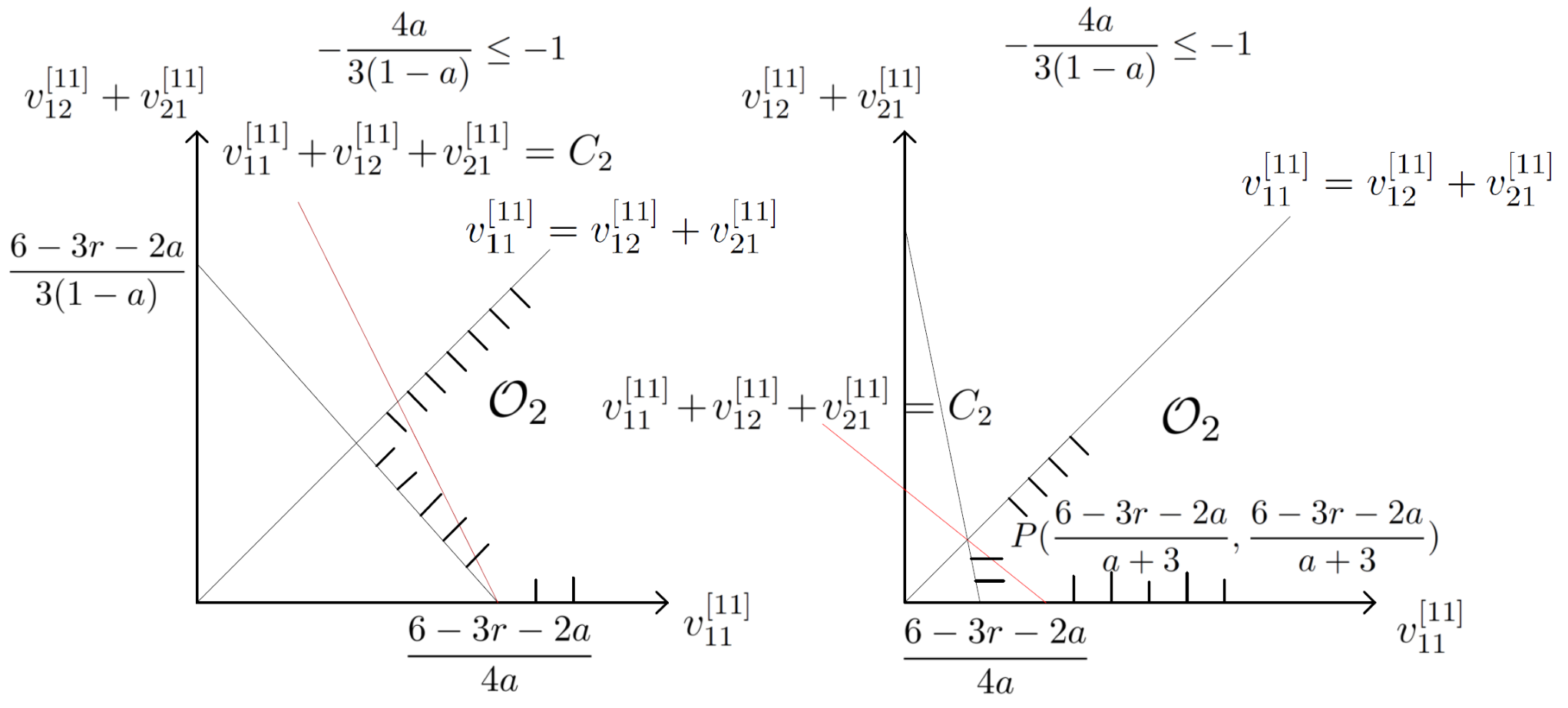
Fig. 11: The description of 𝒪2+\mathcal{O}_{2}^{+} and inf(v11[11],…,v22[11])∈𝒪2+v11[11]+v12[11]+v21[11]\inf_{(v_{11}^{[11]},\ldots,v_{22}^{[11]})\in\mathcal{O}_{2}^{+}}v_{11}^{[11]}+v_{12}^{[11]}+v_{21}^{[11]} depending on −4​a3​(1−a)-\frac{4a}{3(1-a)}.

If v11[11]+v22[11]≥v12[11]+v21[11]v_{11}^{[11]}+v_{22}^{[11]}\geq v_{12}^{[11]}+v_{21}^{[11]}, Pr{ℰI​A1}≐Pr{4a(1−v11[11])+3(−a)(−v12[11]−v21[11])<3r}≐Pr{4av11[11]+3(1−a)(v12[11]+v21[11])>−3r−2a}.\textrm{Pr}\{\mathcal{E}_{IA_{1}}\}\!\doteq\!\textrm{Pr}\Big\{\!4a(1-v_{11}^{[11]})+\!3(\!1\!-\!a\!)(2\!-\!v_{12}^{[11]}\!-\!v_{21}^{[11]})<3r\Big\}\doteq\textrm{Pr}\Big\{\!4av_{11}^{[11]}+3(1-a)(v_{12}^{[11]}+v_{21}^{[11]})\!\!>\!6\!-\!3r\!-\!2a\!\Big\}. Let us define an outage set, 𝒪2={(v11[11],…,v22[11])|4​a​v11[11]+3​(1−a)​(v12[11]+v21[11])>6−3​r−2​a}\mathcal{O}_{2}=\{(v_{11}^{[11]},\ldots,v_{22}^{[11]})|4av_{11}^{[11]}+3(1-a)(v_{12}^{[11]}+v_{21}^{[11]})>6-3r-2a\}. In a similar way to the case when v11[11]+v22[11]<v12[11]+v21[11]v_{11}^{[11]}+v_{22}^{[11]}<v_{12}^{[11]}+v_{21}^{[11]},

Pr​{ℰI​A1}\displaystyle\textrm{Pr}\{\mathcal{E}_{IA_{1}}\} ≐ρ−inf(v11[11],…,v22[11])∈𝒪2+∑m,n=,1,2vm​n[11]\displaystyle\doteq\rho^{-\inf_{(v_{11}^{[11]},\ldots,v_{22}^{[11]})\in\mathcal{O}_{2}^{+}}\sum_{m,n=,1,2}v_{mn}^{[11]}}
≐(b)ρ−inf(v11[11],…,v22[11])∈𝒪2+(v11[11]+v12[11]+v21[11]),\displaystyle\stackrel{{\scriptstyle(\textrm{b})}}{{\doteq}}\rho^{-\inf_{(v_{11}^{[11]},\ldots,v_{22}^{[11]})\in\mathcal{O}_{2}^{+}}(v_{11}^{[11]}+v_{12}^{[11]}+v_{21}^{[11]})}, (75)

where (b) follows from v22[11]>0v_{22}^{[11]}>0. When (b) holds, the condition v11[11]+v22[11]≥v12[11]+v21[11]v_{11}^{[11]}+v_{22}^{[11]}\geq v_{12}^{[11]}+v_{21}^{[11]} is reduced to v11[11]≥v12[11]+v21[11]v_{11}^{[11]}\geq v_{12}^{[11]}+v_{21}^{[11]} since outage set 𝒪2\mathcal{O}_{2} is not dependent on v22[11]v_{22}^{[11]} and infv22[11]>0v22[11]=0\inf_{v_{22}^{[11]}>0}v_{22}^{[11]}=0. Let v11[11]+v12[11]+v21[11]=C2v_{11}^{[11]}+v_{12}^{[11]}+v_{21}^{[11]}=C_{2}. Then, using a plane with v11[11]v_{11}^{[11]} and v12[11]+v21[11]v_{12}^{[11]}+v_{21}^{[11]} axes in Fig. 11, we can obtain the dominant scale of Pr​{ℰI​A1}\textrm{Pr}\{\mathcal{E}_{IA_{1}}\}, when v11[11]+v22[11]≥v12[11]+v21[11]v_{11}^{[11]}+v_{22}^{[11]}\geq v_{12}^{[11]}+v_{21}^{[11]}, as Pr​{ℰI​A1}≐ρ−min⁡(2a+3,14​a)​(6−3​r−2​a).\textrm{Pr}\{\mathcal{E}_{IA_{1}}\}\doteq\rho^{-\min(\frac{2}{a+3},\frac{1}{4a})(6-3r-2a)}.

Therefore, combining the two cases when v11[11]+v22[11]<v12[11]+v21[11]v_{11}^{[11]}+v_{22}^{[11]}<v_{12}^{[11]}+v_{21}^{[11]} and when v11[11]+v22[11]≥v12[11]+v21[11]v_{11}^{[11]}+v_{22}^{[11]}\geq v_{12}^{[11]}+v_{21}^{[11]}, we obtain the dominant scale of Pr​{ℰI​A1}\textrm{Pr}\{\mathcal{E}_{IA_{1}}\} as

Pr​{ℰI​A1}\displaystyle\textrm{Pr}\{\mathcal{E}_{IA_{1}}\} ≐ρ−min⁡(23​(1−a),2a+3,14​a)​(6−3​r−2​a)\displaystyle\doteq\rho^{-\min(\frac{2}{3(1-a)},\frac{2}{a+3},\frac{1}{4a})(6-3r-2a)}
≐ρ−min⁡(2a+3,14​a)​(6−3​r−2​a),\displaystyle\doteq\rho^{-\min(\frac{2}{a+3},\frac{1}{4a})(6-3r-2a)}, (76)

since 2a+3≤23​(1−a)\frac{2}{a+3}\leq\frac{2}{3(1-a)} for 0≤a≤10\leq a\leq 1.

Now, we calculate the dominant scale of Pr​{ℰI​A2}\textrm{Pr}\{\mathcal{E}_{IA_{2}}\}. If v1​k1[1​l1]=v11[11]v_{1k_{1}}^{[1l_{1}]}=v_{11}^{[11]}, the number of independent random variables involved in (III-B) is 3; otherwise, i.e., v1​k1[1​l1]≠v11[11]v_{1k_{1}}^{[1l_{1}]}\neq v_{11}^{[11]}, the number of independent random variables involved in (III-B) is 4.

Refer to caption
Fig. 12: The description of 𝒪3+\mathcal{O}_{3}^{+} and inf(v11[11],…,v22[11])∈𝒪3+4​(v11[11]+v22[11])+v11[22]\inf_{(v_{11}^{[11]},\ldots,v_{22}^{[11]})\in\mathcal{O}_{3}^{+}}4(v_{11}^{[11]}+v_{22}^{[11]})+v_{11}^{[22]} depending on (a+3)​v11[11]+3​(1−a)​v22[11]+4​a​v11[22]=6−6​r+2​a(a+3)v_{11}^{[11]}+3(1-a)v_{22}^{[11]}+4av_{11}^{[22]}=6-6r+2a.

Firstly, we consider the case when v1​k1[1​l1]=v11[11]v_{1k_{1}}^{[1l_{1}]}=v_{11}^{[11]}. In this case. v2​k2[1​l2]v_{2k_{2}}^{[1l_{2}]} can be v21[12]v_{21}^{[12]}, v22[11]v_{22}^{[11]}, or v22[12]v_{22}^{[12]}. Since v21[12]v_{21}^{[12]}, v22[11]v_{22}^{[11]}, and v22[12]v_{22}^{[12]} are i.i.d., and dominant scale of Pr​{ℰI​A2}\textrm{Pr}\{\mathcal{E}_{IA_{2}}\} is the same whatever v2​k2[1​l2]v_{2k_{2}}^{[1l_{2}]} is among the three possible candidates, without loss of generality, we consider only one of the candidates, v2​k2[1​l2]=v22[11]v_{2k_{2}}^{[1l_{2}]}=v_{22}^{[11]}. Then, since

minl1,l2,k1,k2∈{1,2}​⋂(l1,k1)≠(l2,k2)⁡v1​k1[1​l1]+v2​k2[1​l2]=v11[11]+v22[11],\displaystyle\min_{l_{1},l_{2},k_{1},k_{2}\in\{1,2\}\bigcap(l_{1},k_{1})\neq(l_{2},k_{2})}v_{1k_{1}}^{[1l_{1}]}+v_{2k_{2}}^{[1l_{2}]}=v_{11}^{[11]}+v_{22}^{[11]}, (77)

the dominant scale of the outage probability of ℰI​A2\mathcal{E}_{IA_{2}} becomes

Pr​{ℰI​A2}\displaystyle\textrm{Pr}\{\mathcal{E}_{IA_{2}}\} ≐Pr{ρ4​a3​(1−a)​(2−v11[11]−v11[22])+2−v11[11]−v22[11]<ρ2​r1−a}\displaystyle\doteq\textrm{Pr}\Big\{\rho^{\frac{4a}{3(1-a)}(2-v_{11}^{[11]}-v_{11}^{[22]})+2-v_{11}^{[11]}-v_{22}^{[11]}}<\rho^{\frac{2r}{1-a}}\Big\}
≐Pr{(a+3)v11[11]+3(1−a)v22[11]+4av11[22]\displaystyle\doteq\textrm{Pr}\Big\{(a+3)v_{11}^{[11]}+3(1-a)v_{22}^{[11]}+4av_{11}^{[22]}
>6−6r+2a}.\displaystyle~~~~~~>6-6r+2a\Big\}. (78)

Let us define an outage set, 𝒪3={(v11[11],…,v22[12],v11[22])|(a+3)​v11[11]+3​(1−a)​v22[11]+4​a​v11[22]>6−6​r+2​a}\mathcal{O}_{3}=\{(v_{11}^{[11]},\ldots,v_{22}^{[12]},v_{11}^{[22]})|(a+3)v_{11}^{[11]}+3(1-a)v_{22}^{[11]}+4av_{11}^{[22]}>6-6r+2a\}, in terms of the associated exponential variables. Then, from (5),

Pr​{ℰI​A2}\displaystyle\textrm{Pr}\{\mathcal{E}_{IA_{2}}\} ≐ρ−inf(v11[11],…,v22[12],v11[22])∈𝒪3+∑p,q,r=1,2v1​p[q​r]+v11[22]\displaystyle\doteq\rho^{-\inf_{(v_{11}^{[11]},\ldots,v_{22}^{[12]},v_{11}^{[22]})\in\mathcal{O}_{3}^{+}}\sum_{p,q,r=1,2}v_{1p}^{[qr]}+v_{11}^{[22]}}
≐(c)ρ−inf(v11[11],…,v22[12],v11[22])∈𝒪3+4(v11[11]+v22[11])+v11[22],\displaystyle\stackrel{{\scriptstyle(\textrm{c})}}{{\doteq}}\rho^{-\inf_{(v_{11}^{[11]},\ldots,v_{22}^{[12]},v_{11}^{[22]})\in\mathcal{O}_{3}^{+}}4(v_{11}^{[11]}+v_{22}^{[11]})+v_{11}^{[22]}},

where (c) follows from (77). Let 4​(v11[11]+v22[11])+v11[22]=C34(v_{11}^{[11]}+v_{22}^{[11]})+v_{11}^{[22]}=C_{3}. Then, as illustrated in Fig. 12, since both 4​(v11[11]+v22[11])+v11[22]=C34(v_{11}^{[11]}+v_{22}^{[11]})+v_{11}^{[22]}=C_{3} and (a+3)​v11[11]+3​(1−a)​v22[11]+4​a​v11[22]=6−6​r+2​a(a+3)v_{11}^{[11]}+3(1-a)v_{22}^{[11]}+4av_{11}^{[22]}=6-6r+2a are planes in the three-dimensional space, infC3\inf C_{3} is found at a point on v11[11]v_{11}^{[11]}, v11[22]v_{11}^{[22]}, or v22[11]v_{22}^{[11]} axis, which correspond to cases (A), (B), and (C) in Fig. 12; For case (A), infC3\inf C_{3} is found at (0,6−6​r+2​aa+3,0)(0,\frac{6-6r+2a}{a+3},0) on v11[11]v_{11}^{[11]} axis. Hence, the dominant scale of Pr​{ℰI​A2}\textrm{Pr}\{\mathcal{E}_{IA_{2}}\} is represented as ρ−inf(v11[11],…,v22[12],v11[22])∈𝒪3+4v11[11]≐ρ−4​(6−6​r+2​a)a+3.\rho^{-\inf_{(v_{11}^{[11]},\ldots,v_{22}^{[12]},v_{11}^{[22]})\in\mathcal{O}_{3}^{+}}4v_{11}^{[11]}}\doteq\rho^{-\frac{4(6-6r+2a)}{a+3}}. For case (B), infC3\inf C_{3} is found at (6−6​r+2​a4​a,0,0)(\frac{6-6r+2a}{4a},0,0) on v11[22]v_{11}^{[22]} axis, and the dominant scale of Pr​{ℰI​A2}\textrm{Pr}\{\mathcal{E}_{IA_{2}}\} is represented as ρ−inf(v11[11],…,v22[12],v11[22])∈𝒪3+v11[22]≐ρ−(6−6​r+2​a)4​a.\rho^{-\inf_{(v_{11}^{[11]},\ldots,v_{22}^{[12]},v_{11}^{[22]})\in\mathcal{O}_{3}^{+}}v_{11}^{[22]}}\doteq\rho^{-\frac{(6-6r+2a)}{4a}}. For case (C), infC3\inf C_{3} is found at (0,0,6−6​r+2​a3​(1−a))(0,0,\frac{6-6r+2a}{3(1-a)}) on v22[11]v_{22}^{[11]} axis, and similarly, the dominant scale of Pr​{ℰI​A2}\textrm{Pr}\{\mathcal{E}_{IA_{2}}\} is represented as ρ−inf(v11[11],…,v22[12],v11[22])∈𝒪3+4v22[11]≐ρ−4​(6−6​r+2​a)3​(1−a).\rho^{-\inf_{(v_{11}^{[11]},\ldots,v_{22}^{[12]},v_{11}^{[22]})\in\mathcal{O}_{3}^{+}}4v_{22}^{[11]}}\doteq\rho^{-\frac{4(6-6r+2a)}{3(1-a)}}.

Pr​{ℰI​A2}\displaystyle\textrm{Pr}\{\mathcal{E}_{IA_{2}}\} ≐ρ−min⁡(43​(1−a),4a+3,14​a)​(6−6​r+2​a)\displaystyle\doteq\rho^{-\min(\frac{4}{3(1-a)},\frac{4}{a+3},\frac{1}{4a})(6-6r+2a)}
≐ρ−min⁡(4a+3,14​a)​(6−6​r+2​a),\displaystyle\doteq\rho^{-\min(\frac{4}{a+3},\frac{1}{4a})(6-6r+2a)}, (79)

since 43​(1−a)​(6−6​r+2​a)≥4a+3​(6−6​r+2​a),∀r,0≤a≤1\frac{4}{3(1-a)}(6-6r+2a)\geq\frac{4}{a+3}(6-6r+2a),\forall r,0\leq a\leq 1.

Secondly, we consider the case when v1​k1[1​l1]≠v11[11]v_{1k_{1}}^{[1l_{1}]}\neq v_{11}^{[11]}. If v1​k1[1​l1]≠v11[11]v_{1k_{1}}^{[1l_{1}]}\neq v_{11}^{[11]}, the number of possible pairs of (v1​k1[1​l1],v2​k2[1​l2])(v_{1k_{1}}^{[1l_{1}]},v_{2k_{2}}^{[1l_{2}]}) resulting in the same value of minl1,l2,k1,k2∈{1,2}​⋂(l1,k1)≠(l2,k2)⁡v1​k1[1​l1]+v2​k2[1​l2]\min_{l_{1},l_{2},k_{1},k_{2}\in\{1,2\}\bigcap(l_{1},k_{1})\neq(l_{2},k_{2})}v_{1k_{1}}^{[1l_{1}]}+v_{2k_{2}}^{[1l_{2}]} is 9. Therefore, similar to the case when v1​k1[1​l1]=v11[11]v_{1k_{1}}^{[1l_{1}]}=v_{11}^{[11]}, we consider only one of the possible 9 candidates that

minl1,l2,k1,k2∈{1,2}​⋂(l1,k1)≠(l2,k2)⁡v1​k1[1​l1]+v2​k2[1​l2]=v11[12]+v22[11].\displaystyle\min_{l_{1},l_{2},k_{1},k_{2}\in\{1,2\}\bigcap(l_{1},k_{1})\neq(l_{2},k_{2})}v_{1k_{1}}^{[1l_{1}]}+v_{2k_{2}}^{[1l_{2}]}=v_{11}^{[12]}+v_{22}^{[11]}. (80)

With (80), the dominant scale of the outage probability of ℰI​A2\mathcal{E}_{IA_{2}} becomes

Pr​{ℰI​A2}\displaystyle\textrm{Pr}\{\mathcal{E}_{IA_{2}}\} ≐Pr{ρ4​a3​(1−a)​(2−v11[11]−v11[22])+2−v11[12]−v22[11]<ρ2​r1−a}\displaystyle\doteq\textrm{Pr}\Big\{\rho^{\frac{4a}{3(1-a)}(2-v_{11}^{[11]}-v_{11}^{[22]})+2-v_{11}^{[12]}-v_{22}^{[11]}}<\rho^{\frac{2r}{1-a}}\Big\}
≐Pr{3(1−a)(v11[12]+v22[11])+4a(v11[11]+v11[22])\displaystyle\doteq\textrm{Pr}\Big\{3(1-a)(v_{11}^{[12]}+v_{22}^{[11]})+4a(v_{11}^{[11]}+v_{11}^{[22]})
>6−6r+2a}.\displaystyle~~~~~>6-6r+2a\Big\}. (81)

Let us define an outage set, 𝒪4={(v11[11],…,v22[12],v11[22])|3​(1−a)​(v11[12]+v22[11])+4​a​(v11[11]+v11[22])>6−6​r+2​a}\mathcal{O}_{4}=\{(v_{11}^{[11]},\ldots,v_{22}^{[12]},v_{11}^{[22]})|3(1-a)(v_{11}^{[12]}+v_{22}^{[11]})+4a(v_{11}^{[11]}+v_{11}^{[22]})>6-6r+2a\}, in terms of the associated exponential variables. Then, from (5),

Pr​{ℰI​A2}\displaystyle\textrm{Pr}\{\mathcal{E}_{IA_{2}}\}\! ≐ρ−inf(v11[11],…,v22[12],v11[22])∈𝒪4+∑p,q,r=1,2v1​p[q​r]+v11[22]\displaystyle\doteq\rho^{-\inf_{(v_{11}^{[11]},\ldots,v_{22}^{[12]},v_{11}^{[22]})\in\mathcal{O}_{4}^{+}}\sum_{p,q,r=1,2}v_{1p}^{[qr]}+v_{11}^{[22]}} (82)
≐(d)ρ−inf(v11[11],…,v22[12],v11[22])∈𝒪4+3(v11[12]+v22[11])+v11[11]+v12[12]+v11[22]\displaystyle\stackrel{{\scriptstyle(\textrm{d})}}{{\doteq}}\!\rho^{\!\!\!-\inf_{(v_{11}^{[11]},\!\ldots,v_{22}^{[12]}\!,v_{11}^{[22]})\in\mathcal{O}_{4}^{+}}\!\!3(v_{11}^{[12]}\!+v_{22}^{[11]})\!+v_{11}^{[11]}\!\!+v_{12}^{[12]}\!\!+v_{11}^{[22]}} (83)
≐(e)ρ−inf(v11[11],…,v22[12],v11[22])∈𝒪4+3(v11[12]+v22[11])+v11[11]+v11[22],\displaystyle\stackrel{{\scriptstyle(\textrm{e})}}{{\doteq}}\rho^{\!\!-\inf_{(v_{11}^{[11]},\ldots,v_{22}^{[12]},v_{11}^{[22]})\in\mathcal{O}_{4}^{+}}3(v_{11}^{[12]}+v_{22}^{[11]})+v_{11}^{[11]}+v_{11}^{[22]}}, (84)

where (d) follows from (80) that v11[12]+v22[11]≤v12[11]+v21[12]v_{11}^{[12]}+v_{22}^{[11]}\leq v_{12}^{[11]}+v_{21}^{[12]}, v21[11]+v22[12]v_{21}^{[11]}+v_{22}^{[12]}, and (e) follows from infv12[12]>0v12[12]=0\inf_{v_{12}^{[12]}>0}v_{12}^{[12]}=0. Since infv12[12]>0v12[12]=0\inf_{v_{12}^{[12]}>0}v_{12}^{[12]}=0, the condition that v11[12]+v22[11]≤v11[11]+v12[12]v_{11}^{[12]}+v_{22}^{[11]}\leq v_{11}^{[11]}+v_{12}^{[12]} from (80) reduces to v11[12]+v22[11]≤v11[11]v_{11}^{[12]}+v_{22}^{[11]}\leq v_{11}^{[11]} in finding the dominant scale of Pr​{ℰI​A2}\textrm{Pr}\{\mathcal{E}_{IA_{2}}\}.

Refer to caption
Fig. 13: The description of 𝒪4+\mathcal{O}_{4}^{+} and inf(v11[11],…,v22[12],v11[22])∈𝒪4+3​(v11[12]+v22[11])+v11[11]+v11[22]\inf_{(v_{11}^{[11]},\ldots,v_{22}^{[12]},v_{11}^{[22]})\in\mathcal{O}_{4}^{+}}3(v_{11}^{[12]}+v_{22}^{[11]})+v_{11}^{[11]}+v_{11}^{[22]} depending on 3​(1−a)​(v11[12]+v22[11])+4​a​(v11[11]+v11[22])=6−6​r+2​a3(1-a)(v_{11}^{[12]}+v_{22}^{[11]})+4a(v_{11}^{[11]}+v_{11}^{[22]})=6-6r+2a under v11[12]+v22[11]<v11[11]v_{11}^{[12]}+v_{22}^{[11]}<v_{11}^{[11]}.

Let 3​(v11[12]+v22[11])+v11[11]+v11[22]=C43(v_{11}^{[12]}+v_{22}^{[11]})+v_{11}^{[11]}+v_{11}^{[22]}=C_{4}. Then, as illustrated in Fig. 13, both 3​(v11[12]+v22[11])+v11[11]+v11[22]=C43(v_{11}^{[12]}+v_{22}^{[11]})+v_{11}^{[11]}+v_{11}^{[22]}=C_{4} and 3​(1−a)​(v11[12]+v22[11])+4​a​(v11[11]+v11[22])=6−6​r+2​a3(1-a)(v_{11}^{[12]}+v_{22}^{[11]})+4a(v_{11}^{[11]}+v_{11}^{[22]})=6-6r+2a are planes in the three-dimensional space. Under v11[12]+v22[11]≤v11[11]v_{11}^{[12]}+v_{22}^{[11]}\leq v_{11}^{[11]}, infC4\inf C_{4} can be found at (0,6−6​r+2​a4​a,0)(0,\frac{6-6r+2a}{4a},0), (6−6​r+2​aa+3,6−6​r+2​aa+3,0)(\frac{6-6r+2a}{a+3},\frac{6-6r+2a}{a+3},0), or (0,0,6−6​r+2​a4​a)(0,0,\frac{6-6r+2a}{4a}), which correspond to cases (A), (B), and (C) in Fig. 13, respectively; For case (A), infC4\inf C_{4} is found at (0,6−6​r+2​a4​a,0)(0,\frac{6-6r+2a}{4a},0) on v11[11]v_{11}^{[11]} axis and thus the dominant scale of Pr​{ℰI​A2}\textrm{Pr}\{\mathcal{E}_{IA_{2}}\} is represented as ρ−inf(v11[11],…,v22[12],v11[22])∈𝒪4+v11[11]≐ρ−6−6​r+2​a4​a.\rho^{-\inf_{(v_{11}^{[11]},\ldots,v_{22}^{[12]},v_{11}^{[22]})\in\mathcal{O}_{4}^{+}}v_{11}^{[11]}}\doteq\rho^{-\frac{6-6r+2a}{4a}}. For case (B), infC4\inf C_{4} is found at (6−6​r+2​aa+3,6−6​r+2​aa+3,0)(\frac{6-6r+2a}{a+3},\frac{6-6r+2a}{a+3},0) on v11[11]=v11[12]+v22[11]v_{11}^{[11]}=v_{11}^{[12]}+v_{22}^{[11]}, and the dominant scale of Pr​{ℰI​A2}\textrm{Pr}\{\mathcal{E}_{IA_{2}}\} is represented as ρ−inf(v11[11],…,v22[12],v11[22])∈𝒪4+3(v11[12]+v22[11])+v11[11]≐ρ−4​(6−6​r+2​a)a+3.\rho^{-\inf_{(v_{11}^{[11]},\ldots,v_{22}^{[12]},v_{11}^{[22]})\in\mathcal{O}_{4}^{+}}3(v_{11}^{[12]}+v_{22}^{[11]})+v_{11}^{[11]}}\doteq\rho^{-\frac{4(6-6r+2a)}{a+3}}. For case (C), infC4\inf C_{4} is found at (0,0,6−6​r+2​a4​a)(0,0,\frac{6-6r+2a}{4a}) on v11[22]v_{11}^{[22]} axis, and similarly, the dominant scale of Pr​{ℰI​A2}\textrm{Pr}\{\mathcal{E}_{IA_{2}}\} is represented as Pr{ℰI​A2}≐ρ−inf(v11[11],…,v22[12],v11[22])∈𝒪4+v11[22]≐ρ−(6−6​r+2​a)4​a.\textrm{Pr}\{\mathcal{E}_{IA_{2}}\}\doteq\rho^{-\inf_{(v_{11}^{[11]},\ldots,v_{22}^{[12]},v_{11}^{[22]})\in\mathcal{O}_{4}^{+}}v_{11}^{[22]}}\doteq\rho^{-\frac{(6-6r+2a)}{4a}}. Consequently, combining the three cases,

Pr​{ℰI​A2}\displaystyle\textrm{Pr}\{\mathcal{E}_{IA_{2}}\} ≐ρ−min⁡(4a+3,14​a)​(6−6​r+2​a).\displaystyle\doteq\rho^{-\min(\frac{4}{a+3},\frac{1}{4a})(6-6r+2a)}. (85)

Finally, the diversity gain of the on-off switched IA scheme with symbol extension is determined by the dominant scale of Pr​{ℰI​A1}\textrm{Pr}\{\mathcal{E}_{IA_{1}}\} and Pr​{ℰI​A2}\textrm{Pr}\{\mathcal{E}_{IA_{2}}\}, which is also bounded by the diversity gain of the point-to-point 2 ×\times 2 MIMO case given as d⁡(r)=inf𝜶∈𝒜∑i=12(2​i−1)​αid(r)=\inf_{\boldsymbol{\alpha}\in\mathcal{A}}\sum_{i=1}^{2}(2i-1)\alpha_{i} where 𝒜={𝜶∈ℝ2|α1≥α2≥0, and ∑i(1−αi)+<r}\mathcal{A}=\left\{\>\boldsymbol{\alpha}\in\mathbb{R}^{2}\>\Big|\quad\alpha_{1}\geq\alpha_{2}\geq 0,\text{ and }\sum_{i}(1-\alpha_{i})^{+}<r\>\right\} and αi\alpha_{i} is the exponential order of eigenvalue λi\lambda_{i} for i∈{1,2}i\in\{1,2\} [15]. Therefore, the diversity gain is determined as the minimum of d2,2∗​(r)d^{*}_{2,2}(r) and the dominant scale of Pr​{ℰI​A1}\textrm{Pr}\{\mathcal{E}_{IA_{1}}\} and Pr​{ℰI​A2}\textrm{Pr}\{\mathcal{E}_{IA_{2}}\}.

Appendix B Finding the Dominant Scale of Pr​{ℰI​A​A1}\textrm{Pr}\{\mathcal{E}_{IAA_{1}}\} and Pr​{ℰI​A​A2}\textrm{Pr}\{\mathcal{E}_{IAA_{2}}\}

Because all channels of two symmetric users are i.i.d., indices i,j,i,j, and kk do not affect the dominant scale of Pr​{ℰI​A​A}\textrm{Pr}\{\mathcal{E}_{IAA}\}. For that reason, considering only the case of i=j=k=1i=j=k=1 suffices for simple notation.

For ℰI​A​A1\mathcal{E}_{IAA_{1}}, the outage probability is represented as

Pr​{ℰI​A​A1}\displaystyle\textrm{Pr}\{\mathcal{E}_{IAA_{1}}\} ≐Pr{43alog(+ρ(|h11[11]|2+|h11[12]|2))\displaystyle\!\doteq\!\textrm{Pr}\Big\{\frac{4}{3}a\log\left(1\!+\!\rho\left(\left|h_{11}^{[11]}\right|^{2}\!\!\!+\!\left|h_{11}^{[12]}\right|^{2}\right)\right)\!\!
+(−a)logdet(𝐈+ρ𝐇[11]𝐇[11]†)<rlogρ}\displaystyle+\!\!(1\!-\!a)\log\det\left(\mathbf{I}\!+\rho\mathbf{H}^{[11]}\mathbf{H}^{[11]\dagger}\right)\!<\!r\log\rho\Big\}
≐Pr{log(ρ1−v11[11]+ρ1−v11[12])4​a3​(1−a)\displaystyle\doteq\textrm{Pr}\Big\{\log\left(\rho^{1-v_{11}^{[11]}}+\rho^{1-v_{11}^{[12]}}\right)^{\frac{4a}{3(1-a)}}
+log(ρ2−v11[11]−v22[11]+ρ2−v12[11]−v21[11])<logρr1−a}\displaystyle+\log(\rho^{2-v_{11}^{[11]}-v_{22}^{[11]}}\!\!+\!\rho^{2-v_{12}^{[11]}-v_{21}^{[11]}})\!<\!\log\rho^{\frac{r}{1-a}}\!\Big\}
≤(f)Pr{log(ρ4​a3​(1−a)​(1−v11[11])+ρ4​a3​(1−a)​(1−v11[12]))\displaystyle\stackrel{{\scriptstyle(\textrm{f})}}{{\leq}}\textrm{Pr}\Big\{\log\left(\rho^{\frac{4a}{3(1-a)}(1-v_{11}^{[11]})}\!\!+\!\rho^{\frac{4a}{3(1-a)}(1-v_{11}^{[12]})}\right)\!\!
+log(ρ2−v11[11]−v22[11]+ρ2−v12[11]−v21[11])<logρr1−a}\displaystyle~+\!\log(\rho^{2-v_{11}^{[11]}-v_{22}^{[11]}}\!\!\!+\!\rho^{2-v_{12}^{[11]}-v_{21}^{[11]}})\!\!<\!\log\rho^{\frac{r}{1-a}}\!\Big\}
≐Pr{∑i=1,2{ρ4​a3​(1−a)​(1−v11[1​i])+2−v11[11]−v22[11]\displaystyle\doteq\textrm{Pr}\Big\{\sum_{i=1,2}\{\rho^{\frac{4a}{3(1-a)}(1-v_{11}^{[1i]})+2-v_{11}^{[11]}-v_{22}^{[11]}}
+ρ4​a3​(1−a)​(1−v11[1​i])+2−v12[11]−v21[11]}<ρr1−a},\displaystyle~+\rho^{\frac{4a}{3(1-a)}(1-v_{11}^{[1i]})+2-v_{12}^{[11]}-v_{21}^{[11]}}\}<\rho^{\frac{r}{1-a}}\Big\}, (86)

where (f) follows from (ρ1−v11[11]+ρ1−v11[12])4​a3​(1−a)≥ρ4​a3​(1−a)​(1−v11[11])+ρ4​a3​(1−a)​(1−v11[12])\left(\rho^{1-v_{11}^{[11]}}+\rho^{1-v_{11}^{[12]}}\right)^{\frac{4a}{3(1-a)}}\geq\rho^{\frac{4a}{3(1-a)}(1-v_{11}^{[11]})}+\rho^{\frac{4a}{3(1-a)}(1-v_{11}^{[12]})}.

Similar to proof of Theorem 1, we consider the two cases when v11[11]<v11[12]v_{11}^{[11]}<v_{11}^{[12]} and v11[11]≥v11[12]v_{11}^{[11]}\geq v_{11}^{[12]}. Omitting the details of calculation for economy of space, we have Pr​{ℰI​A​A1}≐ρ−min⁡(2a+3,23​(1−a),12​a)​(6−3​r−2​a)\textrm{Pr}\{\mathcal{E}_{IAA_{1}}\}\doteq\rho^{-\min(\frac{2}{a+3},\frac{2}{3(1-a)},\frac{1}{2a})(6-3r-2a)} when v11[11]<v11[12]v_{11}^{[11]}<v_{11}^{[12]}, whereas Pr​{ℰI​A​A1}≐ρ−min⁡(23​(1−a),12​a)​(6−3​r−2​a)\textrm{Pr}\{\mathcal{E}_{IAA_{1}}\}\doteq\rho^{-\min(\frac{2}{3(1-a)},\frac{1}{2a})(6-3r-2a)} when v11[11]≥v11[12]v_{11}^{[11]}\geq v_{11}^{[12]}. Combining the two cases, since 2a+3<23​(1−a)\frac{2}{a+3}<\frac{2}{3(1-a)} for 0≤a≤10\leq a\leq 1,

Pr​{ℰI​A​A1}\displaystyle\textrm{Pr}\{\mathcal{E}_{IAA_{1}}\} ≐ρ−min⁡(2a+3,23​(1−a),12​a)​(6−3​r−2​a)\displaystyle\doteq\rho^{-\min\left(\frac{2}{a+3},\frac{2}{3(1-a)},\frac{1}{2a}\right)(6-3r-2a)}
≐ρ−min⁡(2a+3,12​a)​(6−3​r−2​a).\displaystyle\doteq\rho^{-\min\left(\frac{2}{a+3},\frac{1}{2a}\right)(6-3r-2a)}. (87)

For ℰI​A​A2\mathcal{E}_{IAA_{2}}, the outage probability is given by

Pr​{ℰI​A​A2}\displaystyle\textrm{Pr}\{\mathcal{E}_{IAA_{2}}\} =Pr{∑i=1,243alog(+ρ(|h11[i​1]|2+|h11[i​2]|2))\displaystyle=\textrm{Pr}\Big\{\!\sum_{i=1,2}\frac{4}{3}a\log\!\left(1\!+\!\rho\!\left(\left|h_{11}^{[i1]}\right|^{2}\!\!+\!\left|h_{11}^{[i2]}\right|^{2}\right)\right)\!
+(1−a)logdet(1+ρ𝐇¯𝐇¯†)<2rlogρ}\displaystyle~+\!(1-a)\log\det\!\left(1+\rho\bar{\mathbf{H}}\bar{\mathbf{H}}^{\dagger}\right)\!<\!2r\log\rho\Big\}
≐Pr{log(∑i,j=1,2ρ2−v11[1​i]−v11[2​j])4​a3​(1−a)\displaystyle\doteq\textrm{Pr}\Big\{\log(\sum_{i,j=1,2}\rho^{2-v_{11}^{[1i]}-v_{11}^{[2j]}})^{\frac{4a}{3(1-a)}}
+log∑l1,l2,k1,k2∈{1,2}⋂(l1,k1)≠(l2,k2)ρ2−v1​k1[1​l1]−v2​k2[1​l2]<logρ2​r1−a}\displaystyle~+\log\!\!\!\!\!\sum\limits_{\scriptstyle l_{1},l_{2},k_{1},k_{2}\in\{1,2\}\atop\scriptstyle\bigcap(l_{1},k_{1})\neq(l_{2},k_{2})}\rho^{2-v_{1k_{1}}^{[1l_{1}]}-v_{2k_{2}}^{[1l_{2}]}}<\log\rho^{\frac{2r}{1-a}}\Big\}
≤Pr{log∑i,j=1,2ρ(2−v11[1​i]−v11[2​j])​4​a3​(1−a)\displaystyle\leq\textrm{Pr}\Big\{\log\sum_{i,j=1,2}\rho^{(2-v_{11}^{[1i]}-v_{11}^{[2j]})\frac{4a}{3(1-a)}}
+log∑l1,l2,k1,k2∈{1,2}⋂(l1,k1)≠(l2,k2)ρ2−v1​k1[1​l1]−v2​k2[1​l2]<logρ2​r1−a}.\displaystyle~+\log\!\!\!\!\!\sum\limits_{\scriptstyle l_{1},l_{2},k_{1},k_{2}\in\{1,2\}\atop\scriptstyle\bigcap(l_{1},k_{1})\neq(l_{2},k_{2})}\rho^{2-v_{1k_{1}}^{[1l_{1}]}-v_{2k_{2}}^{[1l_{2}]}}<\log\rho^{\frac{2r}{1-a}}\Big\}.

The dominant scale of Pr​{ℰI​A​A2}\textrm{Pr}\{\mathcal{E}_{IAA_{2}}\} is determine by the maximum scale among 48 possible combinations, similar to the on-off switched IA scheme based on the conventional IA. If we consider a specific case, by the similar way of the on-off switched IA scheme based on the conventional IA case, the dominant scale of Pr​{ℰI​A​A2}\textrm{Pr}\{\mathcal{E}_{IAA_{2}}\} is obtained as

Pr​{ℰI​A​A2}\displaystyle\textrm{Pr}\{\mathcal{E}_{IAA_{2}}\} ≐ρ−min⁡(43​(1−a),4a+3,12​a)​(6−6​r+2​a)\displaystyle\doteq\rho^{-\min(\frac{4}{3(1-a)},\frac{4}{a+3},\frac{1}{2a})(6-6r+2a)}
≐ρ−min⁡(4a+3,12​a)​(6−6​r+2​a).\displaystyle\doteq\rho^{-\min(\frac{4}{a+3},\frac{1}{2a})(6-6r+2a)}. (88)

We skip the detailed proof of finding the dominant scale of Pr​{ℰI​A​A2}\textrm{Pr}\{\mathcal{E}_{IAA_{2}}\} for economy of page space.

Finally, the diversity gain of the on-off switched IA with Alamouti coding scheme is determined by the dominant scale of Pr​{ℰI​A​A1}\textrm{Pr}\{\mathcal{E}_{IAA_{1}}\} and Pr​{ℰI​A​A2}\textrm{Pr}\{\mathcal{E}_{IAA_{2}}\}, which is also upper-bounded by the point-to-point 2 ×\times 2 MIMO DMT.

References

  • [1] Y.-b. Kim, M. G. Kang, and W. Choi, “Diversity-multiplexing tradeoff of the two-user X-channel with two antennas,” submitted to IEEE International Conference on Communications (ICC), Shanghai, China, May, 2019 .
  • [2] V. Cadambe and S. Jafar, “Interference alignment and the degrees of freedom for the KK user interference channel,” IEEE Trans. Inf. Theory, vol. 54, no. 8, pp. 3425-3441, Aug. 2008.
  • [3] S. Jafar and S. Shamai, “Degrees of freedom region for the MIMO X channel,” IEEE Trans. Inf. Theory, vol. 54, no. 1, pp. 151-170, Jan. 2008.
  • [4] V. Cadambe and S. Jafar, “Interference alignment and the degrees of freedom of wireless X networks,” IEEE Trans. Inf. Theory, vol. 55, no. 9, pp. 3893-3908, Sep. 2009.
  • [5] G. C. Alexandropoulos, P. Ferrand, J.-m. Gorce, and C. B. Papadias “Advanced coordinated beamforming for the downlink of future LTE cellular networks,” IEEE Communications Magazine, vol. 54, no. 7, pp. 54-60, Jul. 2016.
  • [6] F. Li and H. Jafarkhani, “Space-time processing for X channels using precoders,” IEEE Trans. Signal Process, vol. 60, no. 4, pp. 1849-1861, Apr. 2012.
  • [7] L. Shi, W. Zhang, and X. Xia, “Space-time block code design for two-user MIMO X channel,” IEEE Trans. Commun., vol. 61, no. 9, pp. 3806-3815, Sep. 2013.
  • [8] L. Li and H. Jafarkhani, “Maximum-rate transmission with improved diversity gain for interference networks,” IEEE Trans. Inf. Theory, vol. 59, no. 9, pp. 5313-5329, Sep. 2013.
  • [9] A. Ganesan and B. S. Rajan, “Interference alignment with diversity for the 2×2\times 2 X-network with three antennas,” in Proc. of IEEE ISIT, Jun./Jul. 2014, pp. 1216-1220.
  • [10] A. Ganesan and B. S. Rajan, “Interference alignment with diversity for the 2×\times2 X-network with four antennas,” IEEE Trans. Inf. Theory, vol. 60, no. 6, pp. 3576-3592, Jun. 2014.
  • [11] A. Ganesan and K. P. Srinath, “Interference aligned space-time transmission with diversity for the 2×\times2 X-network,” Available: http://arxiv.org/pdf/1501.04775v2.pdf, Jan. 2015.
  • [12] S. Alamouti, “A simple transmitter diversity scheme for wireless communications,” IEEE J. Sel. Areas Commun., vol. 16, no. 8, pp. 1451-1458, Oct. 1998.
  • [13] V. Tarokh, H. Jafarkhani, and A. Calderbank, “Space-time block codes from orthogonal designs,” IEEE Trans. Inf. Theory, vol. 45, no. 5, pp. 1456-1467, Jul. 1999.
  • [14] K. P. Srinath and B. S. Rajan, “Low ML-decoding complexity large coding gain, full-rate, full-diversity STBCs for 2×\times2 and 4×\times2 MIMO systems,” IEEE J. Sel. Topics Signal Process, vol. 3, no. 6, pp. 916-927, Dec. 2009.
  • [15] L. Zheng and D.N.C Tse, “Diversity and multiplexing: A fundamental tradeoff in multiple-antenna channels,” IEEE Trans. Inf. Theory, vol. 49, no. 5, pp. 1073-1096, May 2003.
  • [16] M. G. Kang, Y.-b. Kim, and W. Choi, “On the diversity multiplexing tradeoff in a 4-user clustered Z-channel,” in Proc. of Asilomar Conf. on Sig., Systems, and Computers, Montray, CA, Nov. 2012.
  • [17] Y.-b. Kim, M. G. Kang, and W. Choi, “On the achievable diversity multiplexing tradeoff of KK-user interference channels,” in Proc. of IEEE Globecom Workshop, Austin, Tx, Dec. 2014.
  • [18] A. Roostaei and M. Derakhtian, “Diversity-multiplexing tradeoff in an interweave multiuser cognitive radio system,” IEEE Trans. Wireless Commun., vol. 16, no. 1, pp. 389-399, Jan. 2017.
  • [19] F. Parvaresh and H. Soltanizadeh, “Diversity-multiplexing trade-off of half-duplex single relay networks,” IEEE Trans. Inf. Theory, vol. 63, no. 3, pp. 1703-1730, Mar. 2017.
  • [20] B. Bandemer, A. E. Gamal, and Y.-H. Kim, ”Simultaneous non-unique decoding is rate-optimal,” in Proc. of 2012 50th Annual Allerton Conference on Communication, Control, and Computing (Allerton), Monticello, IL, 2012, pp. 9-16.
  • [21] D. N. C Tse, P. Viswanath, and L. Zheng “Diversity-multiplexing tradeoff in multiple-access channels,” IEEE Trans. Inf. Theory, vol. 50, no. 9, pp. 1859-1874, Sep. 2004.
  • [22] A. Zaidi, Z. H. Awan, S. Shamai, and L. Vandendorpe, “Secure degrees of freedom of MIMO X-channels with output feedback and delayed CSIT,” IEEE Trans. on Inf. Forensics and Security, vol. 8, no. 11, pp. 1760-1774, Nov. 2013.
  • [23] A. Zaidi, Z. H. Awan, S. Shamai, and L. Vandendorpe, “Secure degrees of freedom of X-channel with output feedback and delayed CSI,” in Proc. of IEEE Int. Workshop on Information Theory (ITW), Sevilla, Spain, 2013.
[Uncaptioned image] Young-bin Kim (S’11-M’17) received the B.Sc. degree in Electrical Communications Engineering in 2008 and the M.Sc. and Ph.D. degree in Electrical Engineering from the Korea Advanced Institute of Science and Technology (KAIST), Daejeon, Korea, in 2010 and 2017, respectively. He was a Postdoctoral Research Scholar at KAIST from March to April in 2017. He is currently an Associate Research Engineer of KDDI Research, Inc., Saitama, Japan. He received the Korean Institute of Communications and Information Sciences (KICS) Outstanding Paper Award in 2016. He also received the IEICE 2018 Joint Conference on Satellite Communications Best Paper Award in 2018.
[Uncaptioned image] Myung Gil Kang (S’11-M’17) received the B.S. degree in Information and Communications Engineering, M.S. degree in electrical engineering and the Ph.D. degree in electrical engineering from the Korea Advanced Institute of Science and Technology (KAIST), Daejeon, Korea, in 2009, 2011, and 2017, respectively. He was a Post-Doctoral Research Scholar at KAIST from March 2017 to February 2018 and a Post-Doctoral Research Scholar at Hankuk University of Foreign Studies, Yongin, Korea from April 2018 to July 2018. He is currently a Post-Doctoral Research Scholar at Mid Sweden University, Sundsvall, Sweden. His research interests include signal processing, interference management, wireless security and information theory.
[Uncaptioned image] Wan Choi (S’03-M’06-SM’12) received the B.Sc. and M.Sc. degrees from the School of Electrical Engineering and Computer Science (EECS), Seoul National University (SNU), Seoul, Korea, in 1996 and 1998, respectively, and the Ph.D. degree in the Department of Electrical and Computer Engineering at the University of Texas at Austin in 2006. He is currently Professor of School of Electrical Engineering, Korea Advanced Institute of Science and Technology (KAIST), Daejeon, Korea. From 1998 to 2003, he was a Senior Member of the Technical Staff of the R&\&D Division of KT Freetel, Korea, where he researched 3G CDMA systems. He is the recipient of IEEE Vehicular Technology Society Jack Neubauer Memorial Award (Best System Paper Award) in 2002. He also received the IEEE Vehicular Technology Society Dan Noble Fellowship Award in 2006, the IEEE Communication Society Asia Pacific Young Researcher Award in 2007, and the Irwin-Jacobs Award from Qualcomm and KICS in 2015. While at the University of Texas at Austin, he was the recipient of William S. Livingston Graduate Fellowship and Information and Telecommunication Fellowship from Ministry of Information and Communication (MIC), Korea. He is an Executive Editor for the IEEE Transactions on Wireless Communications from Dec. 2014 and serves as Editor for the IEEE Transactions on Vehicular Technology. He also served as Editor for the IEEE Transactions on Wireless Communications (2009-2014), for the IEEE Wireless Communications Letter (2012-2017), and as Guest Editor for the 5G Wireless Communication System Special issue of the IEEE Journal on Selected Areas in Communications.