跳到论文正文
W Papers独立论文阅读器 arXiv:1811.08393 论文正文 计算阅读时间 · 0%
引用这篇论文根据当前论文元数据生成,正式投稿前建议核对。


License: arXiv.org perpetual non-exclusive license
arXiv:1811.08393v2 [cs.LG] 01 Feb 2020

Gen-Oja: A Two-time-scale approach for Streaming CCA

Kush Bhatia∗
University of California
Note: Equal contribution.
   Berkeley
kushbhatia@berkeley.edu
   Aldo Pacchiano∗
University of California
   Berkeley
pacchiano@berkeley.edu
   Nicolas Flammarion
University of California
   Berkeley
flammarion@berkeley.edu
   Peter L. Bartlett
University of California
   Berkeley
peter@berkeley.edu
   Michael I. Jordan
    University of California
   Berkeley
    jordan@cs.berkeley.edu
Abstract

In this paper, we study the problems of principal Generalized Eigenvector computation and Canonical Correlation Analysis in the stochastic setting. We propose a simple and efficient algorithm, Gen-Oja, for these problems. We prove the global convergence of our algorithm, borrowing ideas from the theory of fast-mixing Markov chains and two-time-scale stochastic approximation, showing that it achieves the optimal rate of convergence. In the process, we develop tools for understanding stochastic processes with Markovian noise which might be of independent interest.

1 Introduction

Cannonical Correlation Analysis (CCA) and the Generalized Eigenvalue Problem are two fundamental problems in machine learning and statistics, widely used for feature extraction in applications including regression [19], clustering [9] and classification [20].

Originally introduced by Hotelling in [17], CCA is a statistical tool for the analysis of multi-view data that can be viewed as a “correlation-aware" version of Principal Component Analysis (PCA). Given two multidimensional random variables, the objective in CCA is to obtain a pair of linear transformations that maximize the correlation between the transformed variables.

Given access to samples {(xi,yi)i=1n}\{(x_{i},y_{i})_{i=1}^{n}\} of zero mean random variables X,Y∈ℝdX,Y\in\mathbb{R}^{d} with an unknown joint distribution PX​YP_{XY}, CCA can be used to discover features expressing similarity or dissimilarity between XX and YY. Formally, CCA aims to find a pair of vectors u,v∈ℝdu,v\in\mathbb{R}^{d} such that projections of XX onto vv and YY onto uu are maximally correlated. In the population setting, the corresponding objective is given by:

max⁡v⊤​𝔼​[X​Y⊤]​us.t.v⊤​𝔼​[X​X⊤]​v=1​ and ​u⊤​𝔼​[Y​Y⊤]​u=1.\max v^{\top}\mathbb{E}[XY^{\top}]u\qquad\text{s.t.}\quad{{v^{\top}\mathbb{E}[XX^{\top}]v=1\text{ and }u^{\top}\mathbb{E}[YY^{\top}]u=1}}. (1)

In the context of covariance matrices, the objective of the generalized eigenvalue problem is to obtain the direction u​ or ​v∈ℝdu\text{ or }v\in\mathbb{R}^{d} maximizing discrepancy between XX and YY and can be formulated as,

arg⁡maxv≠0⁡v⊤​𝔼​[X​X⊤]​vv⊤​𝔼​[Y​Y⊤]​v​ and ​arg​maxu≠0​u⊤​𝔼​[Y​Y⊤]​uu⊤​𝔼​[X​X⊤]​u.\arg\max_{{v\neq 0}}\frac{v^{\top}\mathbb{E}[XX^{\top}]v}{v^{\top}\mathbb{E}[YY^{\top}]v}\text{ and }\arg\max_{{u\neq 0}}\frac{u^{\top}\mathbb{E}[YY^{\top}]u}{u^{\top}\mathbb{E}[XX^{\top}]u}. (2)

More generally, given symmetric matrices A,BA,B, with BB positive definite, the objective of the principal generalized eigenvector problem is to obtain a unit norm vector ww such that A​w=λ​B​wAw=\lambda Bw for λ\lambda maximal.

CCA and the generalized eigenvalue problem are intimately related. In fact, the CCA problem can be cast as a special case of the generalized eigenvalue problem by solving for uu and vv in the following objective:

(0𝔼⁡[X​Y⊤]𝔼⁡[Y​X⊤]0)⏟A​(vu)=λ​(𝔼⁡[X​X⊤]00𝔼⁡[Y​Y⊤])⏟B​(vu).\underbrace{\begin{pmatrix}0&\mathbb{E}[XY^{\top}]\\ \mathbb{E}[YX^{\top}]&0\end{pmatrix}}_{A}\begin{pmatrix}v\\ u\end{pmatrix}=\lambda\underbrace{\begin{pmatrix}\mathbb{E}[XX^{\top}]&0\\ 0&\mathbb{E}[YY^{\top}]\end{pmatrix}}_{B}\begin{pmatrix}v\\ u\end{pmatrix}. (3)

The optimization problems underlying both CCA and the generalized eigenvector problem are non-convex in general. While they admit closed-form solutions, even in the offline setting a direct computation requires 𝒪⁡(d3)\mathcal{O}(d^{3}) flops which is infeasible for large-scale datasets. Recently, there has been work on solving these problems by leveraging fast linear system solvers [15, 2] while requiring complete knowledge of the matrices AA and BB.

In the stochastic setting, the difficulty increases because the objective is to maximize a ratio of expectations, in contrast to the standard setting of stochastic optimization [27], where the objective is the maximization of an expectation. There has been recent interest in understanding and developing efficient algorithms with provable convergence guarantees for such non-convex problems. [18] and [28] recently analyzed the convergence rate of Oja’s algorithm [26], one of the most commonly used algorithm for streaming PCA.

In contrast, for the stochastic generalized eigenvalue problem and CCA problem, the focus has been to translate algorithms from the offline setting to the online one. For example, [12] proposes a streaming algorithm for the stochastic CCA problem which utilizes a streaming SVRG method to solve an online least-squares problem. Despite being streaming in nature, this algorithm requires a non-trivial initialization and, in contrast to the spirit of streaming algorithms, updates its eigenvector estimate only after every few samples. This raises the following challenging question:

  • Is it possible to obtain an efficient and provably convergent counterpart to Oja’s Algorithm for computing the principal generalized eigenvector in the stochastic setting?

In this paper, we propose a simple, globally convergent, two-line algorithm, Gen-Oja, for the stochastic principal generalized eigenvector problem and, as a consequence, we obtain a natural extension of Oja’s algorithm for the streaming CCA problem. Gen-Oja is an iterative algorithm which works by updating two coupled sequences at every time step. In contrast with existing methods [18], at each time step the algorithm can be seen as performing a step of Oja’s method, with a noise term which is neither zero mean nor conditionally independent, but instead is Markovian in nature. The analysis of the algorithm borrows tools from the theory of fast mixing of Markov chains [11] as well as two-time-scale stochastic approximation [6, 7, 8] to obtain an optimal (up to dimension dependence) fast convergence rate of 𝒪~​(1/n)\tilde{\mathcal{O}}(1/n). Our main contribution can summarized in the following informal theorem (made formal in Section 5).

Main Result (informal).

With probability greater than 4/54/5, one can obtain an ϵ\epsilon-accurate estimate of the generalized eigenvector in the stochastic setting using 𝒪~​(1/ϵ)\tilde{\mathcal{O}}(1/\epsilon) unbiased independent samples of the matrices. The multiplicative pre-factors depend polynomially on the inverse eigengap and the dimension of the problem.

Notation: We denote by λi​(M)\lambda_{i}(M) and σi​(M)\sigma_{i}(M) the it​hi^{th} largest eigenvalue and singular value of a square matrix MM. For any positive semi-definite matrix NN, we denote inner product in the NN-norm by ⟨⋅,⋅⟩N\langle\cdot,\cdot\rangle_{N} and the corresponding norm by ∥⋅∥N\|\cdot\|_{N}. We let κN=λmax​(N)λmin​(N)\kappa_{N}=\frac{\lambda_{\max}(N)}{\lambda_{\min}(N)} denote the condition number of NN. We denote the eigenvalues of the matrix B−1​AB^{-1}A by λ1>λ2≥…≥λd{\lambda_{1}>\lambda_{2}\geq\ldots\geq\lambda_{d}} with (ui)i=1d(u_{i})_{i=1}^{d} and (u~i)i=1d(\tilde{u}_{i})_{i=1}^{d} denoting the corresponding right and left eigenvectors of B−1​AB^{-1}A whose existence is guaranteed by Lemma 24 in Appendix G.3. We use Δλ\Delta_{\lambda} to denote the eigengap λ1−λ2\lambda_{1}-\lambda_{2}.

2 Problem Statement

In this section, we focus on the problem of estimating principal generalized eigenvectors in a stochastic setting. The generalized eigenvector, viv_{i}, corresponding to a system of matrices (A,B)(A,B), where A∈ℝd×dA\in\mathbb{R}^{d\times d} is a symmetric matrix and B∈ℝd×dB\in\mathbb{R}^{d\times d} is a symmetric positive definite matrix, satisfies

A​vi=λi​B​vi.Av_{i}=\lambda_{i}Bv_{i}. (4)

The principal generalized eigenvector v1v_{1} corresponds to the vector with the largest value11 1 Note that we consider here the largest signed value of λi\lambda_{i} of λi\lambda_{i}, or, equivalently, v1v_{1} is the principal eigenvector of the non-symmetric matrix B−1​AB^{-1}A. The vector v1v_{1} also corresponds to the maximizer of the generalized Rayleigh quotient given by

v1=arg⁡maxv∈ℝd⁡v⊤​A​vv⊤​B​v.v_{1}=\arg\max_{v\in\mathbb{R}^{d}}\frac{v^{\top}Av}{v^{\top}Bv}. (5)

In the stochastic setting, we only have access to a sequence of matrices A1,…,An∈ℝd×dA_{1},\dots,A_{n}\in\mathbb{R}^{d\times d} and B1,…,Bn∈ℝd×dB_{1},\dots,B_{n}\in\mathbb{R}^{d\times d} assumed to be drawn i.i.d. from an unknown underlying distribution, such that 𝔼⁡[Ai]=A\mathbb{E}[A_{i}]=A and 𝔼⁡[Bi]=B\mathbb{E}[B_{i}]=B and the objective is to estimate v1v_{1} given access to 𝒪⁡(d)\mathcal{O}(d) memory.

In order to quantify the error between a vector and its estimate, we define the following generalization of the sine with respect to the BB-norm as,

sinB2⁡(v,w)=1−(v⊤​B​w‖v‖B​‖w‖B)2.\sin^{2}_{B}(v,w)=1-\Big(\frac{v^{\top}Bw}{\|v\|_{B}\|w\|_{B}}\Big)^{2}. (6)

3 Related Work

PCA.

There is a vast literature dedicated to the development of computationally efficient algorithms for the PCA problem in the offline setting (see [24, 14] and references therein). In the stochastic setting, sharp convergence results were obtained recently by [18] and [28] for the principal eigenvector computation problem using Oja’s algorithm and later extended to the streaming k-PCA setting by [1]. They are able to obtain a 𝒪⁡(1/n)\mathcal{O}(1/n) convergence rate when the eigengap of the matrix is positive and a 𝒪⁡(1/n)\mathcal{O}(1/\sqrt{n}) rate is attained in the gap free setting.

Offline CCA and generalized eigenvector.

Computationally efficient optimization algorithms with finite convergence guarantees for CCA and the generalized eigenvector problem based on Empirical Risk Minimization (ERM) on a fixed dataset have recently been proposed in  [15, 32, 2]. These approaches work by reducing the CCA and generalized eigenvector problem to that of solving a PCA problem on a modified matrix MM (e.g., for CCA, M=B−12​A​B−12M=B^{\frac{-1}{2}}AB^{\frac{-1}{2}}). This reformulation is then solved by using an approximate version of the Power Method that relies on a linear system solver to obtain the approximate power method step. [15, 2] propose an algorithm for the generalized eigenvector computation problem and instantiate their results for the CCA problem. [21, 22, 32] focus on the CCA problem by optimizing a different objective:

min⁡12​𝔼^​|ϕ⊤​xi−ψ⊤​yi|2+λx​‖ϕ‖22+λy​‖ψ‖22 s.t. ‖ϕ‖𝔼^​[x​x⊤]=‖ψ‖𝔼^​[y​y⊤]=1,\min\frac{1}{2}\hat{\mathbb{E}}|\phi^{\top}x_{i}-\psi^{\top}y_{i}|^{2}+\lambda_{x}\|\phi\|_{2}^{2}+\lambda_{y}\|\psi\|_{2}^{2}\quad\text{ s.t. }\quad\|\phi\|_{\hat{\mathbb{E}}[xx^{\top}]}=\|\psi\|_{\hat{\mathbb{E}}[yy^{\top}]}=1,

where 𝔼^\hat{\mathbb{E}} denotes the empirical expectation. The proposed methods utilize the knowledge of complete data in order to solve the ERM problem, and hence is unclear how to extend them to the stochastic setting.

Stochastic CCA and generalized eigenvector.

There has been a dearth of work for solving these problems in the stochastic setting owing to the difficulties mentioned in Section 1. Recently, [12] extend the algorithm of [32] from the offline to the streaming setting by utilizing a streaming version of the SVRG algorithm for the least squares system solver. Their algorithm, based on the shift and invert method, suffers from two drawbacks: a) contrary to the spirit of streaming algorithms, this method does not update its estimate at each iteration – it requires to use logarithmic samples for solving an online least squares problem, and, b) their algorithm critically relies on obtaining an estimate of λ1\lambda_{1} to a small accuracy for which it requires to burn a few samples in the process. In comparison, Gen-Oja takes a single stochastic gradient step for the inner least squares problem and updates its estimate of the eigenvector after each sample. Perhaps the closest to our approach is [4], who propose an online method by solving a convex relaxation of the CCA objective with an inexact stochastic mirror descent algorithm. Unfortunately, the computational complexity of their method is 𝒪⁡(d2)\mathcal{O}(d^{2}) which renders it infeasible for large-scale problems.

4 Gen-Oja

Input: Time steps TT, step size αt\alpha_{t} (Least Squares), βt\beta_{t} (Oja)
Initialize: (w0,v0)←(w_{0},v_{0})\leftarrow sample uniformly from the unit sphere in ℝd\mathbb{R}^{d}, v¯0=v0\bar{v}_{0}=v_{0}
for t=1,…,Tt=1,\ldots,T do
Draw sample (At,Bt)(A_{t},B_{t})
    wt←wt−1−αt​(Bt​wt−1−At​vt−1)w_{t}\leftarrow w_{t-1}-\alpha_{t}(B_{t}w_{t-1}-A_{t}v_{t-1})
    vt′←vt−1+βt​wtv_{t}^{\prime}\leftarrow v_{t-1}+\beta_{t}w_{t}
    vt←vt′‖vt‖2v_{t}\leftarrow\frac{v_{t}^{\prime}}{\|v_{t}\|_{2}}
    Output: Estimate of Principal Generalized Eigenvector: vT{v}_{T}
Algorithm 1 Gen-Oja for Streaming A​v=λ​B​vAv=\lambda Bv

In this section, we describe our proposed approach for the stochastic generalized eigenvector problem (see Section 2). Our algorithm Gen-Oja, described in Algorithm 1, is a natural extension of the popular Oja’s algorithm used for solving the streaming PCA problem. The algorithm proceeds by iteratively updating two coupled sequences (wt,vt)(w_{t},v_{t}) at the same time: wtw_{t} is updated using one step of stochastic gradient descent with constant step-size to minimize w⊤​B​w−2​w⊤​A​vtw^{\top}Bw-2w^{\top}Av_{t} and vtv_{t} is updated using a step of Oja’s algorithm. Gen-Oja has its roots in the theory of two-time-scale stochastic approximation, by viewing the sequence wtw_{t} as a fast mixing Markov chain and vtv_{t} as a slowly evolving one. In the sequel, we describe the evolution of the Markov chains (wt)t≥0,(vt)t≥0(w_{t})_{t\geq 0},(v_{t})_{t\geq 0}, in the process outlining the intuition underlying Gen-Oja and understanding the key challenges which arise in the convergence analysis.

Oja’s algorithm.

Gen-Oja is closely related to the Oja’s algorithm [26] for the streaming PCA problem. Consider a special case of the problem, when each Bt=IB_{t}=I. In the offline setting, this reduces the generalized eigenvector problem to that of computing the principal eigenvector of A. With the setting of step-size αt=1\alpha_{t}=1, Gen-Oja recovers the Oja’s algorithm given by

vt=vt−1+βt​At​vt−1∥vt−1+βtAtvt−1.∥v_{t}=\frac{v_{t-1}+\beta_{t}A_{t}v_{t-1}}{\|v_{t-1}+\beta_{t}A_{t}v_{t-1}.\|}

This algorithm is exactly a projected stochastic gradient ascent on the Rayleigh quotient v⊤​A​vv^{\top}Av (with a step size βt\beta_{t}). Alternatively, it can be interpreted as a randomized power method on the matrix (I+βt​A)(I+\beta_{t}A)[16].

Two-time-scale approximation.

The theory of two-time-scale approximation forms the underlying basis for Gen-Oja. It considers coupled iterative systems where one component changes much faster than the other [7, 8]. More precisely, its objective is to understand classical systems of the type:

xt\displaystyle x_{t} =\displaystyle= xt−1+αt​[h⁡(xt−1,yt−1)+ξt1]\displaystyle x_{t-1}+\alpha_{t}\left[h\left(x_{t-1},y_{t-1}\right)+\xi^{1}_{t}\right] (7)
yt\displaystyle y_{t} =\displaystyle= yt−1+βt​[g⁡(xt−1,yt−1)+ξt2],\displaystyle y_{t-1}+\beta_{t}\left[g\left(x_{t-1},y_{t-1}\right)+\xi^{2}_{t}\right], (8)

where gg and hh are the update functions and (ξt1,ξt2)(\xi^{1}_{t},\xi^{2}_{t}) correspond to the noise vectors at step tt and typically assumed to be martingale difference sequences.

In the above model, whenever the two step sizes αt\alpha_{t} and βt\beta_{t} satisfy βt/αt→0\beta_{t}/\alpha_{t}\to 0, the sequence yty_{t} moves on a slower timescale than xtx_{t}. For any fixed value of yy the dynamical system given by xtx_{t},

xt=xt−1+αt​[h⁡(xt−1,y)+ξt1],x_{t}=x_{t-1}+\alpha_{t}[h\left(x_{t-1},y\right)+\xi^{1}_{t}], (9)

converges to to a solution x∗​(y)x^{*}(y). In the coupled system, since the state variables xtx_{t} move at a much faster time scale, they can be seen as being close to x∗​(yt)x^{*}(y_{t}), and thus, we can alternatively consider:

yt=yt−1+βt​[g⁡(x∗​(yt−1),yt−1)+ξt2].y_{t}=y_{t-1}+\beta_{t}\left[g\left(x_{*}(y_{t-1}),y_{t-1}\right)+\xi^{2}_{t}\right]. (10)

If the process given by yty_{t} above were to converge to y∗y^{*}, under certain conditions, we can argue that the coupled process (xt,yt)(x_{t},y_{t}) converges to (x∗​(y∗),y∗)(x^{*}(y^{*}),y^{*}). Intuitively, because xtx_{t} and yty_{t} are evolving at different time-scales, xtx_{t} views the process yty_{t} as quasi-constant while yty_{t} views xtx_{t} as a process rapidly converging to x∗​(yt)x^{*}(y_{t}).

Gen-Oja can be seen as a particular instance of the coupled iterative system given by Equations (7) and (8) where the sequence vtv_{t} evolves with a step-size βt≈1t\beta_{t}\approx\frac{1}{t}, much slower than the sequence wtw_{t}, which has a step-size of αt≈1log⁡(t)\alpha_{t}\approx\frac{1}{\log(t)}. Proceeding as above, the sequence vtv_{t} views wtw_{t} as having converged to B−1​A​vt+ξtB^{-1}Av_{t}+\xi_{t}, where ξt\xi_{t} is a noise term, and the update step for vtv_{t} in Gen-Oja can be viewed as a step of Oja’s algorithm, albeit with Markovian noise.

While previous works on the stochastic CCA problem required to use logarithmic independent samples to solve the inner least-squares problem in order to perform an approximate power method (or Oja) step, the theory of two-time-scale stochastic approximation suggests that it is possible to obtain a similar effect by evolving the sequences wtw_{t} and vtv_{t} at two different time scales.

Understanding the Markov Process {wt}\{w_{t}\}.

In order to understand the process described by the sequence wtw_{t}, we consider the homogeneous Markov chain (wtv)(w^{v}_{t}) defined by

wtv=wt−1v−α⁡(Bt​wt−1v−At​v),w^{v}_{t}=w^{v}_{t-1}-\alpha(B_{t}w^{v}_{t-1}-A_{t}v), (11)

for a constant vector vv and we denote its tt-step kernel by πvt\pi_{v}^{t} [23]. This Markov process is an iterative linear model and has been extensively studied by [29, 10, 5]. It is known that for any step-size α≤2/R2\alpha\leq 2/R^{2}, the Markov chain (wtv)t≥0(w^{v}_{t})_{t\geq 0} admits a unique stationary distribution, denoted by νv\nu_{v}. In addition,

W22​(πvt​(w0,⋅),νv)≤(1−2​μ​α​(1−α​RB2/2))t​∫ℝd‖w0−w‖22​d​νv​(w),W_{2}^{2}(\pi^{t}_{v}(w_{0},\cdot),\nu_{v})\leq(1-2\mu\alpha(1-\alpha R^{2}_{B}/2))^{t}\int_{\mathbb{R}^{d}}\|w_{0}-w\|_{2}^{2}d\nu_{v}(w), (12)

where W22​(λ,ν)W_{2}^{2}(\lambda,\nu) denotes the Wasserstein distance of order 2 between probability measures λ\lambda and ν\nu (see, e.g., [31] for more properties of W2W_{2}). Equation (12) implies that the iterative linear process described by (11) mixes exponentially fast to the stationary distribution. This forms a crucial ingredient in our convergence analysis where we use the fast mixing to obtain a bound on the expected norm of the Markovian noise (see Lemma 1).

Moreover, one can compute the mean w¯v\bar{w}^{v} of the process wtw_{t} under the stationary distribution by taking expectation under νv\nu_{v} on both sides in equation (11). Doing so, we obtain, w¯v=B−1​A​v\bar{w}^{v}=B^{-1}Av. Thus, in our setting, since the vtv_{t} process evolves slowly, we can expect that wt≈B−1​A​vtw_{t}\approx B^{-1}Av_{t}, allowing Gen-Oja to mimic Oja’s algorithm.

5 Main Theorem

In this section, we present our main convergence guarantee for Gen-Oja when applied to the streaming generalized eigenvector problem. We begin by listing the key assumptions required by our analysis:

(A1)

The matrices (Ai)i≥0(A_{i})_{i\geq 0} satisfy 𝔼⁡[Ai]=A\mathbb{E}[A_{i}]=A for a symmetric matrix A∈ℝd×dA\in\mathbb{R}^{d\times d}.

(A2)

The matrices (Bi)i≥0(B_{i})_{i\geq 0} are such that each Bi≽0B_{i}\succcurlyeq 0 is symmetric and satisfies 𝔼⁡[Bi]=B\mathbb{E}[B_{i}]=B for a symmetric matrix B∈ℝd×dB\in\mathbb{R}^{d\times d} with B≽μ​IB\succcurlyeq\mu I for μ>0\mu>0.

(A3)

There exists R≥0R\geq 0 such that max⁡{‖Ai‖,‖Bi‖}≤R\max\{\|A_{i}\|,\|B_{i}\|\}\leq R almost surely.

Under the assumptions stated above, we obtain the following convergence theorem for Gen-Oja with respect to the sin2B\sin^{2}_{B} distance, as described in Section 2.

Theorem 1 (Main Result).

Fix any δ>0\delta>0 and ϵ1>0\epsilon_{1}>0. Suppose that the step sizes are set to αt=clog⁡(d2​β+t)\alpha_{t}=\frac{c}{\log(d^{2}\beta+t)} and βt=γΔλ​(d2​β+t)\beta_{t}=\frac{\gamma}{\Delta_{\lambda}(d^{2}\beta+t)} for γ>1/2,c>1\gamma>1/2\ ,\ c>1 and

β=max⁡(20​γ2​λ12Δλ2​d2​log⁡(1+δ/1001+ϵ1),200​(Rμ+R3μ2+R5μ3)​log⁡(1+R2μ+R4μ2)δ​Δλ2).\beta=\max\left(\frac{20\gamma^{2}\lambda_{1}^{2}}{\Delta_{\lambda}^{2}d^{2}\log\left(\frac{1+\delta/100}{1+\epsilon_{1}}\right)},\frac{200\left(\frac{R}{\mu}+\frac{R^{3}}{\mu^{2}}+\frac{R^{5}}{\mu^{3}}\right)\log\left(1+\frac{R^{2}}{\mu}+\frac{R^{4}}{\mu^{2}}\right)}{\delta\Delta_{\lambda}^{2}}\right).

Suppose that the number of samples nn satisfy

d2​β+nlog1min⁡(1,2​γ​λ1/Δλ)⁡(d2​β+n)≥(c​dδ1​min⁡(1,λ1))1min⁡(1,2​γ​λ1/Δλ)​(d3​β+1)​exp⁡(c​λ12d2)\frac{d^{2}\beta+n}{\log^{\frac{1}{\min(1,2\gamma\lambda_{1}/\Delta_{\lambda})}}(d^{2}\beta+n)}\geq\left(\frac{cd}{\delta_{1}\min(1,\lambda_{1})}\right)^{\frac{1}{\min(1,2\gamma\lambda_{1}/\Delta_{\lambda})}}(d^{3}\beta+1)\exp\left(\frac{c\lambda_{1}^{2}}{d^{2}}\right)

Then, the output vnv_{n} of Algorithm 1 satisfies,

sinB2⁡(u1,vn)≤(2+ϵ1)​c​d​‖∑i=1du~i​u~i⊤‖2​log⁡(1δ)δ2​‖u~1‖22​(c​γ2​log3⁡(d2​β+n)Δλ2​(d2​β+n+1)+c​dΔλ​(d2​β+log3⁡(d2​β)d2​β+n+1)2​γ),\sin_{B}^{2}(u_{1},v_{n})\leq\frac{(2+\epsilon_{1})cd\|\sum_{i=1}^{d}\tilde{u}_{i}\tilde{u}_{i}^{\top}\|_{2}\log\left(\frac{1}{\delta}\right)}{\delta^{2}\|\tilde{u}_{1}\|_{2}^{2}}\left(\frac{c\gamma^{2}\log^{3}(d^{2}\beta+n)}{\Delta_{\lambda}^{2}(d^{2}\beta+n+1)}+\frac{cd}{\Delta_{\lambda}}\left(\frac{d^{2}\beta+\log^{3}(d^{2}\beta)}{d^{2}\beta+n+1}\right)^{2\gamma}\right),

with probability at least 1−δ1-\delta with cc depending polynomially on parameters of the problem λ1,κB,R,μ\lambda_{1},\kappa_{B},R,\mu. The parameter δ1\delta_{1} is set as δ1=ϵ12​(2+ϵ1)\delta_{1}=\frac{\epsilon_{1}}{2(2+\epsilon_{1})}.

The above result shows that with probability at least 1−δ1-\delta, Gen-Oja converges in the BB-norm to the right eigenvector, u1u_{1}, corresponding to the maximum eigenvalue of the matrix B−1​AB^{-1}A. Further, Gen-Oja exhibits an 𝒪~​(1/n)\tilde{\mathcal{O}}({1}/{n}) rate of convergence, which is known to be optimal for stochastic approximation algorithms even with convex objectives [25].

Comparison with Streaming PCA. In the setting where B=IB=I, and A⪰0A\succeq 0 is a covariance matrix, the principal generalized eigenvector problem reduces to performing PCA on the AA. When compared with the results obtained for streaming PCA by [18], our corresponding results differ by a factor of dimension dd and problem dependent parameters λ1,Δλ\lambda_{1},\Delta_{\lambda}. We believe that such a dependence is not inherent to Gen-Oja but a consequence of our analysis. We leave this task of obtaining a dimension free bound for Gen-Oja as future work.

Gap-independent step size: While the step size for the sequence vnv_{n} in Gen-Oja depends on eigen-gap, which is a priori unknown, one can leverage recent results as in [30] to get around this issue by using a streaming average step size.

6 Proof Sketch

In this section, we detail out the two key ideas underlying the analysis of Gen-Oja to obtain the convergence rate mentioned in Theorem 1: a) controlling the non i.i.d. Markovian noise term which is introduced because of the coupled Markov chains in Gen-Oja and b) proving that a noisy power method with such Markovian noise converges to the correct solution.

Controlling Markovian perturbations.

In order to better understand the sequence vtv_{t}, we rewrite the update as,

vt′=vt−1+βt​wt=vt−1+βt​(B−1​A​vt−1+ξt),v^{\prime}_{t}=v_{t-1}+\beta_{t}w_{t}=v_{t-1}+\beta_{t}(B^{-1}Av_{t-1}+\xi_{t}), (13)

where ξt=wt−B−1​A​vt−1\xi_{t}=w_{t}-B^{-1}Av_{t-1} is the prediction error which is a Markovian noise. Note that the noise term is neither mean zero nor a martingale difference sequence. Instead, the noise term ξt\xi_{t} is dependent on all previous iterates, which makes the analysis of the process more involved. This framework with Markovian noise has been extensively studied by [6, 3].

From the update in Equation (13), we observe that Gen-Oja is performing an Oja update but with a controlled Markovian noise. However, we would like to highlight that classical techniques in the study of stochastic approximation with Markovian noise (as the Poisson Equation [6, 23]) were not enough to provide adequate control on the noise to show convergence.

In order to overcome this difficulty, we leverage the fast mixing of the chain wtvw_{t}^{v} for understanding the Markovian noise. While it holds that 𝔼⁡[‖ξt‖2]=𝒪⁡(1)\mathbb{E}[\|\xi_{t}\|_{2}]=\mathcal{O}(1) (see Appendix C), a key part of our analysis is the following lemma, the proof of which can be found in Appendix B).

Lemma 1.

. For any choice of k>4​λ1​(B)μ​α​log⁡(1βt+k){k>4\frac{\lambda_{1}(B)}{\mu\alpha}\log(\frac{1}{\beta_{t+k}})}, and assuming that ‖ws‖≤Ws\|w_{s}\|\leq W_{s} for t≤s≤t+kt\leq s\leq t+k we have that

‖𝔼⁡[ξt+k|ℱt]‖2=𝒪⁡(βt​k2​αt​Wt+k)\|\mathbb{E}[\xi_{t+k}|\mathcal{F}_{t}]\|_{2}=\mathcal{O}(\beta_{t}k^{2}\alpha_{t}W_{t+k})

Lemma 1 uses the fast mixing of wtw_{t} to show that ∥𝔼[ξt]|ℱt−r∥2=𝒪~(βt)\|\mathbb{E}[\xi_{t}]|\mathcal{F}_{t-r}\|_{2}=\tilde{\mathcal{O}}(\beta_{t}) where r=𝒪⁡(log⁡t)r=\mathcal{O}(\log t), i.e., the magnitude of the expected noise is small conditioned on log⁡(t)\log(t) steps in the past.

Analysis of Oja’s algorithm.

The usual proofs of convergence for stochastic approximation define a Lyapunov function and show that it decreases sufficiently at each iteration. Oftentimes control on the per step rate of decrease can then be translated into a global convergence result. Unfortunately in the context of PCA, due to the non-convexity of the Raleigh quotient, the quality of the estimate vtv_{t} cannot be related to the previous vt−1v_{t-1}. Indeed vtv_{t} may become orthogonal to the leading eigenvector. Instead [18] circumvent this issue by leveraging the randomness of the initialization and adopt an operator view of the problem. We take inspiration from this approach in our analysis of Gen-Oja. Let Gi=wi​vi−1⊤G_{i}=w_{i}v_{i-1}^{\top} and Ht=∏i=1t(I+βi​Gi)H_{t}=\prod_{i=1}^{t}(I+\beta_{i}G_{i}), Gen-Oja’s update can be equivalently written as

vt=Ht​v0‖Ht​v0‖22,v_{t}=\frac{H_{t}v_{0}}{\|H_{t}v_{0}\|_{2}^{2}},

pushing, for the analysis only, the normalization step at the end. This point of view enables us to analyze the improvement of HtH_{t} over Ht−1H_{t-1} since allows one to interpret Oja’s update as one step of power method on HtH_{t} starting on a random vector v0v_{0}. We present here an easy adaptation of [18, Lemma 3.1] that takes into account the special geometry of the generalized eigenvector problem and the asymmetry of B−1​AB^{-1}A. The proof can be found in Appendix A.

Lemma 2.

Let H∈ℝd×dH\in\mathbb{R}^{d\times d}, (ui)i=1d(u_{i})_{i=1}^{d} and (u~i)i=1d(\tilde{u}_{i})_{i=1}^{d} be the corresponding right and left eigenvectors of B−1​AB^{-1}A and w∈ℝdw\in\mathbb{R}^{d} chosen uniformly on the sphere, then with probability 1−δ1-\delta (over the randomness in the initial iterate)

sinB2⁡(ui,H​w)≤C​log⁡(1/δ)δ​Tr⁡(H​H⊤​∑j≠iu~j​u~j⊤)u~i⊤​H​H⊤​u~i,\sin_{B}^{2}(u_{i},Hw)\leq\frac{C\log(1/\delta)}{\delta}\frac{\tr(HH^{\top}\sum_{j\neq i}\tilde{u}_{j}\tilde{u}_{j}^{\top})}{\tilde{u}_{i}^{\top}HH^{\top}\tilde{u}_{i}}, (14)

for some universal constant C>0C>0.

This lemma has the virtue of highly simplifying the challenging proof of convergence of Oja’s algorithm. Indeed we only have to prove that HtH_{t} will be close to ∏i=1t(I+βi​B−1​A)\prod_{i=1}^{t}(I+\beta_{i}B^{-1}A) for tt large enough which can be interpreted as an analogue of the law of large numbers for the multiplication of matrices. This will ensure that Tr⁡(Ht​Ht⊤​∑j≠iu~j​u~j⊤)\tr(H_{t}H_{t}^{\top}\sum_{j\neq i}\tilde{u}_{j}\tilde{u}_{j}^{\top}) is relatively small compared to u~i⊤​Ht​Ht⊤​u~i\tilde{u}_{i}^{\top}H_{t}H_{t}^{\top}\tilde{u}_{i} and be enough with Lemma 2 to prove Theorem 1. The proof follows the line of [18] with two additional tedious difficulties: the Markovian noise is neither unbiased nor independent of the previous iterates, and the matrix B−1​AB^{-1}A is no longer symmetric, which is precisely why we consider the left eigenvector u~i\tilde{u}_{i} in the right-hand side of Eq. (14). We highlight two key steps:

  • •

    First we show that 𝔼​Tr⁡(Ht​Ht⊤​∑j≠iu~j​u~j⊤)\mathbb{E}\tr(H_{t}H_{t}^{\top}\sum_{j\neq i}\tilde{u}_{j}\tilde{u}_{j}^{\top}) grows as 𝒪⁡(exp⁡(2​λ2​∑i=1tβi))\mathcal{O}(\exp(2\lambda_{2}\sum_{i=1}^{t}\beta_{i})), which implies by Markov’s inequality the same bound on Tr⁡(Ht​Ht⊤​∑j≠iu~j​u~j⊤)\tr(H_{t}H_{t}^{\top}\sum_{j\neq i}\tilde{u}_{j}\tilde{u}_{j}^{\top}) with constant probability. See Lemmas 16 for more details.

  • •

    Second we show that Var⁡u~i⊤​Ht​Ht⊤​u~i\Var\tilde{u}_{i}^{\top}H_{t}H_{t}^{\top}\tilde{u}_{i} grows as 𝒪⁡(exp⁡(4​λ1​∑i=1tβi))\mathcal{O}(\exp(4\lambda_{1}\sum_{i=1}^{t}\beta_{i})) and 𝔼​u~i⊤​H​H⊤​u~i\mathbb{E}\tilde{u}_{i}^{\top}HH^{\top}\tilde{u}_{i} grows as 𝒪⁡(exp⁡(2​λ1​∑i=1tβi))\mathcal{O}(\exp(2\lambda_{1}\sum_{i=1}^{t}\beta_{i})) which implies by Chebyshev’s inequality the same bound for u~i⊤​H​H⊤​u~i\tilde{u}_{i}^{\top}HH^{\top}\tilde{u}_{i} with constant probability. See Lemmas 17 and 19 for more details.

7 Application to Canonical Correlation Analysis

Consider two random vectors X∈ℝdX\in\mathbb{R}^{d} and Y∈ℝdY\in\mathbb{R}^{d} with joint distribution PX​YP_{XY}. The objective of canonical correlation analysis in the population setting is to find the canonical correlation vectors ϕ,ψ∈ℝd,d\phi,\psi\in\mathbb{R}^{d,d} which maximize the correlation

maxϕ,ψ⁡𝔼⁡[(ϕ⊤​X)​(ψ⊤​Y)]𝔼⁡[(ϕ⊤​X)2]​𝔼​[(ψ⊤​Y)2].\max_{\phi,\psi}\frac{\mathbb{E}[(\phi^{\top}X)(\psi^{\top}Y)]}{\sqrt{\mathbb{E}[(\phi^{\top}X)^{2}]\mathbb{E}[(\psi^{\top}Y)^{2}]}}.

This problem is equivalent to maximizing ϕ⊤​𝔼​[X​Y⊤]​ψ\phi^{\top}\mathbb{E}[XY^{\top}]\psi under the constraint 𝔼⁡[(ϕ⊤​X)2]=𝔼⁡[(ψ⊤​Y)2]=1\mathbb{E}[(\phi^{\top}X)^{2}]=\mathbb{E}[(\psi^{\top}Y)^{2}]=1 and admits a closed form solution: if we define T=𝔼[XX⊤]−1/2𝔼[XY⊤]𝔼[YY⊤]−1/2T=\mathbb{E}[XX^{\top}]^{-1/2}\mathbb{E}[XY^{\top}]\mathbb{E}[YY^{\top}]^{-1/2}, then the solution is (ϕ∗,ψ∗)=(𝔼[XX⊤]−1/2a1𝔼[YY⊤]−1/2b1)(\phi_{*},\psi_{*})=(\mathbb{E}[XX^{\top}]^{-1/2}a_{1}\mathbb{E}[YY^{\top}]^{-1/2}b_{1}) where a1,b1a_{1},b_{1} are the left and right principal singular vectors of TT. By the KKT conditions, there exist ν1,ν2∈ℝ\nu_{1},\nu_{2}\in\mathbb{R} such that this solution satisfies the stationarity equation

𝔼⁡[X​Y⊤]​ψ=ν1​𝔼​[X​X⊤]​ϕ and 𝔼⁡[Y​X⊤]​ϕ=ν2​𝔼​[Y​Y⊤]​ψ.\mathbb{E}[XY^{\top}]\psi=\nu_{1}\mathbb{E}[XX^{\top}]\phi\quad\text{ and }\quad\mathbb{E}[YX^{\top}]\phi=\nu_{2}\mathbb{E}[YY^{\top}]\psi.

Using the constraint conditions we conclude that ν1=ν2\nu_{1}=\nu_{2}. This condition can be written (for λ=ν1\lambda=\nu_{1}) in the matrix form of Eq. (3). As a consequence, finding the largest generalized eigenvector for the matrices (A,B)(A,B) will recover the canonical correlation vector (ϕ,ψ)(\phi,\psi). Solving the associated generalized streaming eigenvector problem, we obtain the following result for estimating the canonical correlation vector whose proof easily follows from Theorem 1 (setting γ=6\gamma=6).

Theorem 2.

Assume that max⁡{‖X‖,‖Y‖}≤R\max\{\|X\|,\|Y\|\}\leq R a.s., min⁡{λmin​(𝔼⁡[X​X⊤]),λmin​(𝔼⁡[Y​Y⊤])}=μ>0\min\{\lambda_{\min}(\mathbb{E}[XX^{\top}]),\lambda_{\min}(\mathbb{E}[YY^{\top}])\}=\mu>0 and σ1​(T)−σ2​(T)=Δ>0\sigma_{1}(T)-\sigma_{2}(T)=\Delta>0. Fix any δ>0\delta>0, let ϵ1≥0\epsilon_{1}\geq 0, and suppose the step sizes are set to αt=12​R2​log⁡(d2​β+t)\alpha_{t}=\frac{1}{2R^{2}\log(d^{2}\beta+t)} and βt=6Δ⁡(d2​β+t)\beta_{t}=\frac{6}{\Delta(d^{2}\beta+t)} and

β=max⁡(720​σ12Δ2​d2​log⁡(1+δ/1001+ϵ1),200​(Rμ+R3μ2+R5μ3)​1δ​log⁡(1+R2μ+R4μ2)Δ2)\beta=\max\left(\frac{720\sigma_{1}^{2}}{\Delta^{2}d^{2}\log\left(\frac{1+\delta/100}{1+\epsilon_{1}}\right)},\frac{200\left(\frac{R}{\mu}+\frac{R^{3}}{\mu^{2}}+\frac{R^{5}}{\mu^{3}}\right)\frac{1}{\delta}\log(1+\frac{R^{2}}{\mu}+\frac{R^{4}}{\mu^{2}})}{\Delta^{2}}\right)

Suppose that the number of samples nn satisfy

d2​β+nlog1min⁡(1,12​λ1/Δλ)⁡(d2​β+n)≥(c​dδ1​min⁡(1,λ1))1min⁡(1,12​λ1/Δλ)​(d3​β+1)​exp⁡(c​λ12d2)\frac{d^{2}\beta+n}{\log^{\frac{1}{\min(1,12\lambda_{1}/\Delta_{\lambda})}}(d^{2}\beta+n)}\geq\left(\frac{cd}{\delta_{1}\min(1,\lambda_{1})}\right)^{\frac{1}{\min(1,12\lambda_{1}/\Delta_{\lambda})}}(d^{3}\beta+1)\exp\left(\frac{c\lambda_{1}^{2}}{d^{2}}\right)

Then the output (ϕt,ψt)(\phi_{t},\psi_{t}) of Algorithm 1 applied to (A,B)(A,B) defined above satisfies,

sinB2⁡((ϕ∗,ψ∗),(ϕt,ψt))≤(2+ϵ1)​c​d2​log⁡(1δ)δ2​‖u~1‖22​log3⁡(d2​β+n)Δ2​(d2​β+n+1),\sin_{B}^{2}((\phi_{*},\psi_{*}),(\phi_{t},\psi_{t}))\leq\frac{(2+\epsilon_{1})cd^{2}\log\left(\frac{1}{\delta}\right)}{\delta^{2}\|\tilde{u}_{1}\|_{2}^{2}}\frac{\log^{3}(d^{2}\beta+n)}{\Delta^{2}(d^{2}\beta+n+1)},

with probability at least 1−δ1-\delta with cc depending on parameters of the problem and independent of dd and Δ\Delta where δ1=ϵ12​(2+ϵ1)\delta_{1}=\frac{\epsilon_{1}}{2(2+\epsilon_{1})}.

We can make the following observations:

  • •

    The convergence guarantee are comparable with the sample complexity obtained by the ERM (t=𝒪~​(d/(ε​Δ2)CLOSEt=\tilde{\mathcal{O}}(d/(\varepsilon\Delta^{2}) for sub-Gaussian variables and t=𝒪~​(1/(ε​Δ2​μ2)CLOSEt=\tilde{\mathcal{O}}(1/(\varepsilon\Delta^{2}\mu^{2}) for bounded variables)[12] and matches the lower bound t=𝒪⁡(d/(ε​Δ2))t=\mathcal{O}(d/(\varepsilon\Delta^{2})) known for sparse CCA [13].

  • •

    The sample complexity in [12] is better in term of the dependence on dd. They obtain the same rates as the ERM. The comparison with [4] is meaningless since they are in the gap free setting and their computational complexity is 𝒪⁡(d2)\mathcal{O}(d^{2}).

8 Simulations

Refer to caption
Refer to caption
Refer to caption
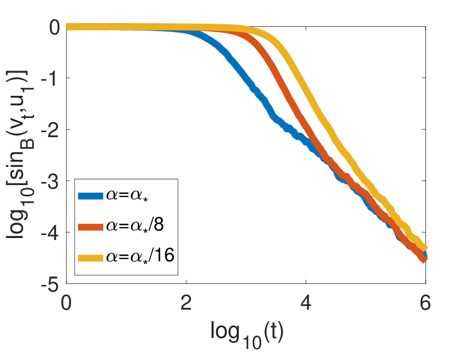
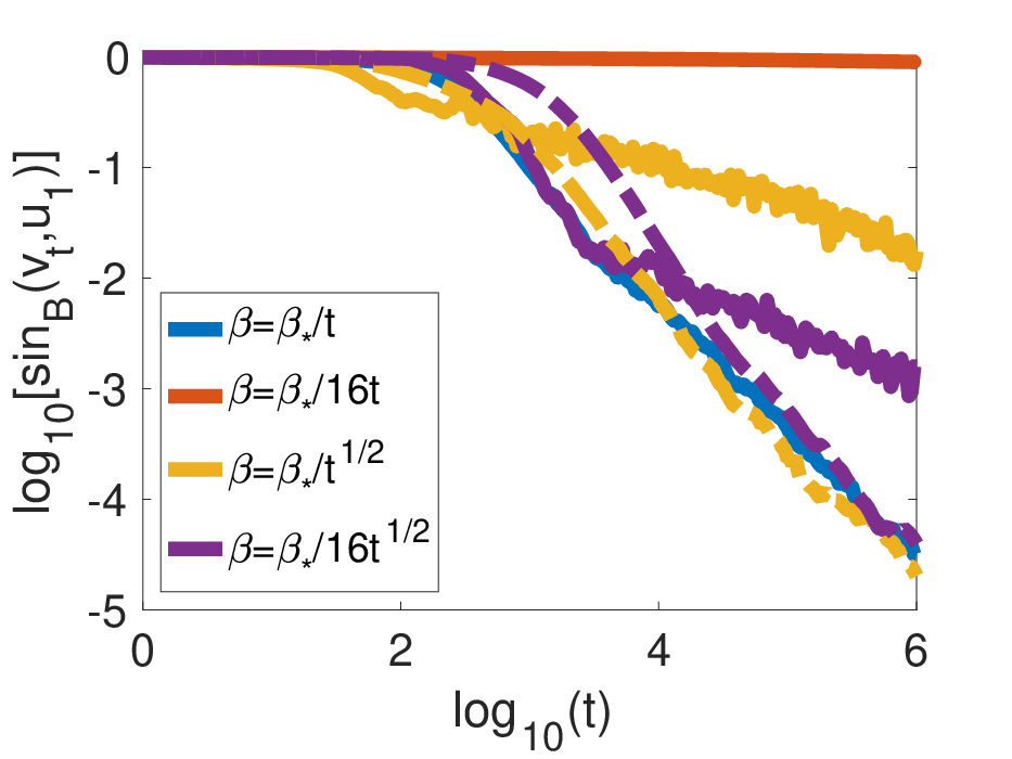
Figure 1: Synthetic Generalized Eigenvalue problem. Left: Comparison with two-steps methods. Middle: Robustness to step size αt\alpha_{t}. Right: Robustness to step size βt\beta_{t} (Streaming averaged Gen-Oja is dashed).

Here we illustrate the practical utility of Gen-Oja on a synthetic, streaming generalized eigenvector problem. We take d=20d=20 and T=106T=10^{6}. The streams (At,Bt)∈(ℝd×d)2(A_{t},B_{t})\in(\mathbb{R}^{d\times d})^{2} are normally-distributed with covariance matrix AA and BB with random eigenvectors and eigenvalues decaying as 1/i1/i, for i=1,…,di=1,\dots,d. Here R2R^{2} denotes the radius of the streams with R2=max⁡{Tr⁡A,Tr⁡B}R^{2}=\max\{\tr A,\tr B\}. All results are averaged over ten repetitions.

Comparison with two-steps methods.

In the left plot of Figure 1 we compare the behavior of Gen-Oja to different two-steps algorithms. Since the method by [4] is of complexity 𝒪⁡(d2)\mathcal{O}(d^{2}), we compare Gen-Oja to a method which alternates between one step of Oja’s algorithm and τ\tau steps of averaged stochastic gradient descent with constant step size 1/2​R21/2R^{2}. Gen-Oja is converging at rate 𝒪⁡(1/t)\mathcal{O}(1/t) whereas the other methods are very slow. For τ=10\tau=10, the solution of the inner loop is too inaccurate and the steps of Oja are inefficient. For τ=10000\tau=10000, the output of the sgd steps is very accurate but there are too few Oja iterations to make any progress. τ=1000\tau=1000 seems an optimal parameter choice but this method is slower than Gen-Oja by an order of magnitude.

Robustness to incorrect step-size α\alpha.

In the middle plot of Figure 1 we compare the behavior of Gen-Oja for step size α∈{α∗,α∗/8,α∗/16}\alpha\in\{\alpha_{*},\alpha_{*}/8,\alpha_{*}/16\} where α∗=1/R2\alpha_{*}=1/R^{2}. We observe that Gen-Oja converges at a rate 𝒪⁡(1/t)\mathcal{O}(1/t) independently of the choice of α\alpha.

Robustness to incorrect step-size βt\beta_{t}.

In the right plot of Figure 1 we compare the behavior of Gen-Oja for step size βt∈{β∗/t,β∗/16​t,β∗/i,β∗/16​i}\beta_{t}\in\{\beta_{*}/t,\beta_{*}/16t,\beta_{*}/\sqrt{i},\beta_{*}/16\sqrt{i}\} where β∗\beta_{*} corresponds to the minimal error after one pass over the data. We observe that Gen-Oja is not robust to the choice of the constant for step size βt∝1/t\beta_{t}\propto 1/t. If the constant is too small, the rate of convergence is arbitrary slow. We observe that considering the streaming average of [30] on Gen-Oja with a step size βt∝1/t\beta_{t}\propto 1/\sqrt{t} enables to recover the fast 𝒪⁡(1/t)\mathcal{O}(1/t) convergence while being robust to constant misspecification.

9 Conclusion

We have proposed and analyzed a simple online algorithm to solve the streaming generalized eigenvector problem and applied it to CCA. This algorithm, inspired by two-time-scale stochastic approximation achieves a fast 𝒪⁡(1/t)\mathcal{O}(1/t) convergence. Considering recovering the kk-principal generalized eigenvector (for k>1k>1) and obtaining a slow convergence rate 𝒪⁡(1/t)\mathcal{O}(1/\sqrt{t}) in the gap free setting are promising future directions. Finally, it would be worth considering removing the dimension dependence in our convergence guarantee.

Acknowledgements

We gratefully acknowledge the support of the NSF through grant IIS-1619362. AP acknowledges Huawei’s support through a BAIR-Huawei PhD Fellowship. This work was supported in part by the Mathematical Data Science program of the Office of Naval Research under grant number N00014-18-1-2764. This work was partially supported by AFOSR through grant FA9550-17-1-0308.

References

  • Allen-Zhu and Li [2017a] Z. Allen-Zhu and Y. Li. First efficient convergence for streaming k-PCA: a global, gap-free, and near-optimal rate. In Foundations of Computer Science (FOCS), 2017 IEEE 58th Annual Symposium on, pages 487–492. IEEE, 2017a.
  • Allen-Zhu and Li [2017b] Z. Allen-Zhu and Y. Li. Doubly accelerated methods for faster CCA and generalized eigendecomposition. In International Conference on Machine Learning, 2017b.
  • Andrieu et al. [2005] C. Andrieu, E. Moulines, and P. Priouret. Stability of stochastic approximation under verifiable conditions. SIAM Journal on Control and Optimization, 44(1):283–312, 2005.
  • Arora et al. [2017] R. Arora, T. V. Marinov, P. Mianjy, and N. Srebro. Stochastic approximation for canonical correlation analysis. In Advances in Neural Information Processing Systems. 2017.
  • Bach and Moulines [2013] F. Bach and E. Moulines. Non-strongly-convex smooth stochastic approximation with convergence rate O(1/n)(1/n). In Advances in Neural Information Processing Systems, 2013.
  • Benveniste et al. [1990] A. Benveniste, M. Métivier, and P. Priouret. Adaptive Algorithms and Stochastic Approximations. Springer Publishing Company, Incorporated, 1990.
  • Borkar [1997] V. S. Borkar. Stochastic approximation with two time scales. Systems & Control Letters, 29(5):291–294, 1997.
  • Borkar [2009] V. S. Borkar. Stochastic Approximation: A Dynamical Systems Viewpoint, volume 48. Springer, 2009.
  • Chaudhuri et al. [2009] K. Chaudhuri, S. M. Kakade, K. Livescu, and K. Sridharan. Multi-view clustering via canonical correlation analysis. In International Conference on Machine Learning, pages 129–136, 2009.
  • Diaconis and Freedman [1999] P. Diaconis and D. Freedman. Iterated random functions. SIAM Review, 41(1):45–76, 1999.
  • Dieuleveut et al. [2017] A. Dieuleveut, A. Durmus, and F. Bach. Bridging the gap between constant step size stochastic gradient descent and Markov chains. arXiv preprint arXiv:1707.06386, 2017.
  • Gao et al. [2017a] C. Gao, D. Garber, N. Srebro, J. Wang, and W. Wang. Stochastic canonical correlation analysis. arXiv preprint arXiv:1702.06533, 2017a.
  • Gao et al. [2017b] C. Gao, Z. Ma, and H. Zhou. Sparse CCA: Adaptive estimation and computational barriers. The Annals of Statistics, 45(5):2074–2101, 2017b.
  • Garber et al. [2016] D. Garber, E. Hazan, J. Jin, S. Kakade, C. Musco, P. Netrapalli, and A. Sidford. Faster eigenvector computation via shift-and-invert preconditioning. In International Conference on Machine Learning, 2016.
  • Ge et al. [2016] R. Ge, C. Jin, S. Kakade, P. Netrapalli, and A. Sidford. Efficient algorithms for large-scale generalized eigenvector computation and canonical correlation analysis. In International Conference on International Conference on Machine, 2016.
  • Hardt and Price [2014] M. Hardt and E. Price. The noisy power method: A meta algorithm with applications. In Advances in Neural Information Processing Systems, pages 2861–2869, 2014.
  • Hotelling [1936] H. Hotelling. Relations between two sets of variates. Biometrika, 28(3/4):321–377, 1936.
  • Jain et al. [2016] P. Jain, C. Jin, S. M. Kakade, P. Netrapalli, and A. Sidford. Streaming PCA: Matching matrix Bernstein and near-optimal finite sample guarantees for Oja’s algorithm. In Conference on Learning Theory, 2016.
  • Kakade and Foster [2007] S. M. Kakade and D. P. Foster. Multi-view regression via canonical correlation analysis. In International Conference on Computational Learning Theory, pages 82–96. Springer, 2007.
  • Karampatziakis and Mineiro [2013] N. Karampatziakis and P. Mineiro. Discriminative features via generalized eigenvectors. arXiv preprint arXiv:1310.1934, 2013.
  • Lu and Foster [2014] Y. Lu and D. P. Foster. Large scale canonical correlation analysis with iterative least squares. In Advances in Neural Information Processing Systems, 2014.
  • Ma et al. [2015] Z. Ma, Y. Lu, and D. Foster. Finding linear structure in large datasets with scalable canonical correlation analysis. In International Conference on International Conference on Machine Learning, 2015.
  • Meyn and Tweedie [2009] S. P. Meyn and R. L. Tweedie. Markov Chains and Stochastic Stability. Cambridge University Press, 2009.
  • Musco and Musco [2015] C. Musco and C. Musco. Randomized block Krylov methods for stronger and faster approximate singular value decomposition. In Advances in Neural Information Processing Systems, 2015.
  • Nemirovsky and Yudin [1983] A. S. Nemirovsky and D. B. Yudin. Problem Complexity and Method Efficiency in Optimization. Wiley-Interscience Series in Discrete Mathematics. John Wiley & Sons, 1983.
  • Oja [1982] E. Oja. Simplified neuron model as a principal component analyzer. Journal of Mathematical Biology, 15(3):267–273, 1982.
  • Robbins and Monro [1951] H. Robbins and S. Monro. A stochastic approximation method. The Annals of Mathematical Statistics, 22(3):400–407, 1951.
  • Shamir [2016] O. Shamir. Convergence of stochastic gradient descent for PCA. In International Conference on Machine Learning, 2016.
  • Steinsaltz [1999] D. Steinsaltz. Locally contractive iterated function systems. Annals of Probability, pages 1952–1979, 1999.
  • Tripuraneni et al. [2018] N. Tripuraneni, N. Flammarion, F. Bach, and M. I. Jordan. Averaging stochastic gradient descent on Riemannian manifolds. In Conference on Learning Theory, 2018.
  • Villani [2008] C. Villani. Optimal Transport: Old and New, volume 338. Springer-Verlag Berlin Heidelberg, 2008.
  • Wang et al. [2016] W. Wang, J. Wang, D. Garber, and N. Srebro. Efficient globally convergent stochastic optimization for canonical correlation analysis. In Advances in Neural Information Processing Systems, 2016.

Appendix A Proof of Lemma 2

We prove here the Lemma 2 which is an easy adaptation of [18, Lemma 3.1]. We first recall it.

Lemma 3.

Let H∈ℝd×dH\in\mathbb{R}^{d\times d}, (ui)i=1d(u_{i})_{i=1}^{d} and (u~i)i=1d(\tilde{u}_{i})_{i=1}^{d} the corresponding right and left eigenvectors of B−1​AB^{-1}A and w∈ℝdw\in\mathbb{R}^{d} chosen uniformly on the sphere, then with probability 1−δ1-\delta (over the randomness in the initial iterate)

sinB2⁡(ui,H​w)≤C​log⁡(1/δ)δ​Tr⁡(H​H⊤​∑j≠iu~j​u~j⊤)u~i⊤​H​H⊤​u~i,\sin^{2}_{B}(u_{i},Hw)\leq\frac{C\log(1/\delta)}{\delta}\frac{\tr(HH^{\top}\sum_{j\neq i}\tilde{u}_{j}\tilde{u}_{j}^{\top})}{\tilde{u}_{i}^{\top}HH^{\top}\tilde{u}_{i}},

for some universal constant C>0C>0.

Proof.

We follow the proof of [18]. Given a BB-normalized right eigenvector uiu_{i} of B−1​AB^{-1}A and w=g‖g‖2w=\frac{g}{\|g\|_{2}} for g∼𝒩⁡(0,I)g\sim\mathcal{N}(0,I), we consider:

sinB2⁡(ui,H​w)=1−OPEN(ui⊤​B​H​w)2)w⊤​H⊤​B​H​w=g⊤​H⊤​B1/2​[I−B1/2​ui​ui⊤​B1/2]​B1/2​H​gg⊤​H⊤​B​H​g.\sin^{2}_{B}(u_{i},Hw)=1-\frac{(u_{i}^{\top}BHw)^{2})}{w^{\top}H^{\top}BHw}=\frac{g^{\top}H^{\top}B^{1/2}\left[I-B^{1/2}u_{i}u_{i}^{\top}B^{1/2}\right]B^{1/2}Hg}{g^{\top}H^{\top}BHg}.

Moreover following Lemma 24 and denoting by u^i\hat{u}_{i} the corresponding orthonormal family of eigenvectors of the symmetric matrix B−1/2AB−1/2B^{-1/2}AB^{-1/2}, we have that ui=B−1/2u^iu_{i}=B^{-1/2}\hat{u}_{i}. This yields:

[I−B1/2​ui​ui⊤​B1/2]=[I−u^i​u^i⊤]=∑j≠iu^j​u^j⊤\left[I-B^{1/2}u_{i}u_{i}^{\top}B^{1/2}\right]=\left[I-\hat{u}_{i}\hat{u}_{i}^{\top}\right]=\sum_{j\neq i}\hat{u}_{j}\hat{u}_{j}^{\top}

Using now that the left eigenvectors of B−1​AB^{-1}A are given by u~i=B​ui\tilde{u}_{i}=Bu_{i}, we get

sinB2⁡(ui,H​w)=g⊤​H⊤​B1/2​[∑j≠iu^j​u^j⊤]​B1/2​H​gg⊤​H⊤​B​H​g=g⊤​H⊤​[∑j≠iu~j​u~j⊤]​H​gg⊤​H⊤​B​H​g.\sin^{2}_{B}(u_{i},Hw)=\frac{g^{\top}H^{\top}B^{1/2}\left[\sum_{j\neq i}\hat{u}_{j}\hat{u}_{j}^{\top}\right]B^{1/2}Hg}{g^{\top}H^{\top}BHg}=\frac{g^{\top}H^{\top}\left[\sum_{j\neq i}\tilde{u}_{j}\tilde{u}_{j}^{\top}\right]Hg}{g^{\top}H^{\top}BHg}.

We may bound the denominator by

g⊤​H⊤​B​H​g≥g⊤​H⊤​B1/2​u^i​u^i⊤​B1/2​H​g=g⊤​H⊤​u~i​u~i⊤​H​g=(u~i⊤​H​g)2≥δC1​u~i⊤​H​H⊤​u~i,g^{\top}H^{\top}BHg\geq g^{\top}H^{\top}B^{1/2}\hat{u}_{i}\hat{u}_{i}^{\top}B^{1/2}Hg=g^{\top}H^{\top}\tilde{u}_{i}\tilde{u}_{i}^{\top}Hg=(\tilde{u}_{i}^{\top}Hg)^{2}\geq\frac{\delta}{C_{1}}\tilde{u}_{i}^{\top}HH^{\top}\tilde{u}_{i},

where the last inequality follows as u~i⊤​H​g\tilde{u}_{i}^{\top}Hg is a Gaussian random vector with variance ‖H⊤​u~i‖22\|H^{\top}\tilde{u}_{i}\|_{2}^{2}. We can also bound the numerator as

g⊤​H⊤​[∑j≠iu~j​u~j⊤]​H​g≤C2​log⁡(1/δ)​Tr​[H⊤​∑j≠iu~j​u~j⊤​H],g^{\top}H^{\top}\left[\sum_{j\neq i}\tilde{u}_{j}\tilde{u}_{j}^{\top}\right]Hg\leq C_{2}\log(1/\delta)\tr[H^{\top}\sum_{j\neq i}\tilde{u}_{j}\tilde{u}_{j}^{\top}H],

since w⊤​H⊤​[∑j≠iu~j​u~j⊤]​H​ww^{\top}H^{\top}\left[\sum_{j\neq i}\tilde{u}_{j}\tilde{u}_{j}^{\top}\right]Hw is a χ2\chi^{2} random variable with Tr⁡[H⊤​∑j≠iu~j​u~j⊤​H]\tr[H^{\top}\sum_{j\neq i}\tilde{u}_{j}\tilde{u}_{j}^{\top}H] degrees of freedom. Therefore it exists a universal constant C>0C>0 such that

sinB2⁡(ui,H​w)≤C​log⁡(1/δ)δ​Tr⁡[H⊤​∑j≠iu~j​u~j⊤​H]u~i⊤​H​H⊤​u~i,\sin^{2}_{B}(u_{i},Hw)\leq C\frac{\log(1/\delta)}{\delta}\frac{\tr[H^{\top}\sum_{j\neq i}\tilde{u}_{j}\tilde{u}_{j}^{\top}H]}{\tilde{u}_{i}^{\top}HH^{\top}\tilde{u}_{i}},

with probability 1−δ1-\delta. ∎

Appendix B Deviation bounds for fast-mixing Markov Chain

In this section, we prove an upper bound on ‖𝔼⁡[ϵt+k|ℱt]‖2\|\mathbb{E}[\epsilon_{t+k}|\mathcal{F}_{t}]\|_{2}, where ϵt=(wt−B−1​A​wt−1)​vt−1⊤\epsilon_{t}=(w_{t}-B^{-1}Aw_{t-1})v_{t-1}^{\top} and ℱt=σ⁡(w0,⋯,wt)\mathcal{F}_{t}=\sigma(w_{0},\cdots,w_{t}) denotes the σ\sigma-algebra generated by w0,⋯,wtw_{0},\cdots,w_{t}. For the purpose of this section, we denote the pointwise upperbound on ‖wt‖2\|w_{t}\|_{2} by WtW_{t}. To begin with, we consider bounding the error term considering a fixed step-size αt=α\alpha_{t}=\alpha in order to keep the analysis cleaner. In Lemma 6, we bound the deviation of chains with step-size αt=O⁡(c/log⁡(d2​β+t))\alpha_{t}=O(c/\log(d^{2}\beta+t)) and fixed step size over a short horizon of length O⁡(log2⁡(1/βt))O(\log^{2}(1/\beta_{t}))

In order to prove the requisite bound, consider the following Markov chain given by,

θk+1=θk−η⁡[f′​(θ(k))+ϵk+1],\theta_{k+1}=\theta_{k}-\eta[f^{\prime}(\theta_{(k)})+\epsilon_{k+1}], (15)

where f:ℝd→ℝf:\mathbb{R}^{d}\rightarrow\mathbb{R} is some strongly convex function. We make use of the following proposition highlighting the fast-mixing property of constant step-size stochastic gradient descent from [11].

Proposition 1.

For any step size α∈(0,2/Lθ)\alpha\in(0,2/L_{\theta}), the markov chain given by (θk)k≥0(\theta_{k})_{k\geq 0} defined by recursion (15), admits a unique stationary distribution π∈𝒫⁡(ℝd)\pi\in\mathcal{P}(\mathbb{R}^{d}). In addition, for all θ∈ℝd,k∈ℕ\theta\in\mathbb{R}^{d},k\in\mathbb{N}, we have,

W22​(Rk​(θ,⋅),π)≤(1−2​μθ​η​(1−η​Lθ/2))k​∫ℝd‖θ−θ′‖22​𝑑π​(θ′),W_{2}^{2}(R^{k}(\theta,\cdot),\pi)\leq(1-2\mu_{\theta}\eta(1-\eta L_{\theta}/2))^{k}\int_{\mathbb{R}^{d}}\|\theta-\theta^{\prime}\|_{2}^{2}d\pi(\theta^{\prime}), (16)

where LθL_{\theta} and μθ\mu_{\theta} are the smoothness and the strong convexity parameters of ff respectively.

Now, consider the Markov chain given by

wtk+1=wtk−α⁡(Bk​wtk−Ak​vt),w_{t}^{k+1}=w_{t}^{k}-\alpha(B_{k}w_{t}^{k}-A_{k}v_{t}), (17)

where 𝔼⁡[Bk]=B,𝔼⁡[Ak]=A,wt0=wt\mathbb{E}[B_{k}]=B,\mathbb{E}[A_{k}]=A,w_{t}^{0}=w_{t} where wtw_{t} is as given by Algorithm 1. Equation (17) represents the update step for the kt​hk^{th} step of a Markov chain starting at wtw_{t} and performing stochastic gradient updates on ft​(w)=1/2​w⊤​B​w−w⊤​A​vtf_{t}(w)=1/2w^{\top}Bw-w^{\top}Av_{t}.

For this function ftf_{t}, the smoothness constant L=λBL=\lambda_{B}. Further, proposition 1 guarantees the existence of a unique stationary distribution π\pi and we have that under the stationary distribution,

𝔼π​[wtk]=B−1​A​vt.\mathbb{E}_{\pi}[w_{t}^{k}]=B^{-1}Av_{t}. (18)
Lemma 4.

For the Markov chain given by (17) with any step size α∈(0,2/λB)\alpha\in(0,2/\lambda_{B}), for any k>log⁡(λ1ϵ)μ​α​(1−α​λB2){k>\frac{\log(\frac{\lambda_{1}}{\epsilon})}{\mu\alpha\left(1-\frac{\alpha\lambda_{B}}{2}\right)}}, we have

∥𝔼[wtk−B−1Avt]|ℱt∥22≤ϵ\|\mathbb{E}[w_{t}^{k}-B^{-1}Av_{t}]|\mathcal{F}_{t}\|_{2}^{2}\leq\epsilon
Proof.

We know from (18), B−1​A​vt=𝔼π​[wtk]B^{-1}Av_{t}=\mathbb{E}_{\pi}[w_{t}^{k}]. Now, we consider the term ∥𝔼[wtk−B−1Avt]|ℱt∥22\|\mathbb{E}[w_{t}^{k}-B^{-1}Av_{t}]|\mathcal{F}_{t}\|_{2}^{2},

∥𝔼[wtk−B−1Avt]|ℱt∥22\displaystyle\|\mathbb{E}[w_{t}^{k}-B^{-1}Av_{t}]|\mathcal{F}_{t}\|_{2}^{2} =∥𝔼[wtk]−𝔼π[w]|ℱt∥22\displaystyle=\|\mathbb{E}[w_{t}^{k}]-\mathbb{E}_{\pi}[w]|\mathcal{F}_{t}\|_{2}^{2}
=∥𝔼Γ⁡(Rk​(wt,⋅),π)[wtk−w]|∥22\displaystyle=\|\mathbb{E}_{\Gamma(R^{k}(w_{t},\cdot),\pi)}[w_{t}^{k}-w]|\|_{2}^{2}
≤ζ1𝔼Γ⁡(Rk​(wt,⋅),π)​[‖wtk−w‖22]\displaystyle\stackrel{{\scriptstyle\zeta_{1}}}{{\leq}}\mathbb{E}_{\Gamma(R^{k}(w_{t},\cdot),\pi)}[\|w_{t}^{k}-w\|_{2}^{2}]
=ζ2W22​(Rk​(wt,⋅),π)\displaystyle\stackrel{{\scriptstyle\zeta_{2}}}{{=}}W_{2}^{2}(R^{k}(w_{t},\cdot),\pi)
≤ζ3(1−2​μ​α​(1−α​λB/2))k​λ12,\displaystyle\stackrel{{\scriptstyle\zeta_{3}}}{{\leq}}(1-2\mu\alpha(1-\alpha\lambda_{B}/2))^{k}\lambda_{1}^{2},

where Rk​(wt,⋅)R^{k}(w_{t},\cdot) denotes the kk-step transition kernel of the Markov chain beginning from wtw_{t}, Γ⁡(Rk​(wt,⋅),π)\Gamma(R^{k}(w_{t},\cdot),\pi) denotes any coupling of the distributions Rk​(wt,⋅)R^{k}(w_{t},\cdot) and π\pi and 𝔼Γ⁡(⋅,⋅)\mathbb{E}_{\Gamma(\cdot,\cdot)} denotes the expectation under the joint distribution, conditioned on ℱt\mathcal{F}_{t}. Now, ζ1\zeta_{1} follows from Jenson’s inequality, ζ2\zeta_{2} follows by setting Γ⁡(Rk​(wt,⋅),π)\Gamma(R^{k}(w_{t},\cdot),\pi) to the coupling attaining the infimum in the wasserstein bound and ζ3\zeta_{3} follows by using proposition (1). The lemma now follows by setting k>log⁡(λ1ϵ)μ​α​(1−α​λB2){k>\frac{\log(\frac{\lambda_{1}}{\epsilon})}{\mu\alpha\left(1-\frac{\alpha\lambda_{B}}{2}\right)}}. [see, e.g., 31, for more properties of W2W_{2}] ∎

Deviation bound for ‖vt−vt+k‖2\|v_{t}-v_{t+k}\|_{2}: We now bound the deviation of vt+kv_{t+k} from vtv_{t} if we execute kk steps of the algorithm sarting from vtv_{t},

‖vt−vt+k‖2≤∑i=0k−1‖vt+i−vt+i+1‖2.\|v_{t}-v_{t+k}\|_{2}\leq\sum_{i=0}^{k-1}\|v_{t+i}-v_{t+i+1}\|_{2}. (19)

Now, for a single step of the algorithm, using the contractivity of the projection

‖vi−vi+1‖2≤‖vi−vi+1′‖vi+1′‖‖2≤‖vi−vi+1′‖2≤Wi+1​βi+1.\|v_{i}-v_{i+1}\|_{2}\leq\|v_{i}-\frac{v_{i+1}^{\prime}}{\|v_{i+1}^{\prime}\|}\|_{2}\leq\|v_{i}-v_{i+1}^{\prime}\|_{2}\leq W_{i+1}\beta_{i+1}.

Using the above bound in (19), we obtain,

‖vt−vt+k‖2≤Wt+k​∑i=0k−1βt+i+1≤Wt+k​k​βt,\|v_{t}-v_{t+k}\|_{2}\leq W_{t+k}\sum_{i=0}^{k-1}\beta_{t+i+1}\leq W_{t+k}k\beta_{t}, (20)

by using the fact that βt\beta_{t} is a decreasing sequence.

Deviation bound for Coupled Chains: Consider the sequence (wt+i)i=0k(w_{t+i})_{i=0}^{k} as generated by Algorithm 1, assuming a constant step-size α\alpha, and the sequence (wti)i=1k(w_{t}^{i})_{i=1}^{k} generated by the recurrence (17) in the case when both have the same randomness with respect to the sampling of the matrices At+i,Bt+iA_{t+i},B_{t+i}. We now obtain a bound on ∥𝔼[wtk−wt+k]|ℱt∥2{\|\mathbb{E}[w_{t}^{k}-w_{t+k}]|\mathcal{F}_{t}\|_{2}}.

∥𝔼[wtk−wt+k]|ℱt∥2=∥𝔼[𝔼[(I−αBt+k)(wtk−1−wt+k−1)−αAt+k(vt−vt+k−1)]|ℱt+k−1]|ℱt∥2=∥𝔼[(I−αB)(wtk−1−wt+k−1)−αA(vt−vt+k−1)]|ℱt∥2=α​‖𝔼⁡[∑i=0k−1(I−α​B)i​A​(vt−vt+k−1−i)|ℱt]‖2≤α​𝔼​[∑i=0k−1‖(I−α​B)i​A​(vt−vt+k−1−i)‖2|ℱt]≤α​λA​Wt+k​k​∑i=0k−1(1−α​μ)i​βt+k−1−i≤λA​Wt+k​k​βtμ,\displaystyle\begin{split}\|\mathbb{E}[w_{t}^{k}-w_{t+k}]|\mathcal{F}_{t}\|_{2}&=\|\mathbb{E}\left[\mathbb{E}[(I-\alpha B_{t+k})(w_{t}^{k-1}-w_{t+k-1})-\alpha A_{t+k}(v_{t}-v_{t+k-1})\right]|\mathcal{F}_{t+k-1}]|\mathcal{F}_{t}\|_{2}\\ &=\|\mathbb{E}\left[(I-\alpha B)(w_{t}^{k-1}-w_{t+k-1})-\alpha A(v_{t}-v_{t+k-1})\right]|\mathcal{F}_{t}\|_{2}\\ &\vdots\\ &=\alpha\left\|\mathbb{E}\left[\sum_{i=0}^{k-1}(I-\alpha B)^{i}A(v_{t}-v_{t+k-1-i})|\mathcal{F}_{t}\right]\right\|_{2}\\ &\leq\alpha\mathbb{E}\left[\sum_{i=0}^{k-1}\left\|(I-\alpha B)^{i}A(v_{t}-v_{t+k-1-i})\right\|_{2}|\mathcal{F}_{t}\right]\\ &\leq\alpha\lambda_{A}W_{t+k}k\sum_{i=0}^{k-1}\left(1-\alpha\mu\right)^{i}\beta_{t+k-1-i}\\ &\leq\frac{\lambda_{A}W_{t+k}k\beta_{t}}{\mu},\end{split} (21)

where we expand the terms using the recursion and bound the geometric series by using that α​μ≤1\alpha\mu\leq 1.

Lemma 5.

For any choice of k>log⁡(1βt)2​μ​α​(1−α​λB2){k>\frac{\log(\frac{1}{\beta_{t}})}{2\mu\alpha\left(1-\frac{\alpha\lambda_{B}}{2}\right)}}, we have that

‖𝔼⁡[ϵt+k|ℱt]‖2≤(λA​Wt+k​kμ+λ1​(1+2​Wt+k​k)+Wt+k2​k)​βt=O⁡(Wt+k2​k​βt)\|\mathbb{E}[\epsilon_{t+k}|\mathcal{F}_{t}]\|_{2}\leq\left(\frac{\lambda_{A}W_{t+k}k}{\mu}+\lambda_{1}(1+2W_{t+k}k)+W_{t+k}^{2}k\right)\beta_{t}=O(W_{t+k}^{2}k\beta_{t})
Proof.

Consider the term ‖𝔼⁡[ϵt+k|ℱt]‖2\|\mathbb{E}[\epsilon_{t+k}|\mathcal{F}_{t}]\|_{2},

‖𝔼⁡[ϵt+k|ℱt]‖2\displaystyle\|\mathbb{E}[\epsilon_{t+k}|\mathcal{F}_{t}]\|_{2} =‖𝔼⁡[(wt+k−B−1​A​vt+k−1)​vt+k−1⊤|ℱt]‖2\displaystyle=\|\mathbb{E}[(w_{t+k}-B^{-1}Av_{t+k-1})v_{t+k-1}^{\top}|\mathcal{F}_{t}]\|_{2}
≤‖𝔼⁡[(wt+k−B−1​A​vt+k−1)​vt⊤|ℱt]‖2⏟(I)+|𝔼[(wt+k−B−1Avt+k−1)(vt+k−1−vt)⊤|ℱt]∥2⏟(I​I).\displaystyle\leq\underbrace{\|\mathbb{E}[(w_{t+k}-B^{-1}Av_{t+k-1})v_{t}^{\top}|\mathcal{F}_{t}]\|_{2}}_{(I)}+\|\underbrace{\mathbb{E}[(w_{t+k}-B^{-1}Av_{t+k-1})(v_{t+k-1}-v_{t})^{\top}|\mathcal{F}_{t}]\|_{2}}_{(II)}.

We first analyze term (I) in the expansion above.

‖𝔼⁡[(wt+k−B−1​A​vt+k−1)​vt⊤|ℱt]‖2\displaystyle\|\mathbb{E}[(w_{t+k}-B^{-1}Av_{t+k-1})v_{t}^{\top}|\mathcal{F}_{t}]\|_{2} =∥𝔼[(wt+k−wtk)+(wtk−B−1Avt)\displaystyle=\|\mathbb{E}[(w_{t+k}-w_{t}^{k})+(w_{t}^{k}-B^{-1}Av_{t})
+(B−1Avt−B−1Avt+k−1))vt⊤|ℱt]∥2\displaystyle\qquad+(B^{-1}Av_{t}-B^{-1}Av_{t+k-1}))v_{t}^{\top}|\mathcal{F}_{t}]\|_{2}
≤∥𝔼[(wt+k−wtk)|ℱt]vt⊤∥2+∥𝔼[(wtk−B−1Avt+k−1))|ℱt]vt⊤∥2\displaystyle\leq\|\mathbb{E}[(w_{t+k}-w_{t}^{k})|\mathcal{F}_{t}]v_{t}^{\top}\|_{2}+\|\mathbb{E}[(w_{t}^{k}-B^{-1}Av_{t+k-1}))|\mathcal{F}_{t}]v_{t}^{\top}\|_{2}
≤∥𝔼[(wt+k−wtk)|ℱt]∥2+∥𝔼[(wtk−B−1Avt))|ℱt]∥2\displaystyle\leq\|\mathbb{E}[(w_{t+k}-w_{t}^{k})|\mathcal{F}_{t}]\|_{2}+\|\mathbb{E}[(w_{t}^{k}-B^{-1}Av_{t}))|\mathcal{F}_{t}]\|_{2}
+|𝔼[(B−1Avt−B−1Avt+k−1))|ℱt]∥2\displaystyle\quad+|\mathbb{E}[(B^{-1}Av_{t}-B^{-1}Av_{t+k-1}))|\mathcal{F}_{t}]\|_{2}
≤ζ1λA​Wt+k​kμ​βt+λ1​βt+λ1​Wt+k​k​βt\displaystyle\stackrel{{\scriptstyle\zeta_{1}}}{{\leq}}\frac{\lambda_{A}W_{t+k}k}{\mu}\beta_{t}+\lambda_{1}\beta_{t}+\lambda_{1}W_{t+k}k\beta_{t}
=(λA​Wt+k​kμ+λ1​(1+Wt+k​k))​βt,\displaystyle=(\frac{\lambda_{A}W_{t+k}k}{\mu}+\lambda_{1}(1+W_{t+k}k))\beta_{t}, (22)

where ζ1\zeta_{1} follows from using lemma 4 with k>log⁡(1βt)2​μ​α​(1−α​λB2){k>\frac{\log(\frac{1}{\beta_{t}})}{2\mu\alpha\left(1-\frac{\alpha\lambda_{B}}{2}\right)}}, bound in (20) and bound in (21).

We now look at term (II) in the expansion.

‖𝔼⁡[(wt+k−B−1​A​vt+k−1)​(vt+k−1−vt)⊤|ℱt]‖2\displaystyle\|\mathbb{E}[(w_{t+k}-B^{-1}Av_{t+k-1})(v_{t+k-1}-v_{t})^{\top}|\mathcal{F}_{t}]\|_{2} ≤(Wt+k+λ1)​‖vt+k−1−vt‖\displaystyle\leq(W_{t+k}+\lambda_{1})\|v_{t+k-1}-v_{t}\|
≤Wt+k​(Wt+k+λ1)​k​βt.\displaystyle\leq W_{t+k}(W_{t+k}+\lambda_{1})k\beta_{t}. (23)

Combininig the bounds in (22) and (23), we get the desired result. ∎

The bound we proved above hold for any fixed fixed step-size α\alpha. However, in order to obtain the sharpest convergence result for our algorithm, we would require the step size αt=clog⁡(d2​β+t)\alpha_{t}=\frac{c}{\log(d^{2}\beta+t)} for some constant β\beta. We provide the following lemma which accomodates for this change.

In order to get a bound on the noise term with a logarithmically decaying step size, in addition to the previous analysis, we consider processes (w^t+i)i=1k(\hat{w}_{t+i})_{i=1}^{k} and (v^t+i)i=1k(\hat{v}_{t+i})_{i=1}^{k} which evolve with the same random matrices At+iA_{t+i} and Bt+iB_{t+i}, but with a step size of αt+i=αt=clog⁡(d2​β+t)\alpha_{t+i}=\alpha_{t}=\frac{c}{\log(d^{2}\beta+t)}.

Pointwise bound on ‖w^t+k‖2\|\hat{w}_{t+k}\|_{2}: We can obtain a pointwise bound on ‖w^t+k‖2\|\hat{w}_{t+k}\|_{2} using the simple recursive evaluation:

‖w^t+k‖\displaystyle\|\hat{w}_{t+k}\| ≤‖I−αt​Bt+k‖2​‖w^t+k−1‖2+αt​λA\displaystyle\leq\|I-\alpha_{t}B_{t+k}\|_{2}\|\hat{w}_{t+k-1}\|_{2}+\alpha_{t}\lambda_{A}
≤Wt+k​αt​λA,\displaystyle\leq W_{t}+k\alpha_{t}\lambda_{A}, (24)

where the final inequality follows from recursing on ‖w^t+k−1‖\|\hat{w}_{t+k-1}\| and using the assumption that Bi⪰0B_{i}\succeq 0.

Deviation bound for ‖vt+k−v^t+k‖2\|v_{t+k}-\hat{v}_{t+k}\|_{2}: We can obtain a bound on this quantity as follows:

‖vt+k−v^t+k‖2\displaystyle\|v_{t+k}-\hat{v}_{t+k}\|_{2} ≤‖vt+k−vt+k′‖2+‖v^t+k′−v^t+k‖2+‖vt+k′−v^t+k′‖2\displaystyle\leq\|v_{t+k}-v^{\prime}_{t+k}\|_{2}+\|\hat{v}_{t+k}^{\prime}-\hat{v}_{t+k}\|_{2}+\|v^{\prime}_{t+k}-\hat{v}_{t+k}^{\prime}\|_{2}
≤2​βt+k​Wt+k+2​βt+k​‖w^t+k‖2+‖βt+k​(wt+k−w^t+k)‖2+‖vt+k−1−v^t+k−1‖2\displaystyle\leq 2\beta_{t+k}W_{t+k}+2\beta_{t+k}\|\hat{w}_{t+k}\|_{2}+\|\beta_{t+k}(w_{t+k}-\hat{w}_{t+k})\|_{2}+\|v_{t+k-1}-\hat{v}_{t+k-1}\|_{2}
≤2​(∑i=1kβt+i​(Wt+i+‖w^t+i‖2))+∑i=1kβt+i​‖wt+i−w^t+i‖2\displaystyle\leq 2\left(\sum_{i=1}^{k}\beta_{t+i}(W_{t+i}+\|\hat{w}_{t+i}\|_{2})\right)+\sum_{i=1}^{k}\beta_{t+i}\|w_{t+i}-\hat{w}_{t+i}\|_{2}
≤3​βt​k​(2​Wt+k+k​αt​λA),\displaystyle\leq 3\beta_{t}k(2W_{t+k}+k\alpha_{t}\lambda_{A}), (25)

where the final bound is obtained using ‖wt+k‖2≤Wt+k\|w_{t+k}\|_{2}\leq W_{t+k} and ‖w^t+k‖2≤Wt+k+k​αt​λA\|\hat{w}_{t+k}\|_{2}\leq W_{t+k}+k\alpha_{t}\lambda_{A} from Equation (24)

Lemma 6.

For any choice of k>log⁡(1βt)2​μ​αt​(1−αt​λB2){k>\frac{\log(\frac{1}{\beta_{t}})}{2\mu\alpha_{t}\left(1-\frac{\alpha_{t}\lambda_{B}}{2}\right)}} and αt∈(0,2/λB)\alpha_{t}\in(0,2/\lambda_{B}) of the form αt=clog⁡(d2​β+t)\alpha_{t}=\frac{c}{\log(d^{2}\beta+t)}, we have that

‖𝔼⁡[ϵt+k|ℱt]‖2\displaystyle\|\mathbb{E}[\epsilon_{t+k}|\mathcal{F}_{t}]\|_{2} ≤(λA​Wt+k​kμ+λ1​(1+2​Wt+k​k)+Wt+k2​k)​βt\displaystyle\leq\left(\frac{\lambda_{A}W_{t+k}k}{\mu}+\lambda_{1}(1+2W_{t+k}k)+W_{t+k}^{2}k\right)\beta_{t}
+λB​Wt+k​k​αt​βtc​μ​γ+λA​k​αt​βtc​μ​γ+3​λA​βt​k​(2​Wt+k+k​αt​λA)μ\displaystyle\quad+\frac{\lambda_{B}W_{t+k}k\alpha_{t}\beta_{t}}{c\mu\gamma}+\frac{\lambda_{A}k\alpha_{t}\beta_{t}}{c\mu\gamma}+\frac{3\lambda_{A}\beta_{t}k(2W_{t+k}+k\alpha_{t}\lambda_{A})}{\mu}
+(2​Wt+k+k​αt​λA)​Wt+k​k​βt.\displaystyle\quad+(2W_{t+k}+k\alpha_{t}\lambda_{A})W_{t+k}k\beta_{t}.

In other words, we get that ‖𝔼⁡[ϵt+k|ℱt]‖2=O⁡(βt​k2​αt​Wt+k)\|\mathbb{E}[\epsilon_{t+k}|\mathcal{F}_{t}]\|_{2}=O(\beta_{t}k^{2}\alpha_{t}W_{t+k}).

Proof.

In continuation from Lemma 5, we consider bounding the deviation of the process w^t+k\hat{w}_{t+k} from the process wt+kw_{t+k}. The extra components in the error term ϵt\epsilon_{t} remain the same and we ignore them for clarity of this lemma.

‖𝔼⁡[(wt+k−w^t+k)​vt+k−1⊤|ℱt]‖2≤‖𝔼⁡[(wt+k−w^t+k)​vt⊤|ℱt]‖2⏟(I)+‖𝔼⁡[(wt+k−w^t+k)​(vt+k−1−vt)⊤|ℱt]‖2⏟(II)\|\mathbb{E}[(w_{t+k}-\hat{w}_{t+k})v_{t+k-1}^{\top}|\mathcal{F}_{t}]\|_{2}\leq\underbrace{\|\mathbb{E}[(w_{t+k}-\hat{w}_{t+k})v_{t}^{\top}|\mathcal{F}_{t}]\|_{2}}_{\text{(I)}}+\underbrace{\|\mathbb{E}[(w_{t+k}-\hat{w}_{t+k})(v_{t+k-1}-v_{t})^{\top}|\mathcal{F}_{t}]\|_{2}}_{\text{(II)}} (26)

We proceed by first analyzing term (I) in Equation (26).

‖𝔼⁡[(wt+k−w^t+k)​vt⊤|ℱt]‖2\displaystyle\|\mathbb{E}[(w_{t+k}-\hat{w}_{t+k})v_{t}^{\top}|\mathcal{F}_{t}]\|_{2} =∥𝔼[𝔼[((I−αt+kBt+k)wt+k−1+αt+kAt+kvt+k−1)\displaystyle=\|\mathbb{E}[\mathbb{E}[((I-\alpha_{t+k}B_{t+k})w_{t+k-1}+\alpha_{t+k}A_{t+k}v_{t+k-1})
−((I−αtBt+k)w^t+k−1+αtAt+kv^t+k−1)|ℱt+k−1]vt⊤|ℱt]∥2\displaystyle\quad-((I-\alpha_{t}B_{t+k})\hat{w}_{t+k-1}+\alpha_{t}A_{t+k}\hat{v}_{t+k-1})|\mathcal{F}_{t+k-1}]v_{t}^{\top}|\mathcal{F}_{t}]\|_{2}
=∥𝔼[((I−αt+kB)wt+k−1+αt+kAvt+k−1)\displaystyle=\|\mathbb{E}[((I-\alpha_{t+k}B)w_{t+k-1}+\alpha_{t+k}Av_{t+k-1})
−((I−αtB)w^t+k−1+αtAv^t+k−1)|ℱt]vt⊤∥2\displaystyle\qquad-((I-\alpha_{t}B)\hat{w}_{t+k-1}+\alpha_{t}A\hat{v}_{t+k-1})|\mathcal{F}_{t}]v_{t}^{\top}\|_{2}
=∥𝔼[(αt−αt+k)Bwt+k−1+(I−αtB)(wt+k−1−w^t+k−1)\displaystyle=\|\mathbb{E}[(\alpha_{t}-\alpha_{t+k})Bw_{t+k-1}+(I-\alpha_{t}B)(w_{t+k-1}-\hat{w}_{t+k-1})
+(αt+k−αt)Avt+k−1+αtA(vt+k−1−v^t+k−1))|ℱt]vt⊤∥2\displaystyle\quad+(\alpha_{t+k}-\alpha_{t})Av_{t+k-1}+\alpha_{t}A(v_{t+k-1}-\hat{v}_{t+k-1}))|\mathcal{F}_{t}]v_{t}^{\top}\|_{2}
≤‖𝔼⁡[∑i=1k(αt−αt+i)​(I−αt​B)k−i​B​wt+i−1|ℱt]​vt⊤‖2\displaystyle\leq\left\|\mathbb{E}\left[\sum_{i=1}^{k}(\alpha_{t}-\alpha_{t+i})(I-\alpha_{t}B)^{k-i}Bw_{t+i-1}|\mathcal{F}_{t}\right]v_{t}^{\top}\right\|_{2}
+‖𝔼⁡[∑i=1k(αt+i−αt)​(I−αt​B)k−i​A​vt+i−1|ℱt]​vt⊤‖2\displaystyle\quad+\left\|\mathbb{E}\left[\sum_{i=1}^{k}(\alpha_{t+i}-\alpha_{t})(I-\alpha_{t}B)^{k-i}Av_{t+i-1}|\mathcal{F}_{t}\right]v_{t}^{\top}\right\|_{2}
+αt​‖𝔼⁡[∑i=1k(I−αt​B)k−i​A​(vt+i−1−v^t+i−1)|ℱt]​vt⊤‖2\displaystyle\quad+\alpha_{t}\left\|\mathbb{E}\left[\sum_{i=1}^{k}(I-\alpha_{t}B)^{k-i}A(v_{t+i-1}-\hat{v}_{t+i-1})|\mathcal{F}_{t}\right]v_{t}^{\top}\right\|_{2}
≤(αt−αt+k)​λB​Wt+kαt​μ+(αt−αt+k)​λAαt​μ+λA​‖vt+k−1−v^t+k−1‖2μ\displaystyle\leq\frac{(\alpha_{t}-\alpha_{t+k})\lambda_{B}W_{t+k}}{\alpha_{t}\mu}+\frac{(\alpha_{t}-\alpha_{t+k})\lambda_{A}}{\alpha_{t}\mu}+\frac{\lambda_{A}\|v_{t+k-1}-\hat{v}_{t+k-1}\|_{2}}{\mu}
≤λB​Wt+k​k​αtc​μ​(d​β+t)+λA​k​αtc​μ​(d​β+t)+3​λA​βt​k​(2​Wt+k+k​αt​λA)μ\displaystyle\leq\frac{\lambda_{B}W_{t+k}k\alpha_{t}}{c\mu(d\beta+t)}+\frac{\lambda_{A}k\alpha_{t}}{c\mu(d\beta+t)}+\frac{3\lambda_{A}\beta_{t}k(2W_{t+k}+k\alpha_{t}\lambda_{A})}{\mu}
≤λB​Wt+k​k​αt​βtc​μ​b+λA​k​αt​βtc​μ​b+3​λA​βt​k​(2​Wt+k+k​αt​λA)μ\displaystyle\leq\frac{\lambda_{B}W_{t+k}k\alpha_{t}\beta_{t}}{c\mu b}+\frac{\lambda_{A}k\alpha_{t}\beta_{t}}{c\mu b}+\frac{3\lambda_{A}\beta_{t}k(2W_{t+k}+k\alpha_{t}\lambda_{A})}{\mu} (27)

where the second last inequality follows using Jensen’s ineuality along with a trinagle inequality and using the fact that B⪰μ​IB\succeq\mu I and the last equality follows from using the form of βt=bd2​β+t\beta_{t}=\frac{b}{d^{2}\beta+t} for some constant bb.

We now consider term (II) in Equation (26).

‖𝔼⁡[(wt+k−w^t+k)​(vt+k−1−vt)⊤|ℱt]‖2≤(2​Wt+k+k​αt​λA)​Wt+k​k​βt,\displaystyle\|\mathbb{E}[(w_{t+k}-\hat{w}_{t+k})(v_{t+k-1}-v_{t})^{\top}|\mathcal{F}_{t}]\|_{2}\leq(2W_{t+k}+k\alpha_{t}\lambda_{A})W_{t+k}k\beta_{t}, (28)

by using Jensen’s inequality along with bound (20). Combining (27) and (28) with (26), and using Lemma 5, we obtain the desired result. ∎

Note that in order to prove the final convergence for Algorithm 1, we use the form of the step sizes αt\alpha_{t} and βt\beta_{t} as mentioned in this section.

In the following sections we denote by rt=12​μ​αt​(1−αt​λB2)​log2⁡(1βt){r_{t}=\frac{1}{2\mu\alpha_{t}\left(1-\frac{\alpha_{t}\lambda_{B}}{2}\right)}}\log^{2}(\frac{1}{\beta_{t}}) and 𝒜t\mathcal{A}_{t} to be such that:

𝒜t​rt​βt≥‖𝔼⁡[ϵt+k|ℱt]‖\mathcal{A}_{t}r_{t}\beta_{t}\geq\|\mathbb{E}\left[\epsilon_{t+k}|\mathcal{F}_{t}\right]\| (29)

When αt=clog⁡(d2​β+t)\alpha_{t}=\frac{c}{\log(d^{2}\beta+t)}, rtr_{t} will be O⁡(log3⁡(1/βt))O(\log^{3}(1/\beta_{t})) and when αt\alpha_{t} is contant, rtr_{t} will be O⁡(log2⁡(1/βt))O(\log^{2}(1/\beta_{t})).

Appendix C Controlling Markov Chain wtw_{t}

For the purpose of this section, we stick with bounds RA,RBR_{A},R_{B} the maximum of which equals RR in the main paper. In this section we provide a bound on the norm of the markov chain wtw_{t}. We start by showing the pp moments of the norms of wtw_{t} are bounded as long as αt=α\alpha_{t}=\alpha a small enough constant ∀t\forall t. Ultimately we will use a time dependent αt\alpha_{t} as defined in the previous section, but for warm up we start by showing some lemmas that bring out the behavior of wtw_{t} when αt=α\alpha_{t}=\alpha for all tt. The proofs for a moving αt\alpha_{t} will follow a similar though technically involved arguments.

Lemma 7.

For α≤1/RB2\alpha\leq 1/R_{B}^{2} we have

𝔼⁡[‖wt‖22]≤[(1−μ​α/2)t​‖w0‖2+2​RA2μ]2.\mathbb{E}[\|w_{t}\|_{2}^{2}]\leq\big[(1-\mu\alpha/2)^{t}\|w_{0}\|_{2}+2\frac{R_{A}^{2}}{\mu}\big]^{2}.

If, in addition we assume that α≤2RB2​(p−2)\alpha\leq\frac{2}{R_{B}^{2}(p-2)} for p≥3p\geq 3 we have:

𝔼⁡[‖wt‖2p]≤[(1−μ​α/4)t​‖w0‖2+4​RA2μ]p.\mathbb{E}\big[\|w_{t}\|_{2}^{p}\big]\leq\Big[(1-\mu\alpha/4)^{t}\|w_{0}\|_{2}+4\frac{R_{A}^{2}}{\mu}\Big]^{p}.
Proof.

We first expand wt+1=(I−α​Bt+1)​wt+α​At+1​vtw_{t+1}=(I-\alpha B_{t+1})w_{t}+\alpha A_{t+1}v_{t} and use the Minkowski inequality on L2L_{2}-norm (denoted by ∥∥L2\|\|_{L_{2}}) to obtain:

‖wt+1‖L2≤‖(I−α​Bt)​wt‖L2+‖α​At+1​vt‖L2\|w_{t+1}\|_{L_{2}}\leq\|(I-\alpha B_{t})w_{t}\|_{L_{2}}+\|\alpha A_{t+1}v_{t}\|_{L_{2}}

We directly have that ‖α​At+1​vt‖L2≤α​RA2\|\alpha A_{t+1}v_{t}\|_{L_{2}}\leq\alpha R_{A}^{2} almost surely and we can directly compute for α<1/RB2\alpha<1/R^{2}_{B}:

‖(I−α​Bt+1)​wt‖L22\displaystyle\|(I-\alpha B_{t+1})w_{t}\|_{L_{2}}^{2} =\displaystyle= 𝔼⁡[wt⊤​(I−α​Bt+1)2​wt]=𝔼⁡[wt⊤​(I−2​α​Bt+1+α2​Bt+12)​wt]\displaystyle\mathbb{E}[w_{t}^{\top}(I-\alpha B_{t+1})^{2}w_{t}]=\mathbb{E}[w_{t}^{\top}(I-2\alpha B_{t+1}+\alpha^{2}B_{t+1}^{2})w_{t}]
≤(1)\displaystyle\overset{(1)}{\leq} 𝔼⁡[wt⊤​(I−α​Bt+1)​wt]≤𝔼⁡[wt⊤​(I−α​𝔼​[Bt+1|ℱ𝓉])​wt]≤(1−α​μ)​𝔼​[‖wt‖22],\displaystyle\mathbb{E}[w_{t}^{\top}(I-\alpha B_{t+1})w_{t}]\leq\mathbb{E}[w_{t}^{\top}(I-\alpha\mathbb{E}[B_{t+1}|\mathcal{F_{t}}])w_{t}]\leq(1-\alpha\mu)\mathbb{E}[\|w_{t}\|_{2}^{2}],

where (1)(1) follows as Bt+1≼RB2​IB_{t+1}\preccurlyeq R_{B}^{2}I. We obtain expanding the recursion ( and using 1−x≤1−x/2\sqrt{1-x}\leq 1-x/2 for x≥0x\geq 0):

‖wt‖L2≤(1−α​μ/2)t​‖w0‖L2+α​RA2​∑i=0t−1(1−α​μ/2)i.\|w_{t}\|_{L_{2}}\leq(1-\alpha\mu/2)^{t}\|w_{0}\|_{L_{2}}+\alpha R_{A}^{2}\sum_{i=0}^{t-1}(1-\alpha\mu/2)^{i}.

We conclude

‖wt‖L2≤(1−μ​α/2)t​‖w0‖L2+2​RA2μ.\|w_{t}\|_{L_{2}}\leq(1-\mu\alpha/2)^{t}\|w_{0}\|_{L_{2}}+2\frac{R_{A}^{2}}{\mu}.

We consider now p≥3p\geq 3. We expand again wt+1=(I−α​Bt+1)​wt+α​At+1​vtw_{t+1}=(I-\alpha B_{t+1})w_{t}+\alpha A_{t+1}v_{t} and use now the Minkowski inequality on LpL_{p}-norm on (ℝd,∥∥2)(\mathbb{R}^{d},\|\|_{2}) (denoted by ∥∥Lp\|\|_{L_{p}} and defined by ‖x‖Lp=(𝔼⁡[‖x‖2p])1/p\|x\|_{L_{p}}=(\mathbb{E}[\|x\|_{2}^{p}])^{1/p}) to obtain:

‖wt+1‖Lp≤‖(I−α​Bt)​wt‖Lp+‖α​At+1​vt‖Lp\|w_{t+1}\|_{L_{p}}\leq\|(I-\alpha B_{t})w_{t}\|_{L_{p}}+\|\alpha A_{t+1}v_{t}\|_{L_{p}}

We then compute for α<1/RB2\alpha<1/R^{2}_{B}

‖(I−α​Bt+1)​wt‖Lpp\displaystyle\|(I-\alpha B_{t+1})w_{t}\|_{L_{p}}^{p} =\displaystyle= 𝔼⁡[(wt⊤​(I−α​Bt+1)2​wt)p/2]=𝔼⁡[(wt⊤​(I−2​α​Bt+1+α2​Bt+12)​wt)p/2]\displaystyle\mathbb{E}[(w_{t}^{\top}(I-\alpha B_{t+1})^{2}w_{t})^{p/2}]=\mathbb{E}[(w_{t}^{\top}(I-2\alpha B_{t+1}+\alpha^{2}B_{t+1}^{2})w_{t})^{p/2}]
≤\displaystyle\leq 𝔼⁡[(wt⊤​(I−α​Bt+1)​wt)p/2]≤𝔼⁡[‖wt‖2p​(1−α​wt⊤​Bt+1​wt‖wt‖22)p/2]\displaystyle\mathbb{E}[(w_{t}^{\top}(I-\alpha B_{t+1})w_{t})^{p/2}]\leq\mathbb{E}[\|w_{t}\|_{2}^{p}\left(1-\alpha\frac{w_{t}^{\top}B_{t+1}w_{t}}{\|w_{t}\|_{2}^{2}}\right)^{p/2}]
≤(1)\displaystyle\overset{(1)}{\leq} 𝔼⁡[‖wt‖2p​(1−p​α​wt⊤​Bt+1​wt2​‖wt‖22+α2​p⁡(p−2)8​(wt⊤​Bt+1​wt)2‖wt‖24)]\displaystyle\mathbb{E}[\|w_{t}\|_{2}^{p}\left(1-p\alpha\frac{w_{t}^{\top}B_{t+1}w_{t}}{2\|w_{t}\|_{2}^{2}}+\alpha^{2}\frac{p(p-2)}{8}\frac{(w_{t}^{\top}B_{t+1}w_{t})^{2}}{\|w_{t}\|_{2}^{4}}\right)]
≤(2)\displaystyle\overset{(2)}{\leq} 𝔼⁡[‖wt‖2p​(1−p​α​wt⊤​Bt+1​wt2​‖wt‖22+α2​RB2​p⁡(p−2)8​wt⊤​Bt+1​wt‖wt‖22)]\displaystyle\mathbb{E}[\|w_{t}\|_{2}^{p}\left(1-p\alpha\frac{w_{t}^{\top}B_{t+1}w_{t}}{2\|w_{t}\|_{2}^{2}}+\alpha^{2}R^{2}_{B}\frac{p(p-2)}{8}\frac{w_{t}^{\top}B_{t+1}w_{t}}{\|w_{t}\|_{2}^{2}}\right)]
≤\displaystyle\leq 𝔼⁡[‖wt‖2p​(1−p​α2​(1−α​RB2​p−24)​wt⊤​Bt+1​wt‖wt‖22)]\displaystyle\mathbb{E}[\|w_{t}\|_{2}^{p}\left(1-\frac{p\alpha}{2}(1-\alpha R_{B}^{2}\frac{p-2}{4})\frac{w_{t}^{\top}B_{t+1}w_{t}}{\|w_{t}\|_{2}^{2}}\right)]
≤(3)\displaystyle\overset{(3)}{\leq} 𝔼⁡[‖wt‖2p​(1−p​α2​(1−α​RB2​p−24)​μ)],\displaystyle\mathbb{E}[\|w_{t}\|_{2}^{p}\left(1-\frac{p\alpha}{2}(1-\alpha R_{B}^{2}\frac{p-2}{4})\mu\right)],

where (1)(1) follows as (1−x)p≤(1−p​x+p⁡(p−1)/2​x2)(1-x)^{p}\leq(1-px+p(p-1)/2x^{2}) for x∈[0,1]x\in[0,1], (2)(2) follows as wt⊤​Bt+1​wt≤RB2​‖wt‖22w_{t}^{\top}B_{t+1}w_{t}\leq R_{B}^{2}\|w_{t}\|_{2}^{2} and (3)(3) follows as 𝔼⁡[Bt+1|ℱt]=B≽μ​I\mathbb{E}[B_{t+1}|\mathcal{F}_{t}]=B\succcurlyeq\mu I. Then using (1−x)1/p≤1−x/p(1-x)^{1/p}\leq 1-x/p for x≥0x\geq 0) yields

‖(I−α​Bt+1)​wt‖Lp\displaystyle\|(I-\alpha B_{t+1})w_{t}\|_{L_{p}} ≤\displaystyle\leq ‖wt‖Lp​(1−α2​(1−α​RB2​p−24)​μ).\displaystyle\|w_{t}\|_{L_{p}}\left(1-\frac{\alpha}{2}(1-\alpha R_{B}^{2}\frac{p-2}{4})\mu\right).

Moreover

‖α​At+1​vt‖Lp≤α​RA2 a.s.\|\alpha A_{t+1}v_{t}\|_{L_{p}}\leq\alpha R_{A}^{2}\quad\text{ a.s.}

And therefore

‖wt+1‖Lp≤‖wt‖Lp​(1−α2​(1−α​RB2​p−24)​μ)+α​RA2.\|w_{t+1}\|_{L_{p}}\leq\|w_{t}\|_{L_{p}}\left(1-\frac{\alpha}{2}(1-\alpha R_{B}^{2}\frac{p-2}{4})\mu\right)+\alpha R_{A}^{2}. (30)

Let us denote by δ=α2​(1−α​RB2​p−24)​μ\delta=\frac{\alpha}{2}(1-\alpha R_{B}^{2}\frac{p-2}{4})\mu, then we directly obtain expanding the recursion:

‖wt‖Lp≤(1−δ)t​‖w0‖Lp+α​RA2​∑i=0t−1(1−δ)i.\|w_{t}\|_{L_{p}}\leq(1-\delta)^{t}\|w_{0}\|_{L_{p}}+\alpha R_{A}^{2}\sum_{i=0}^{t-1}(1-\delta)^{i}.

We conclude for α≤2RB2​(p−2)\alpha\leq\frac{2}{R_{B}^{2}(p-2)}

‖wt‖Lp≤(1−μ​α/4)t​‖w0‖Lp+4​RA2μ.\|w_{t}\|_{L_{p}}\leq(1-\mu\alpha/4)^{t}\|w_{0}\|_{L_{p}}+4\frac{R_{A}^{2}}{\mu}.

This concludes the proof. ∎

As a corollary, we conclude that:

Corollary 1.

If p≥3p\geq 3, w0w_{0} is sampled from the unit sphere, and α\alpha satisfies α≤min⁡(2RB2​(p−2),4μ)\alpha\leq\min(\frac{2}{R_{B}^{2}(p-2)},\frac{4}{\mu}) then:

𝔼⁡[‖wt‖2p]≤(1+4​RA2μ)p\mathbb{E}\left[\|w_{t}\|_{2}^{p}\right]\leq\left(1+4\frac{R_{A}^{2}}{\mu}\right)^{p} (31)

We can leverage corollary 1 to obtain the following control on the norms of wtw_{t}. As a warm up first we show that polynomial control on the norms of ww is possible.

Lemma 8.

Let η>0\eta>0 and b>0b>0. If:

p=1+ab,c≥(1+4​RA2μ)η1/p​(∑j=1∞1j1+a)1/pp=\frac{1+a}{b},\qquad c\geq\frac{\left(1+4\frac{R_{A}^{2}}{\mu}\right)}{\eta^{1/p}}\left(\sum_{j=1}^{\infty}\frac{1}{j^{1+a}}\right)^{1/p} (32)

Then whenever α≤min⁡(2RB2​(p−2))\alpha\leq\min(\frac{2}{R_{B}^{2}(p-2)}), we have that with probability 1−η1-\eta, ‖wt‖≤c​tb\|w_{t}\|\leq ct^{b} for all t≤nt\leq n.

Proof.

By Corollary 1 and Markov’s inequality:

Pr⁡(‖wt‖p≥cp​tb​p)≤𝔼⁡[‖wt‖p]cp​tb​p≤(1+4​RA2/μc)p​1tb​p≤η⁡(1∑j=1∞1j1+a)​1tb​p\Pr\left(\|w_{t}\|^{p}\geq c^{p}t^{bp}\right)\leq\frac{\mathbb{E}\left[\|w_{t}\|^{p}\right]}{c^{p}t^{bp}}\leq\left(\frac{1+4R_{A}^{2}/\mu}{c}\right)^{p}\frac{1}{t^{bp}}\leq\eta\left(\frac{1}{\sum_{j=1}^{\infty}\frac{1}{j^{1+a}}}\right)\frac{1}{t^{bp}}

The first inequality follows by Markov, the second by Corollary 1 and the third by the definition of cc, and pp.Applying the union bound to all wtw_{t} from t=1t=1 to ∞\infty yields the desired result. ∎

The lemma above implies that for any probability level η\eta , whenever the step size αt\alpha_{t} is a small enough constant, independent of time tt, by picking α\alpha small enough, we can show pointwise control on the norms of ‖wt‖\|w_{t}\| with constant probability so that at time tt, ‖wt‖≤c​tb\|w_{t}\|\leq ct^{b}.

Notice that for a fixed aa, ∑j=1∞1j1+a\sum_{j=1}^{\infty}\frac{1}{j^{1+a}} converges, and that in case a≥1a\geq 1, ∑j=1∞1j1+a<10\sum_{j=1}^{\infty}\frac{1}{j^{1+a}}<10 (an absolute constant).

We now proceed to show that in fact for any δ>0\delta>0, there is a constant 𝒞⁡(δ,μ,RB,RA,log⁡(d))\mathcal{C}(\delta,\mu,R_{B},R_{A},\log(d)) such that with probability 1−δ1-\delta, wt<ℬ⁡(δ,μ,RB,RA,log⁡(d))w_{t}<\mathcal{B}(\delta,\mu,R_{B},R_{A},\log(d)) for all tt whenever the step size is αt=clog⁡(d2​β+t)\alpha_{t}=\frac{c}{\log(d^{2}\beta+t)} with β≥0\beta\geq 0.

We start with the following observation:

Lemma 9.

Let t0∈ℕt_{0}\in\mathbb{N} and t1=2​t0t_{1}=2t_{0}. Assume ‖wt0‖≤ℬ\|w_{t_{0}}\|\leq\mathcal{B}. Then for all t0+k∈[t0+8​log⁡(ℬ)​log⁡(d2​β+t0)μ​c,⋯,t1]t_{0}+k\in[t_{0}+\frac{8\log(\mathcal{B})\log(d^{2}\beta+t_{0})}{\mu c},\cdots,t_{1}], the following holds:

𝔼⁡[‖wt0+k‖c1​log⁡(t1)]≤(1+8​RA2μ)c1​log⁡(t1)\mathbb{E}\left[\|w_{t_{0}+k}\|^{c_{1}\log(t_{1})}\right]\leq(1+\frac{8R_{A}^{2}}{\mu})^{c_{1}\log(t_{1})}

Where αt0+k=clog⁡(d2​β+t0+k)\alpha_{t_{0}+k}=\frac{c}{\log(d^{2}\beta+t_{0}+k)}, t0≥2t_{0}\geq 2. And c,c1c,c_{1} are positive constants such that c≤1RB2​c1c\leq\frac{1}{R_{B}^{2}c_{1}}.

Proof.

Mimicking the proof of Lemma 7, the same result of said Lemma holds up to Equation 30 even if the step size αt0+m=clog⁡(d2​β+t0+m)\alpha_{t_{0}+m}=\frac{c}{\log(d^{2}\beta+t_{0}+m)}, therefore for any mm:

‖wt0+m+1‖Lp≤‖wt0+m‖Lp​(1−αt0+m2​(1−αt0+m​RB2​p−24)​μ)+αt0+k​RA2\|w_{t_{0}+m+1}\|_{L_{p}}\leq\|w_{t_{0}+m}\|_{L_{p}}\left(1-\frac{\alpha_{t_{0}+m}}{2}\left(1-\alpha_{t_{0}+m}R_{B}^{2}\frac{p-2}{4}\right)\mu\right)+\alpha_{t_{0}+k}R_{A}^{2}

Let δt0+m=αt0+m2​(1−αt0+m​RB2​p−24)​μ\delta_{t_{0}+m}=\frac{\alpha_{t_{0}+m}}{2}\left(1-\alpha_{t_{0}+m}R_{B}^{2}\frac{p-2}{4}\right)\mu, we obtain the recursion:

‖wt0+m+1‖Lp≤‖wt0+m‖Lp​(1−δt0+m)+αt0+m​RA2\|w_{t_{0}+m+1}\|_{L_{p}}\leq\|w_{t_{0}+m}\|_{L_{p}}(1-\delta_{t_{0}+m})+\alpha_{t_{0}+m}R_{A}^{2}

Which for any kk can be expanded to:

‖wt0+k‖Lp≤∏m=0k−1(1−δt0+m)​‖wt0‖Lp+RA2​∑m′=0k−1αt0+m′​∏j=m′+1k−1(1−δt0+j)\|w_{t_{0}+k}\|_{L_{p}}\leq\prod_{m=0}^{k-1}(1-\delta_{t_{0}+m})\|w_{t_{0}}\|_{L_{p}}+R_{A}^{2}\sum_{m^{\prime}=0}^{k-1}\alpha_{t_{0}+m^{\prime}}\prod_{j=m^{\prime}+1}^{k-1}(1-\delta_{t_{0}+j})

We now show that we can substitute all instances of δt0+k\delta_{t_{0}+k} in the upper bound with a fixed quantity, which will allow us to bound the whole expression afterwards.

Notice that αt0+k\alpha_{t_{0}+k} is decreasing and that δt0+k≥αt12​(1−2​αt1​RB2​p−24)​μ\delta_{t_{0}+k}\geq\frac{\alpha_{t_{1}}}{2}\left(1-2\alpha_{t_{1}}R_{B}^{2}\frac{p-2}{4}\right)\mu. The later follows because by assumption αt0+k=clog⁡(d2​β+t0+k)≤2​clog⁡(d2​β+t1)=2​αt1\alpha_{t_{0}+k}=\frac{c}{\log(d^{2}\beta+t_{0}+k)}\leq 2\frac{c}{\log(d^{2}\beta+t_{1})}=2\alpha_{t_{1}} (recall that t1=2​t0t_{1}=2t_{0}, implying this is true as long as t0≥2t_{0}\geq 2) and therefore αt1≤αt0+k≤2​αt1\alpha_{t_{1}}\leq\alpha_{t_{0}+k}\leq 2\alpha_{t_{1}}.

Define δt1′:=αt12​(1−2​αt1​RB2​p−24)​μ\delta_{t_{1}}^{\prime}:=\frac{\alpha_{t_{1}}}{2}\left(1-2\alpha_{t_{1}}R_{B}^{2}\frac{p-2}{4}\right)\mu. As a consequence:

‖wt0+k‖Lp\displaystyle\|w_{t_{0}+k}\|_{L_{p}} ≤∏i=0k−1(1−δt1′)​‖wt0‖Lp+2​RA2​αt1​∑m′=0k−1(1−δt1′)m′\displaystyle\leq\prod_{i=0}^{k-1}(1-\delta_{t_{1}}^{\prime})\|w_{t_{0}}\|_{L_{p}}+2R_{A}^{2}\alpha_{t_{1}}\sum_{m^{\prime}=0}^{k-1}(1-\delta_{t_{1}}^{\prime})^{m^{\prime}}
≤∏i=0k−1(1−δt1′)​‖wt0‖Lp+2​RA2​αt1​1δt1′\displaystyle\leq\prod_{i=0}^{k-1}(1-\delta_{t_{1}}^{\prime})\|w_{t_{0}}\|_{L_{p}}+2R_{A}^{2}\alpha_{t_{1}}\frac{1}{\delta_{t_{1}}^{\prime}}
=(1−δt1′)k​‖wt0‖Lp+2​RA2​αt1​1δt1′\displaystyle=(1-\delta_{t_{1}}^{\prime})^{k}\|w_{t_{0}}\|_{L_{p}}+2R_{A}^{2}\alpha_{t_{1}}\frac{1}{\delta_{t_{1}}^{\prime}}

If αt1<1RB2​(p−2)\alpha_{t_{1}}<\frac{1}{R_{B}^{2}(p-2)}, then δt1′>αt14​μ\delta^{\prime}_{t_{1}}>\frac{\alpha_{t_{1}}}{4}\mu. Then:

‖wt0+k‖Lp≤(1−μ​αt1/4)k​‖wt0‖Lp+8​RA2μ\|w_{t_{0}+k}\|_{L_{p}}\leq(1-\mu\alpha_{t_{1}}/4)^{k}\|w_{t_{0}}\|_{L_{p}}+8\frac{R_{A}^{2}}{\mu}

And therefore:

𝔼⁡[‖wt0+k‖p]≤((1−μ​αt1/4)k​‖wt0‖Lp+8​RA2μ)p\mathbb{E}\left[\|w_{t_{0}+k}\|^{p}\right]\leq\left((1-\mu\alpha_{t_{1}}/4)^{k}\|w_{t_{0}}\|_{L_{p}}+8\frac{R_{A}^{2}}{\mu}\right)^{p}

Notice that (1−μ​αt1/4)k≤exp⁡(−μ​αt1​k4)(1-\mu\alpha_{t_{1}}/4)^{k}\leq\exp(-\frac{\mu\alpha_{t_{1}}k}{4}) and therefore (1−μ​αt1/4)k​‖wt0‖Lp≤1(1-\mu\alpha_{t_{1}}/4)^{k}\|w_{t_{0}}\|_{L_{p}}\leq 1 whenever −μαt1k/4+log(ℬ)≤0-\mu\alpha_{t_{1}}k/4+\log(\mathcal{B})\leq 0. Since 2​log⁡(d2​β+t0)≥log⁡(d2​β+t1)2\log(d^{2}\beta+t_{0})\geq\log(d^{2}\beta+t_{1}) (because t0≥2t_{0}\geq 2), the relationship (1−μ​αt1/4)k​‖wt0‖Lp≤1(1-\mu\alpha_{t_{1}}/4)^{k}\|w_{t_{0}}\|_{L_{p}}\leq 1 holds (at least) whenever k≥8​log⁡(ℬ)​log⁡(d2​β+t0)μ​ck\geq\frac{8\log(\mathcal{B})\log(d^{2}\beta+t_{0})}{\mu c}.

Recall that p=c1​log⁡(t1)p=c_{1}\log(t_{1}). Since the above conditions require αt1<1RB2​(p−2)\alpha_{t_{1}}<\frac{1}{R_{B}^{2}(p-2)} to hold, it is enough to ensure that:

αt1=clog⁡(d2​β+t1)≤1RB2​p=1RB2​c1​log⁡(t1)<1RB2​(p−2)=1RB2​(c1​log⁡(t1)−2)\alpha_{t_{1}}=\frac{c}{\log(d^{2}\beta+t_{1})}\leq\frac{1}{R_{B}^{2}p}=\frac{1}{R_{B}^{2}c_{1}\log(t_{1})}<\frac{1}{R_{B}^{2}(p-2)}=\frac{1}{R_{B}^{2}(c_{1}\log(t_{1})-2)}

It is enough to take c≤1RB2​c1c\leq\frac{1}{R_{B}^{2}c_{1}} to satisfy the bound. Putting all these relationships together:

𝔼⁡[‖wt0+k‖p]≤(1+8​RA2μ)p\mathbb{E}\left[\|w_{t_{0}+k}\|^{p}\right]\leq\left(1+8\frac{R_{A}^{2}}{\mu}\right)^{p}

For p=c1​log⁡(t1)p=c_{1}\log(t_{1}) and for all kk such that k∈[8​log⁡(ℬ)​log⁡(d2​β+t0)μ​c,⋯,t0]k\in[\frac{8\log(\mathcal{B})\log(d^{2}\beta+t_{0})}{\mu c},\cdots,t_{0}]. ∎

As a consequence of Lemma 9, we have the following corollary:

Corollary 2.

Let t0∈ℕt_{0}\in\mathbb{N} and t1=2​t0t_{1}=2t_{0}. Assume ‖wt0‖≤ℬ\|w_{t_{0}}\|\leq\mathcal{B}. Then for all t0+k∈[t0+8​log⁡(ℬ)​log⁡(d2​β+t0)μ​c,⋯,t1]t_{0}+k\in[t_{0}+\frac{8\log(\mathcal{B})\log(d^{2}\beta+t_{0})}{\mu c},\cdots,t_{1}], the following holds:

𝔼⁡[‖wt0+k‖c1​log⁡(t0+k)]≤(1+8​RA2μ)c1​log⁡(t0+k)\mathbb{E}\left[\|w_{t_{0}+k}\|^{c_{1}\log(t_{0}+k)}\right]\leq(1+\frac{8R_{A}^{2}}{\mu})^{c_{1}\log(t_{0}+k)}

Where αt0+k=clog⁡(d2​β+t0+k)\alpha_{t_{0}+k}=\frac{c}{\log(d^{2}\beta+t_{0}+k)}, t0≥2t_{0}\geq 2. And c,c1c,c_{1} are positive constants such that c≤1RB2​c1c\leq\frac{1}{R_{B}^{2}c_{1}}.

The proof of this result follows the exact same template as the proof of Lemma 9, the only difference is the subtitution of pp with the desired c1​log⁡(t0+k)c_{1}\log(t_{0}+k) wherever necessary.

Now we proceed to show that having control up to the c1​log⁡(t)c_{1}\log(t) moments for ‖wt‖\|w_{t}\| implies boundedness of wtw_{t} with high probability:

Lemma 10.

Assume 𝔼⁡[‖wt‖c1​log⁡(t)]≤(1+8​RA2μ)c1​log⁡(t)\mathbb{E}\left[\|w_{t}\|^{c_{1}\log(t)}\right]\leq(1+8\frac{R_{A}^{2}}{\mu})^{c_{1}\log(t)}, and δ>0\delta>0, then for ℬ≥2​(1+8​RA2μ)​1δ\mathcal{B}\geq 2\left(1+\frac{8R_{A}^{2}}{\mu}\right)\frac{1}{\delta}, we have:

Pr⁡(‖wt‖≥ℬ)≤1tc1​δc1​log⁡(t)\Pr\left(\|w_{t}\|\geq\mathcal{B}\right)\leq\frac{1}{t^{c_{1}}}\delta^{c_{1}\log(t)}

Where log\log is base 22.

Proof.

The proof follows from a simple application of Markov’s inequality:

Pr⁡(‖wt‖≥ℬ)\displaystyle\Pr\left(\|w_{t}\|\geq\mathcal{B}\right) ≤Pr⁡(‖wt‖c1​log⁡(t)≥ℬc1​log⁡(t))\displaystyle\leq\Pr\left(\|w_{t}\|^{c_{1}\log(t)}\geq\mathcal{B}^{c_{1}\log(t)}\right)
≤1tc1​δc1​log⁡(t)\displaystyle\leq\frac{1}{t^{c_{1}}}\delta^{c_{1}\log(t)}

This concludes the proof. ∎

We now show that if there is t0t_{0} for which ‖wt‖≤ℬ\|w_{t}\|\leq\mathcal{B}, for some large enough constant ℬ\mathcal{B}, then by leveraging Lemmas 9 and 10 then we can say that with any constant probability a large chunk of the wtw_{t} are bounded provided α\alpha is time dependent αt\alpha_{t} with αt=clog⁡(d2​β+t)\alpha_{t}=\frac{c}{\log(d^{2}\beta+t)} for some constant cc.

Lemma 11.

Let δ>0\delta>0, define η:=∑j=1∞1j2δ\eta:=\frac{\sum_{j=1}^{\infty}\frac{1}{j^{2}}}{\delta}, and let the step size αt=clog⁡(d2​β+t)\alpha_{t}=\frac{c}{\log(d^{2}\beta+t)} with c>0c>0 satisfying c≤12​RB2c\leq\frac{1}{2R_{B}^{2}}. Assume there exists t0≥2t_{0}\geq 2 such that ‖wt0‖≤ℬ\|w_{t_{0}}\|\leq\mathcal{B} with ℬ≥2​(1+8​RA2μ)​η\mathcal{B}\geq 2\left(1+\frac{8R_{A}^{2}}{\mu}\right)\eta. Define t1=2​t0t_{1}=2t_{0} and ti+1=2​tit_{i+1}=2t_{i} for all i≥1i\geq 1. With probability 1−δ1-\delta it holds that for all t≥t0t\geq t_{0} such that t∈[ti+2​log⁡(ℬ)​log⁡(d2​β+ti)μ​2​RB2,⋯,ti+1]t\in[t_{i}+\frac{2\log(\mathcal{B})\log(d^{2}\beta+t_{i})}{\mu}2R_{B}^{2},\cdots,t_{i+1}] it follows that:

‖wt‖≤ℬ\|w_{t}\|\leq\mathcal{B}
Proof.

The proof is a simple application of Lemmas 9 and 10. Indeed, by Lemma 9 and the assumptions on wt0w_{t_{0}} and the step size, conditioning on the event that wt0≤ℬw_{t_{0}}\leq\mathcal{B}, the 2​log⁡(t1)2\log(t_{1}) moments (and in fact the 2​log⁡(t)2\log(t) moments as well) of ‖wt‖\|w_{t}\| for t∈[t0+2​log⁡(ℬ)​log⁡(d2​β+t0)μ​2​RB2,⋯,t1]t\in[t_{0}+\frac{2\log(\mathcal{B})\log(d^{2}\beta+t_{0})}{\mu}2R_{B}^{2},\cdots,t_{1}] are bounded by (1+8​RA2μ)2​log⁡(t1)(1+\frac{8R_{A}^{2}}{\mu})^{2\log(t_{1})} (respectively (1+8​RA2μ)2​log⁡(t)(1+\frac{8R_{A}^{2}}{\mu})^{2\log(t)} for the 2​log⁡(t)2\log(t) moments). This in turn implies by Lemma 10, that conditional on ‖wt0‖≤ℬ\|w_{t_{0}}\|\leq\mathcal{B}, for any t∈[t0+2​log⁡(ℬ)​log⁡(d2​β+t0)μ​2​RB2,⋯,t1]t\in[t_{0}+\frac{2\log(\mathcal{B})\log(d^{2}\beta+t_{0})}{\mu}2R_{B}^{2},\cdots,t_{1}] the probability that ‖wt‖\|w_{t}\| is larger than ℬ\mathcal{B} is upper bounded by 1t2​1η2​log⁡(t)≤1t2​δ∑j=1∞1j2\frac{1}{t^{2}}\frac{1}{\eta^{2\log(t)}}\leq\frac{1}{t^{2}}\frac{\delta}{\sum_{j=1}^{\infty}\frac{1}{j^{2}}} (this inequality follows because η≥1\eta\geq 1 and 2​log⁡(t)≥12\log(t)\geq 1 as well). Consequently, the probability that any ‖wt‖>ℬ\|w_{t}\|>\mathcal{B} for t∈[t0+2​log⁡(ℬ)​log⁡(d2​β+t0)μ​2​RB2,⋯,t1]t\in[t_{0}+\frac{2\log(\mathcal{B})\log(d^{2}\beta+t_{0})}{\mu}2R_{B}^{2},\cdots,t_{1}] can be bounded by the union bound as:

δ∑j=1∞1j2​∑t∈[t0+2​log⁡(ℬ)​log⁡(d2​β+t0)μ​2​RB2,⋯,t1]1t2\frac{\delta}{\sum_{j=1}^{\infty}\frac{1}{j^{2}}}\sum_{t\in[t_{0}+\frac{2\log(\mathcal{B})\log(d^{2}\beta+t_{0})}{\mu}2R_{B}^{2},\cdots,t_{1}]}\frac{1}{t^{2}}

Conditioning on ‖wt1‖≤ℬ\|w_{t_{1}}\|\leq\mathcal{B} and repeating the argument, for all ii, we obtain that the probability that there is any tt such that ‖wt‖>ℬ\|w_{t}\|>\mathcal{B} and t∈[ti+2​log⁡(ℬ)​log⁡(d2​β+ti)μ​2​RB2,⋯,ti+1]t\in[t_{i}+\frac{2\log(\mathcal{B})\log(d^{2}\beta+t_{i})}{\mu}2R_{B}^{2},\cdots,t_{i+1}] is at most:

δ∑j=1∞1j2​∑i=0∞∑t∈[ti+2​log⁡(ℬ)​log⁡(d2​β+ti)μ​2​RB2,⋯,ti+1]1t2≤δ\frac{\delta}{\sum_{j=1}^{\infty}\frac{1}{j^{2}}}\sum_{i=0}^{\infty}\sum_{t\in[t_{i}+\frac{2\log(\mathcal{B})\log(d^{2}\beta+t_{i})}{\mu}2R_{B}^{2},\cdots,t_{i+1}]}\frac{1}{t^{2}}\leq\delta

This concludes the proof. ∎

Now we show that in fact, for any δ∈(0,1)\delta\in(0,1), then, with probability 1−δ1-\delta, for all tt, all wtw_{t} are bounded (by a quantity that depends inversely on δ\delta). More formally:

Lemma 12.

Define RAR_{A} and RBR_{B} such that RA=RB≥12R_{A}=R_{B}\geq\frac{1}{2}. Let

ℬ=max⁡(1+1RB,(1+8​RA2μ)​∑j=1∞1j2δ,2,(5+72⋅log2⁡(1+d2​β)​RB3μ2)2).\mathcal{B}=\max\left(1+\frac{1}{R_{B}},(1+\frac{8R_{A}^{2}}{\mu})\frac{\sum_{j=1}^{\infty}\frac{1}{j^{2}}}{\delta},2,(5+72\cdot\frac{\log^{2}(1+d^{2}\beta)R_{B}^{3}}{\mu^{2}})^{2}\right).

If αt=clog⁡(d2​β+t)\alpha_{t}=\frac{c}{\log(d^{2}\beta+t)} with c=12​RB2c=\frac{1}{2R_{B}^{2}} and ‖w0‖=1\|w_{0}\|=1, then with probability 1−δ1-\delta for all tt:

‖wt‖≤ℬ+2​log⁡(ℬ)​RBμ:=𝒞⁡(δ,μ,RB,RA,log⁡(d))\|w_{t}\|\leq\mathcal{B}+\frac{2\log(\mathcal{B})R_{B}}{\mu}:=\mathcal{C}(\delta,\mu,R_{B},R_{A},\log(d))
Proof.

Let t0=max⁡((43∗4​log⁡(1+d2​β)​log⁡(ℬ)​RB2μ)2,2)t_{0}=\max(\left(\frac{4}{3}*\frac{4\log(1+d^{2}\beta)\log(\mathcal{B})R_{B}^{2}}{\mu}\right)^{2},2). Define t1=2​t0t_{1}=2t_{0} and in general for all i≥1i\geq 1, ti=2​ti−1t_{i}=2t_{i-1}.

  • •

    We start by showing that t0≥4​log⁡(ℬ)​log⁡(d2​β+t0)​RB2μt_{0}\geq 4\frac{\log(\mathcal{B})\log(d^{2}\beta+t_{0})R_{B}^{2}}{\mu}, which will allow us to show that the interval [t0+4​log⁡log⁡(ℬ)​log⁡(d2​β+t0)​RB2μ,⋯,t1][t_{0}+4\frac{\log\log(\mathcal{B})\log(d^{2}\beta+t_{0})R_{B}^{2}}{\mu},\cdots,t_{1}] is nonempty.

First notice that for all t≥1t\geq 1, (and in particular for all t≥2t\geq 2), we have that:

tlog2⁡(t)≥34​t12\frac{t}{\log_{2}(t)}\geq\frac{3}{4}t^{\frac{1}{2}}

Therefore:

t0log⁡(t0)≥34​t01/2≥max⁡((4​log⁡(1+d2​β)​log⁡(ℬ)​RB2μ),1)≥4​log⁡(1+d2​β)​log⁡(ℬ)​RB2μ\frac{t_{0}}{\log(t_{0})}\geq\frac{3}{4}t_{0}^{1/2}\geq\max(\left(\frac{4\log(1+d^{2}\beta)\log(\mathcal{B})R_{B}^{2}}{\mu}\right),1)\geq\frac{4\log(1+d^{2}\beta)\log(\mathcal{B})R_{B}^{2}}{\mu}

And therefore, since log⁡(t0)​log⁡(1+d2​β)≥log⁡(d2​β+t0)\log(t_{0})\log(1+d^{2}\beta)\geq\log(d^{2}\beta+t_{0}):

t0≥4​log⁡(t0)​log⁡(1+d2​β)​log⁡(ℬ)​RB2μ≥4​log⁡(d2​β+t0)​log⁡(ℬ)​RB2μt_{0}\geq\frac{4\log(t_{0})\log(1+d^{2}\beta)\log(\mathcal{B})R_{B}^{2}}{\mu}\geq\frac{4\log(d^{2}\beta+t_{0})\log(\mathcal{B})R_{B}^{2}}{\mu}

Which implies the desired inequality.

  • •

    Now we see that ‖wt‖≤ℬ\|w_{t}\|\leq\mathcal{B} for all t≤t0t\leq t_{0}.

We use a very rough bound on wtw_{t}. Recall that wt=(I−αt−1​Bt)​wt−1+αt−1​At​vtw_{t}=(I-\alpha_{t-1}B_{t})w_{t-1}+\alpha_{t-1}A_{t}v_{t}. The following sequence of inequalities holds:

‖wt‖\displaystyle\|w_{t}\| ≤‖I−αt−1​Bt‖​‖wt−1‖+12​RB2​‖At‖\displaystyle\leq\|I-\alpha_{t-1}B_{t}\|\|w_{t-1}\|+\frac{1}{2R_{B}^{2}}\|A_{t}\|
≤‖wt−1‖+12​RB\displaystyle\leq\|w_{t-1}\|+\frac{1}{2R_{B}}

This holds as long as ‖I−αt−1​Bt‖≤1\|I-\alpha_{t-1}B_{t}\|\leq 1, which is true since by assumption Bt⪰0B_{t}\succeq 0 for all tt and therefore ‖αt−1​Bt‖≤12​RB2​RB=12​RB≤1\|\alpha_{t-1}B_{t}\|\leq\frac{1}{2R_{B}^{2}}R_{B}=\frac{1}{2R_{B}}\leq 1. The last inequality follows because RB≥12R_{B}\geq\frac{1}{2}. Consequently, ‖wt‖≤1+t2​RB\|w_{t}\|\leq 1+\frac{t}{2R_{B}} for t≤t0t\leq t_{0}. We want to ensure ℬ≥1+t02​RB\mathcal{B}\geq 1+\frac{t_{0}}{2R_{B}}. Notice that:

1+t02​RB=1+max⁡((43​4​log⁡(1+d2​β)​log⁡(ℬ)​RB2μ)2,1)2​RB1+\frac{t_{0}}{2R_{B}}=1+\frac{\max(\left(\frac{4}{3}\frac{4\log(1+d^{2}\beta)\log(\mathcal{B})R_{B}^{2}}{\mu}\right)^{2},1)}{2R_{B}}

If t0=1t_{0}=1, this provides the condition ℬ≥1+1RB\mathcal{B}\geq 1+\frac{1}{R_{B}}. When the max defining t0t_{0} is achieved at (43​4​log⁡(1+d2​β)​log⁡(ℬ)​RB2μ)2\left(\frac{4}{3}\frac{4\log(1+d^{2}\beta)\log(\mathcal{B})R_{B}^{2}}{\mu}\right)^{2}, we obtain the condition:

1+(442∗32​log2⁡(1+d2​β)​log2⁡(ℬ)​RB3μ2)≤ℬ1+\left(\frac{4^{4}}{2*3^{2}}\frac{\log^{2}(1+d^{2}\beta)\log^{2}(\mathcal{B})R_{B}^{3}}{\mu^{2}}\right)\leq\mathcal{B} (33)

Since we already have ℬ≥2\mathcal{B}\geq 2, it follows that log⁡(ℬ)≥1\log(\mathcal{B})\geq 1. And therefore, Equation 33 is satisfied as long as:

log2⁡(ℬ)​(1+(442∗32​log2⁡(1+d2​β)​RB3μ2))≤ℬ\log^{2}(\mathcal{B})\left(1+\left(\frac{4^{4}}{2*3^{2}}\frac{\log^{2}(1+d^{2}\beta)R_{B}^{3}}{\mu^{2}}\right)\right)\leq\mathcal{B}

Notice that for all x≥1x\geq 1:

xlog2⁡(x)≥15​x1/2\frac{x}{\log^{2}(x)}\geq\frac{1}{5}x^{1/2}

Therefore, picking ℬ≥(5+72⋅log2⁡(1+d2​β)​RB3μ2)2≥(5+5​442∗32⋅log2⁡(1+d2​β)​RB3μ2)2\mathcal{B}\geq(5+72\cdot\frac{\log^{2}(1+d^{2}\beta)R_{B}^{3}}{\mu^{2}})^{2}\geq(5+5\frac{4^{4}}{2*3^{2}}\cdot\frac{\log^{2}(1+d^{2}\beta)R_{B}^{3}}{\mu^{2}})^{2} guarantees that Equation 33 is satisfied, (since ℬ\mathcal{B} is also greater than 11).

  • •

    We can therefore invoke Lemma 11 to the sequence {ti}\{t_{i}\} and conclude that with probability 1−δ1-\delta for all tt such that t∈[ti+4​log⁡(ℬ)​log⁡(d2​β+ti)​RB2μ,⋯,ti+1]t\in[t_{i}+\frac{4\log(\mathcal{B})\log(d^{2}\beta+t_{i})R_{B}^{2}}{\mu},\cdots,t_{i+1}] for some ii, we have ‖wt‖≤ℬ\|w_{t}\|\leq\mathcal{B} simultaneously for all such tt. This uses the fact that ℬ≥(1+8​RA2μ)​∑j=1∞1j2δ\mathcal{B}\geq\left(1+\frac{8R_{A}^{2}}{\mu}\right)\frac{\sum_{j=1}^{\infty}\frac{1}{j^{2}}}{\delta}.

  • •

    The final step is to show a bound on wtw_{t} for the remaining blocks.

For the remaining blocks notice that if ‖wti‖≤ℬ\|w_{t_{i}}\|\leq\mathcal{B}, then by a crude bound since αt=clog⁡(d2​β+t)\alpha_{t}=\frac{c}{\log(d^{2}\beta+t)}, with c=12​RB2c=\frac{1}{2R_{B}^{2}}, at each step starting from tit_{i}, wtw_{t} grows by at most an additive 1log⁡(d2​β+ti)\frac{1}{\log(d^{2}\beta+t_{i})} factor:

‖wt‖\displaystyle\|w_{t}\| ≤‖I−αt−1​Bt‖​‖wt−1‖+12​RB2​log⁡(d2​β+ti)​‖At‖\displaystyle\leq\|I-\alpha_{t-1}B_{t}\|\|w_{t-1}\|+\frac{1}{2R_{B}^{2}\log(d^{2}\beta+t_{i})}\|A_{t}\|
≤‖wt−1‖+12​RB​log⁡(d2​β+ti)\displaystyle\leq\|w_{t-1}\|+\frac{1}{2R_{B}\log(d^{2}\beta+t_{i})}

For all t∈[ti+1,⋯,ti+2​log⁡(ℬ)​log⁡(d2​β+ti)μ​2​RB2]t\in[t_{i}+1,\cdots,t_{i}+\frac{2\log(\mathcal{B})\log(d^{2}\beta+t_{i})}{\mu}2R_{B}^{2}].

Since ‖wti‖≤ℬ\|w_{t_{i}}\|\leq\mathcal{B}, we have that ‖wt‖≤ℬ+2​log⁡(ℬ)​RBμ\|w_{t}\|\leq\mathcal{B}+\frac{2\log(\mathcal{B})R_{B}}{\mu} for all t∈[ti+1,⋯,ti+2​log⁡(ℬ)​log⁡(d2​β+ti)μ​2​RB2]t\in[t_{i}+1,\cdots,t_{i}+\frac{2\log(\mathcal{B})\log(d^{2}\beta+t_{i})}{\mu}2R_{B}^{2}].

As desired. ∎

Notation for following sections: Throughout the following sections we use the following notation:

We use the assumption that ‖𝔼⁡[ϵt|ℱt−rt]‖≤𝒜t​rt​βt\|\mathbb{E}\left[\epsilon_{t}|\mathcal{F}_{t-r_{t}}\right]\|\leq\mathcal{A}_{t}r_{t}\beta_{t} as proved in Section B where rtr_{t} is the mixing time window at time tt.

Also, as proved in Section C, we have that ‖wt‖≤Wt\|w_{t}\|\leq W_{t} and consequently:

‖ϵt‖≤‖wt−B−1​A​vt−1‖≤Wt+‖B−1​A‖:=Bϵt\|\epsilon_{t}\|\leq\|w_{t}-B^{-1}Av_{t-1}\|\leq W_{t}+\|B^{-1}A\|:=B_{\epsilon_{t}} (34)

Additionally we also have that:

‖Gt‖≤λ1+Bϵt:=𝒢t\|G_{t}\|\leq\lambda_{1}+B_{\epsilon_{t}}:=\mathcal{G}_{t}

Notice that BϵtB_{\epsilon_{t}} and 𝒢t\mathcal{G}_{t} are of the same order.

Appendix D Analysis burn in times

In order to provide a convergence analysis for Algorithm 1, we use Lemma 3 and bound each of the terms appearing in it. To obtain those bounds, we use a mixing time argument that allows us to bound the expected error accumulated by terms of the form βt​(ϵt​Ht−1​Ht−1⊤+Ht−1​Ht−1⊤​ϵt)\beta_{t}\left(\epsilon_{t}H_{t-1}H_{t-1}^{\top}+H_{t-1}H_{t-1}^{\top}\epsilon_{t}\right).

To control terms of this kind we deal with the set {t}\{t\} such that t≥rtt\geq r_{t} and the set of {t}\{t\} such that t<rtt<r_{t} differently. Let t0=maxt_{0}=\max tt such that t<rtt<r_{t}. This value t0t_{0} is finite because rtr_{t} grows polylogarithmically.

Recall that rt=O⁡(log3⁡(1βt))r_{t}=O(\log^{3}(\frac{1}{\beta_{t}})) where βt=bd2​β+1\beta_{t}=\frac{b}{d^{2}\beta+1}. We define rt:=log3⁡(1βt)​𝒞rr_{t}:=\log^{3}(\frac{1}{\beta_{t}})\mathcal{C}_{r}. Where 𝒞r\mathcal{C}_{r} is a constant capturing all the missing dependencies between rtr_{t} and A,BA,B. Let’s start with an auxiliary lemma:

Lemma 13.

Let c>0c>0 be some constant. If x≥6!​cx\geq 6!c then, x13≥log⁡(c​x)x^{\frac{1}{3}}\geq\log(cx).

Proof.

Observe that x13≥log⁡(c​x)x^{\frac{1}{3}}\geq\log(cx) iff exp⁡(x13)≥c​x\exp(x^{\frac{1}{3}})\geq cx. Let’s write the left hand side using its taylor series:

exp⁡(x13)=∑i=0∞xi3i!\exp(x^{\frac{1}{3}})=\sum_{i=0}^{\infty}\frac{x^{\frac{i}{3}}}{i!}

Notice that ∑i=0∞xi3i!≥x26!\sum_{i=0}^{\infty}\frac{x^{\frac{i}{3}}}{i!}\geq\frac{x^{2}}{6!}, which in turn implies that if x26!≥c​x\frac{x^{2}}{6!}\geq cx and therefore x≥6!​cx\geq 6!c, then exp⁡(x13)≥c​x\exp(x^{\frac{1}{3}})\geq cx, as desired. ∎

We provide an upper bound for t0t_{0}:

Lemma 14.

The breakpoint t0t_{0} satisfies:

t0=max⁡(ℬ1​(b,𝒞r),𝒞r​(log⁡(d2​β)+log⁡(b)−1)3)t_{0}=\max(\mathcal{B}_{1}(b,\mathcal{C}_{r}),\mathcal{C}_{r}\left(\log(d^{2}\beta)+\log(b)-1\right)^{3})

Where ℬ1​(b,𝒞r):=1440​𝒞r2b\mathcal{B}_{1}(b,\mathcal{C}_{r}):=1440\frac{\mathcal{C}_{r}^{2}}{b} is a constant dependent only on bb and 𝒞r\mathcal{C}_{r}.

Proof.

We would like to show t0t_{0} satisfies the property that for all t≥t0t\geq t_{0}, it follows that t≥𝒞r​log3⁡(1βt)t\geq\mathcal{C}_{r}\log^{3}(\frac{1}{\beta_{t}}). This is true iff t13−𝒞r13​log⁡(1βt)≥0t^{\frac{1}{3}}-\mathcal{C}_{r}^{\frac{1}{3}}\log(\frac{1}{\beta_{t}})\geq 0. The following sequence of equalities holds:

t13−𝒞r13​log⁡(1βt)\displaystyle t^{\frac{1}{3}}-\mathcal{C}_{r}^{\frac{1}{3}}\log(\frac{1}{\beta_{t}}) =t13−𝒞r13​log⁡(d2​β+t)+log⁡(b)​𝒞r13\displaystyle=t^{\frac{1}{3}}-\mathcal{C}_{r}^{\frac{1}{3}}\log(d^{2}\beta+t)+\log(b)\mathcal{C}_{r}^{\frac{1}{3}}
=t13−𝒞r13​log⁡(d2​β+tt)−𝒞r13​log⁡(t)+log⁡(b)​𝒞r13\displaystyle=t^{\frac{1}{3}}-\mathcal{C}_{r}^{\frac{1}{3}}\log(\frac{d^{2}\beta+t}{t})-\mathcal{C}_{r}^{\frac{1}{3}}\log(t)+\log(b)\mathcal{C}_{r}^{\frac{1}{3}}
=t13−𝒞r13​log⁡(d2​βt+1)−𝒞r13​log⁡(t)+log⁡(b)​𝒞r13\displaystyle=t^{\frac{1}{3}}-\mathcal{C}_{r}^{\frac{1}{3}}\log(\frac{d^{2}\beta}{t}+1)-\mathcal{C}_{r}^{\frac{1}{3}}\log(t)+\log(b)\mathcal{C}_{r}^{\frac{1}{3}}

We now massage this expression by considering two cases and making use of the following inequality: For log⁡(1+x)≤log⁡(x)+1\log(1+x)\leq\log(x)+1 if x≥1x\geq 1

  • Case 1

    : t≥d2​βt\geq d^{2}\beta

This implies that log⁡(d2​βt+1)≤log⁡(1+1)=1\log(\frac{d^{2}\beta}{t}+1)\leq\log(1+1)=1. The following inequalities hold:

t13−𝒞r13​log⁡(d2​βt+1)−𝒞r13​log⁡(t)+log⁡(b)​𝒞r13\displaystyle t^{\frac{1}{3}}-\mathcal{C}_{r}^{\frac{1}{3}}\log(\frac{d^{2}\beta}{t}+1)-\mathcal{C}_{r}^{\frac{1}{3}}\log(t)+\log(b)\mathcal{C}_{r}^{\frac{1}{3}} ≥t13−𝒞r13−𝒞r13​log⁡(t)+log⁡(b)​𝒞r13\displaystyle\geq t^{\frac{1}{3}}-\mathcal{C}_{r}^{\frac{1}{3}}-\mathcal{C}_{r}^{\frac{1}{3}}\log(t)+\log(b)\mathcal{C}_{r}^{\frac{1}{3}}
=t13−𝒞r13​(1−log⁡(b)+log⁡(t))\displaystyle=t^{\frac{1}{3}}-\mathcal{C}_{r}^{\frac{1}{3}}\left(1-\log(b)+\log(t)\right)
=t13−𝒞r13​(log⁡(2b)+log⁡(t))\displaystyle=t^{\frac{1}{3}}-\mathcal{C}_{r}^{\frac{1}{3}}\left(\log\left(\frac{2}{b}\right)+\log(t)\right)
=t13−𝒞r13​(log⁡(2​tb))\displaystyle=t^{\frac{1}{3}}-\mathcal{C}_{r}^{\frac{1}{3}}\left(\log\left(\frac{2t}{b}\right)\right)

Let t=𝒞r​ht=\mathcal{C}_{r}h. Substituting into the previous equation, we would like to find a condition for hh such that t13−𝒞r13​(log⁡(2​tb))=𝒞r13​(h13−log⁡(2​𝒞r​hb))≥0t^{\frac{1}{3}}-\mathcal{C}_{r}^{\frac{1}{3}}\left(\log\left(\frac{2t}{b}\right)\right)=\mathcal{C}_{r}^{\frac{1}{3}}\left(h^{\frac{1}{3}}-\log(\frac{2\mathcal{C}_{r}h}{b})\right)\geq 0. This follows as long as h≥6!​2​𝒞rb=1440​𝒞rbh\geq 6!\frac{2\mathcal{C}_{r}}{b}=1440\frac{\mathcal{C}_{r}}{b} by Lemma 13. Let ℬ1​(b,𝒞r)=1440​𝒞r2b\mathcal{B}_{1}(b,\mathcal{C}_{r})=1440\frac{\mathcal{C}_{r}^{2}}{b}.

We conclude that as long as we have t≥ℬ1​(b,𝒞r)t\geq\mathcal{B}_{1}(b,\mathcal{C}_{r}) for some constant ℬ1​(b,𝒞r)\mathcal{B}_{1}(b,\mathcal{C}_{r}) depending on γ\gamma and 𝒞r\mathcal{C}_{r}, we can guarantee that t13−𝒞r13​(log⁡(2​tb))≥0t^{\frac{1}{3}}-\mathcal{C}_{r}^{\frac{1}{3}}\left(\log\left(\frac{2t}{b}\right)\right)\geq 0.

  • Case 2

    : t<d2​βt<d^{2}\beta.

This implies that log⁡(d2​βt+1)≤log⁡(d2​βt)+1\log(\frac{d^{2}\beta}{t}+1)\leq\log(\frac{d^{2}\beta}{t})+1. The following inequalities hold:

t13−𝒞r13​log⁡(d2​βt+1)−𝒞r13​log⁡(t)+log⁡(b)​𝒞r13\displaystyle t^{\frac{1}{3}}-\mathcal{C}_{r}^{\frac{1}{3}}\log(\frac{d^{2}\beta}{t}+1)-\mathcal{C}_{r}^{\frac{1}{3}}\log(t)+\log(b)\mathcal{C}_{r}^{\frac{1}{3}} ≥t13−𝒞r13​log⁡(d2​βt)−𝒞r13−𝒞r13​log⁡(t)+log⁡(b)​𝒞r13\displaystyle\geq t^{\frac{1}{3}}-\mathcal{C}_{r}^{\frac{1}{3}}\log(\frac{d^{2}\beta}{t})-\mathcal{C}_{r}^{\frac{1}{3}}-\mathcal{C}_{r}^{\frac{1}{3}}\log(t)+\log(b)\mathcal{C}_{r}^{\frac{1}{3}}
=t13−𝒞r13​log⁡(d2​β)−𝒞r13+log⁡(b)​𝒞r13\displaystyle=t^{\frac{1}{3}}-\mathcal{C}_{r}^{\frac{1}{3}}\log(d^{2}\beta)-\mathcal{C}_{r}^{\frac{1}{3}}+\log(b)\mathcal{C}_{r}^{\frac{1}{3}}

And therefore the last expression is greater than zero if t≥𝒞r​(log⁡(d​β)+log⁡(b)−1)3t\geq\mathcal{C}_{r}\left(\log(d\beta)+\log(b)-1\right)^{3}. As a consequence we get that as long as t≥t0=max⁡(ℬ1​(b,𝒞r),𝒞r​(log⁡(d​β)+log⁡(b)−1)3)t\geq t_{0}=\max(\mathcal{B}_{1}(b,\mathcal{C}_{r}),\mathcal{C}_{r}\left(\log(d\beta)+\log(b)-1\right)^{3}) we have that t≥𝒞r​log3⁡(1βt)t\geq\mathcal{C}_{r}\log^{3}(\frac{1}{\beta_{t}}) as desired. ∎

Throughout the next sections, we use t0t_{0} to denote this breakpoint.

Appendix E Analysis for Gen-Oja

In this section, we provide bounds on expectations of various terms appearing in Lemma 3 which are required to obtain a convergence bound for Gen-Oja.

E.1 Upper Bound on Operator Norm of 𝔼⁡[Ht​Ht⊤]\mathbb{E}\left[H_{t}H_{t}^{\top}\right]

We start by showing an upper bound for ‖𝔼⁡[Ht​Ht⊤]‖\|\mathbb{E}\left[H_{t}H_{t}^{\top}\right]\|.

Lemma 15.

For all t≥0t\geq 0:

‖𝔼⁡[Ht​Ht⊤]‖≤exp⁡(2​∑i=1tβi​λ1+βi2​d​ri​(𝒜i+Bϵi​𝒢i+Bϵi2)​𝒞(1)+∑j=1t0βj​2​d​Bϵj)\|\mathbb{E}\left[H_{t}H_{t}^{\top}\right]\|\leq\exp\left(2\sum_{i=1}^{t}\beta_{i}\lambda_{1}+\beta_{i}^{2}dr_{i}(\mathcal{A}_{i}+B_{\epsilon_{i}}\mathcal{G}_{i}+B_{\epsilon_{i}}^{2})\mathcal{C}^{(1)}+\sum_{j=1}^{t_{0}}\beta_{j}2dB_{\epsilon_{j}}\right)

Where C(1)C^{(1)} is a constant. Assuming that for all t≥0t\geq 0, βt​rt​𝒢t<14\beta_{t}r_{t}\mathcal{G}_{t}<\frac{1}{4}.

Proof.

We start by substituting the identity: Ht=(I+βt​Gt)​Ht−1=(I+βt​B−1​A+βt​ϵt)​Ht−1H_{t}=(I+\beta_{t}G_{t})H_{t-1}=(I+\beta_{t}B^{-1}A+\beta_{t}\epsilon_{t})H_{t-1} into the expectation:

𝔼⁡[Ht​Ht⊤]\displaystyle\mathbb{E}\left[H_{t}H_{t}^{\top}\right] =𝔼⁡[(I+βt​B−1​A+βt​ϵt)​Ht−1​Ht−1⊤​(I+βt​B−1​A+βt​ϵt)⊤]\displaystyle=\mathbb{E}\left[(I+\beta_{t}B^{-1}A+\beta_{t}\epsilon_{t})H_{t-1}H_{t-1}^{\top}(I+\beta_{t}B^{-1}A+\beta_{t}\epsilon_{t})^{\top}\right]
=(I+βt​B−1​A)​𝔼​[Ht−1​Ht−1⊤]​(I+βt​B−1​A)⊤+βt​𝔼​[ϵt​Ht−1​Ht−1⊤+Ht−1​Ht−1⊤​ϵt⊤]\displaystyle=(I+\beta_{t}B^{-1}A)\mathbb{E}\left[H_{t-1}H_{t-1}^{\top}\right](I+\beta_{t}B^{-1}A)^{\top}+\beta_{t}\mathbb{E}\left[\epsilon_{t}H_{t-1}H_{t-1}^{\top}+H_{t-1}H_{t-1}^{\top}\epsilon_{t}^{\top}\right]
+βt2​𝔼​[ϵt​Ht−1​Ht−1⊤​ϵt⊤]\displaystyle\quad+\beta_{t}^{2}\mathbb{E}\left[\epsilon_{t}H_{t-1}H_{t-1}^{\top}\epsilon_{t}^{\top}\right]

If we assume to have a series of upper bounds θ1≤⋯≤θt−1\theta_{1}\leq\cdots\leq\theta_{t-1} such that:

𝔼⁡[Bu​Bu⊤]⪯θu​I\mathbb{E}\left[B_{u}B_{u}^{\top}\right]\preceq\theta_{u}I (35)

The following inequality holds:

(I+βt​B−1​A)​𝔼​[Ht−1​Ht−1⊤]​(I+βt​B−1​A)⊤⪯θt−1​(I+βt​B−1​A)​(I+βt​B−1​A)⊤(I+\beta_{t}B^{-1}A)\mathbb{E}\left[H_{t-1}H_{t-1}^{\top}\right](I+\beta_{t}B^{-1}A)^{\top}\preceq\theta_{t-1}(I+\beta_{t}B^{-1}A)(I+\beta_{t}B^{-1}A)^{\top} (36)

Furthermore, we show how that (I+βt​B−1​A)​(I+βt​B−1​A)⊤⪯(1+βt​λ1)2​I(I+\beta_{t}B^{-1}A)(I+\beta_{t}B^{-1}A)^{\top}\preceq(1+\beta_{t}\lambda_{1})^{2}I:

Indeed, let vv be an eigenvector of B−12​A​B−12B^{-\frac{1}{2}}AB^{-\frac{1}{2}} with eigenvalue λ\lambda and denote v~=B12​v\tilde{v}=B^{\frac{1}{2}}v. We show that v~\tilde{v} is an eigenvector of (I+βt​B−1​A)​(I+βt​B−1​A)⊤(I+\beta_{t}B^{-1}A)(I+\beta_{t}B^{-1}A)^{\top} with eigenvalue (1+βt​λ)2(1+\beta_{t}\lambda)^{2}:

v~⊤​(I+βt​B−1​A)​(I+βt​B−1​A)⊤​v~\displaystyle\tilde{v}^{\top}(I+\beta_{t}B^{-1}A)(I+\beta_{t}B^{-1}A)^{\top}\tilde{v} =v⊤​(B12+βt​B−12​A)​(B12+βt​B−12​A)⊤​v\displaystyle=v^{\top}(B^{\frac{1}{2}}+\beta_{t}B^{-\frac{1}{2}}A)(B^{\frac{1}{2}}+\beta_{t}B^{-\frac{1}{2}}A)^{\top}v
=v⊤​(B12+βt​B−12​A)​B−12​B12​B12​B−12​(B12+βt​B−12​A)⊤​v\displaystyle=v^{\top}(B^{\frac{1}{2}}+\beta_{t}B^{-\frac{1}{2}}A)B^{-\frac{1}{2}}B^{\frac{1}{2}}B^{\frac{1}{2}}B^{-\frac{1}{2}}(B^{\frac{1}{2}}+\beta_{t}B^{-\frac{1}{2}}A)^{\top}v
=v⊤​(I+βt​B−12​A​B−12)​B​(I+βt​B−12​A​B−12)⊤​v\displaystyle=v^{\top}(I+\beta_{t}B^{-\frac{1}{2}}AB^{-\frac{1}{2}})B(I+\beta_{t}B^{-\frac{1}{2}}AB^{-\frac{1}{2}})^{\top}v
=(1+βt​λ)2​v⊤​B​v\displaystyle=(1+\beta_{t}\lambda)^{2}v^{\top}Bv
=(1+βt​λ)2​v~⊤​v~\displaystyle=(1+\beta_{t}\lambda)^{2}\tilde{v}^{\top}\tilde{v}

As a consequence, we conclude the set of eigenvalues of (I+βt​B−1​A)​(I+βt​B−1​A)⊤(I+\beta_{t}B^{-1}A)(I+\beta_{t}B^{-1}A)^{\top} equals {(1+βt​λi)2}i=1d\{(1+\beta_{t}\lambda_{i})^{2}\}_{i=1}^{d}, since the set of eigenvalues of B−12​A​B−12B^{-\frac{1}{2}}AB^{-\frac{1}{2}} equals {λi}i=1d\{\lambda_{i}\}_{i=1}^{d}, the set of eigenvalues of B−1​AB^{-1}A. Therefore we conclude that

(I+βt​B−1​A)​(I+βt​B−1​A)⊤⪯(1+βt​λ1)2​I(I+\beta_{t}B^{-1}A)(I+\beta_{t}B^{-1}A)^{\top}\preceq(1+\beta_{t}\lambda_{1})^{2}I (37)

We proceed to bound the remaining terms.

𝔼⁡[ϵt​Ht−1​Ht−1⊤​ϵt⊤]≤𝔼⁡[‖ϵt‖​‖Ht−1​Ht−1⊤‖​‖ϵt⊤‖]≤Bϵt2​𝔼​[‖Ht−1​Ht−1⊤‖]≤Bϵt2​𝔼​[Tr⁡(Ht−1​Ht−1⊤)]≤d​Bϵt2​‖𝔼⁡[Ht−1​Ht−1⊤]‖≤d​Bϵt2​θt−1\displaystyle\begin{split}\mathbb{E}\left[\epsilon_{t}H_{t-1}H_{t-1}^{\top}\epsilon_{t}^{\top}\right]&\leq\mathbb{E}\left[\|\epsilon_{t}\|\|H_{t-1}H_{t-1}^{\top}\|\|\epsilon_{t}^{\top}\|\right]\\ &\leq B_{\epsilon_{t}}^{2}\mathbb{E}\left[\|H_{t-1}H_{t-1}^{\top}\|\right]\\ &\leq B_{\epsilon_{t}}^{2}\mathbb{E}\left[\tr(H_{t-1}H_{t-1}^{\top})\right]\\ &\leq dB_{\epsilon_{t}}^{2}\|\mathbb{E}\left[H_{t-1}H_{t-1}^{\top}\right]\|\\ &\leq dB_{\epsilon_{t}}^{2}\theta_{t-1}\end{split} (38)

The first step is a consequence of Cauchy Schwartz, the second step because of the uniform boundedness of ϵt\epsilon_{t} and the last step is true because Ht−1​Ht−1⊤H_{t-1}H_{t-1}^{\top} is a positive semidefinite matrix.

Terms with a single ϵt\epsilon_{t}: Let Ht−1=∏j=t−rt+1t−1(I+βj​Gj)​Ht−rtH_{t-1}=\prod_{j=t-r_{t}+1}^{t-1}(I+\beta_{j}G_{j})H_{t-r_{t}}.

Define Ht−1t−rt+1:=∏j=t−rt+1t−1(I+βj​Gj)H_{t-1}^{t-r_{t}+1}:=\prod_{j=t-r_{t}+1}^{t-1}(I+\beta_{j}G_{j}) and Lt−1t−rt+1:=Ht−1t−rt+1−IL_{t-1}^{t-r_{t}+1}:=H_{t-1}^{t-r_{t}+1}-I.

In order to control this term we start by bounding ‖Lt−1t−rt+1‖\|L_{t-1}^{t-r_{t}+1}\|. For this we use a crude bound.

Lt−1t−rt−1=∑k=1rt(∑i1>⋯>ik∈[t−rt−1,⋯,t−1][∏j=1kβij​Gij])L_{t-1}^{t-r_{t}-1}=\sum_{k=1}^{r_{t}}\left(\sum_{i_{1}>\cdots>i_{k}\in[t-r_{t}-1,\cdots,t-1]}\left[\prod_{j=1}^{k}\beta_{i_{j}}G_{i_{j}}\right]\right) (39)

For any k∈[1,⋯,rt]k\in[1,\cdots,r_{t}]:

‖∑i1>⋯>ik∈[t−rt−1,⋯,t−1][∏j=1kβij​Gij]‖\displaystyle\left\|\sum_{i_{1}>\cdots>i_{k}\in[t-r_{t}-1,\cdots,t-1]}\left[\prod_{j=1}^{k}\beta_{i_{j}}G_{i_{j}}\right]\right\| ≤∑i1>⋯>ik∈[t−rt−1,⋯,t−1][∏j=1k‖βij​Gij‖]\displaystyle\leq\sum_{i_{1}>\cdots>i_{k}\in[t-r_{t}-1,\cdots,t-1]}\left[\prod_{j=1}^{k}\|\beta_{i_{j}}G_{i_{j}}\|\right]
≤∑i1>⋯>ik∈[t−rt−1,⋯,t−1]𝒢tk​βt−rtk\displaystyle\leq\sum_{i_{1}>\cdots>i_{k}\in[t-r_{t}-1,\cdots,t-1]}\mathcal{G}_{t}^{k}\beta_{t-r_{t}}^{k}
≤[rt​𝒢t​βt−rt]k\displaystyle\leq\left[r_{t}\mathcal{G}_{t}\beta_{t-r_{t}}\right]^{k}

The first follows from the triangle inequality, the second because of the uniform boundedness assumptions at the beginning of the section and the third because (rtk)≤rtk\binom{r_{t}}{k}\leq r_{t}^{k}.

For all t≥0t\geq 0, since the step size condition holds:

[rt​𝒢t​βt−rt]k≤[2​rt​𝒢t​βt]k≤2​rt​𝒢t​βt≤12\left[r_{t}\mathcal{G}_{t}\beta_{t-r_{t}}\right]^{k}\leq\left[2r_{t}\mathcal{G}_{t}\beta_{t}\right]^{k}\leq 2r_{t}\mathcal{G}_{t}\beta_{t}\leq\frac{1}{2}

Putting these rough bounds together we conclude that:

‖Lt−1t−rt−1‖≤∑k=1rt[2​rt​𝒢t​βt]k=[2​rt​𝒢t​βt]​1−[2​rt​𝒢t​βt]k1−[2​rt​𝒢t​βt]≤2​[2​rt​𝒢t​βt]=4​rt​𝒢t​βt,\|L_{t-1}^{t-r_{t}-1}\|\leq\sum_{k=1}^{r_{t}}\left[2r_{t}\mathcal{G}_{t}\beta_{t}\right]^{k}=\left[2r_{t}\mathcal{G}_{t}\beta_{t}\right]\frac{1-\left[2r_{t}\mathcal{G}_{t}\beta_{t}\right]^{k}}{1-\left[2r_{t}\mathcal{G}_{t}\beta_{t}\right]}\leq 2\left[2r_{t}\mathcal{G}_{t}\beta_{t}\right]=4r_{t}\mathcal{G}_{t}\beta_{t}, (40)

where we have used that 1/(1−x)≤2​x1/(1-x)\leq 2x for x∈[0,1/2]x\in[0,1/2]. We can write Ht=(I+Lt−1t−rt+1)​Ht−rt=Ht−rt+Lt−1t−rt+1​Ht−rtH_{t}=(I+L_{t-1}^{t-r_{t}+1})H_{t-r_{t}}=H_{t-r_{t}}+L_{t-1}^{t-r_{t}+1}H_{t-r_{t}}. Substituting this equation into 𝔼⁡[ϵt​Ht−1​Ht−1⊤+Ht−1​Ht−1⊤​ϵt⊤]\mathbb{E}\left[\epsilon_{t}H_{t-1}H_{t-1}^{\top}+H_{t-1}H_{t-1}^{\top}\epsilon_{t}^{\top}\right] gives:

𝔼⁡[ϵt​Ht−1​Ht−1⊤+Ht−1​Ht−1⊤​ϵt⊤]\displaystyle\mathbb{E}\left[\epsilon_{t}H_{t-1}H_{t-1}^{\top}+H_{t-1}H_{t-1}^{\top}\epsilon_{t}^{\top}\right] =𝔼⁡[ϵt​(Ht−rt+Lt−1t−rt+1​Ht−rt)​(Ht−rt+Lt−1t−rt+1​Ht−rt)⊤]\displaystyle=\mathbb{E}\left[\epsilon_{t}(H_{t-r_{t}}+L_{t-1}^{t-r_{t}+1}H_{t-r_{t}})(H_{t-r_{t}}+L_{t-1}^{t-r_{t}+1}H_{t-r_{t}})^{\top}\right]
+𝔼⁡[(Ht−rt+Lt−1t−rt+1​Ht−rt)​(Ht−rt+Lt−1t−rt+1​Ht−rt)⊤​ϵt⊤]\displaystyle\hskip 9.24994pt+\mathbb{E}\left[(H_{t-r_{t}}+L_{t-1}^{t-r_{t}+1}H_{t-r_{t}})(H_{t-r_{t}}+L_{t-1}^{t-r_{t}+1}H_{t-r_{t}})^{\top}\epsilon_{t}^{\top}\right]
=𝔼⁡[ϵt​Ht−rt​Ht−rt⊤]+𝔼⁡[ϵt​Ht−rt​Ht−rt⊤​(Lt−1t−rt+1)⊤]\displaystyle=\mathbb{E}\left[\epsilon_{t}H_{t-r_{t}}H_{t-r_{t}}^{\top}\right]+\mathbb{E}\left[\epsilon_{t}H_{t-r_{t}}H_{t-r_{t}}^{\top}(L_{t-1}^{t-r_{t}+1})^{\top}\right]
+𝔼⁡[ϵt​Lt−1t−rt+1​Ht−rt​Ht−rt⊤]+𝔼⁡[ϵt​Lt−1t−rt+1​Ht−rt​Ht−rt⊤​(Lt−1t−rt+1)⊤]\displaystyle\hskip 9.24994pt+\mathbb{E}\left[\epsilon_{t}L_{t-1}^{t-r_{t}+1}H_{t-r_{t}}H_{t-r_{t}}^{\top}\right]+\mathbb{E}\left[\epsilon_{t}L_{t-1}^{t-r_{t}+1}H_{t-r_{t}}H_{t-r_{t}}^{\top}(L_{t-1}^{t-r_{t}+1})^{\top}\right]
+𝔼⁡[Ht−rt​Ht−rt⊤​ϵt⊤]+𝔼⁡[Ht−rt​Ht−rt⊤​(Lt−1t−rt+1)⊤​ϵt⊤]\displaystyle\hskip 9.24994pt+\mathbb{E}\left[H_{t-r_{t}}H_{t-r_{t}}^{\top}\epsilon_{t}^{\top}\right]+\mathbb{E}\left[H_{t-r_{t}}H_{t-r_{t}}^{\top}(L_{t-1}^{t-r_{t}+1})^{\top}\epsilon_{t}^{\top}\right]
+𝔼⁡[Lt−1t−rt+1​Ht−rt​Ht−rt⊤​ϵt⊤]+𝔼⁡[Lt−1t−rt+1​Ht−rt​Ht−rt⊤​(Lt−1t−rt+1)⊤​ϵt⊤]\displaystyle\hskip 9.24994pt+\mathbb{E}\left[L_{t-1}^{t-r_{t}+1}H_{t-r_{t}}H_{t-r_{t}}^{\top}\epsilon_{t}^{\top}\right]+\mathbb{E}\left[L_{t-1}^{t-r_{t}+1}H_{t-r_{t}}H_{t-r_{t}}^{\top}(L_{t-1}^{t-r_{t}+1})^{\top}\epsilon_{t}^{\top}\right]

We focus first on bounding the terms of this expansion containing Lt−1t−rt+1L_{t-1}^{t-r_{t}+1}. We analyze the term 𝔼⁡[ϵt​Lt−1t−rt+1​Ht−rt​Ht−rt⊤]\mathbb{E}\left[\epsilon_{t}L_{t-1}^{t-r_{t}+1}H_{t-r_{t}}H_{t-r_{t}}^{\top}\right].

‖𝔼⁡[ϵt​Lt−1t−rt+1​Ht−rt​Ht−rt⊤]‖\displaystyle\|\mathbb{E}\left[\epsilon_{t}L_{t-1}^{t-r_{t}+1}H_{t-r_{t}}H_{t-r_{t}}^{\top}\right]\| ≤𝔼⁡[‖ϵt‖​‖Lt−1t−rt+1‖​‖Ht−rt​Ht−rt⊤‖]\displaystyle\leq\mathbb{E}\left[\|\epsilon_{t}\|\|L_{t-1}^{t-r_{t}+1}\|\|H_{t-r_{t}}H_{t-r_{t}}^{\top}\|\right]
≤Bϵt​4​rt​𝒢t​βt​𝔼​[‖Ht−rt​Ht−rt⊤‖]\displaystyle\leq B_{\epsilon_{t}}4r_{t}\mathcal{G}_{t}\beta_{t}\mathbb{E}\left[\|H_{t-r_{t}}H_{t-r_{t}}^{\top}\|\right]
≤Bϵt​4​rt​𝒢t​βt​𝔼​[Tr⁡(Ht−rt​Ht−rt)]\displaystyle\leq B_{\epsilon_{t}}4r_{t}\mathcal{G}_{t}\beta_{t}\mathbb{E}\left[\tr(H_{t-r_{t}}H_{t-r_{t}})\right]
≤Bϵt​4​rt​𝒢t​βt​d​‖𝔼⁡[Ht−rt​Ht−rt]‖\displaystyle\leq B_{\epsilon_{t}}4r_{t}\mathcal{G}_{t}\beta_{t}d\|\mathbb{E}\left[H_{t-r_{t}}H_{t-r_{t}}\right]\|

All other terms containing Lt−1t−rt+1L_{t-1}^{t-r_{t}+1} can be bounded in the same way. Combining these terms, we obtain the following bound for the sum of all these terms:

‖𝔼⁡[ϵt​Ht−1​Ht−1⊤+Ht−1​Ht−1⊤​ϵt⊤]‖\displaystyle\|\mathbb{E}\left[\epsilon_{t}H_{t-1}H_{t-1}^{\top}+H_{t-1}H_{t-1}^{\top}\epsilon_{t}^{\top}\right]\| ≤Bϵt​4​𝒢t​d​rt​βt​(4+8​𝒢t​rt​βt)\displaystyle\leq B_{\epsilon_{t}}4\mathcal{G}_{t}dr_{t}\beta_{t}\left(4+8\mathcal{G}_{t}r_{t}\beta_{t}\right)
=16​Bϵt​𝒢t​d​rt​βt+32​d​Bϵt​𝒢t2​rt​βt2\displaystyle=16B_{\epsilon_{t}}\mathcal{G}_{t}dr_{t}\beta_{t}+32dB_{\epsilon_{t}}\mathcal{G}_{t}^{2}r_{t}\beta_{t}^{2}
≤8​d​Bϵt​𝒢t​βt+16​Bϵt​𝒢t​d​βt​rt\displaystyle\leq 8dB_{\epsilon_{t}}\mathcal{G}_{t}\beta_{t}+16B_{\epsilon_{t}}\mathcal{G}_{t}d\beta_{t}r_{t}
=8​d​Bϵt​𝒢t​βt​(2​rt+1)\displaystyle=8dB_{\epsilon_{t}}\mathcal{G}_{t}\beta_{t}(2r_{t}+1)

The last inequality holds because of the step size condition. It remains to bound the terms ℰ⁡[ϵt​Ht−rt​Ht−rt⊤]\mathcal{E}\left[\epsilon_{t}H_{t-r_{t}}H_{t-r_{t}}^{\top}\right] and ℰ⁡[Ht−rt​Ht−rt⊤​ϵt⊤]\mathcal{E}\left[H_{t-r_{t}}H_{t-r_{t}}^{\top}\epsilon_{t}^{\top}\right].

By assumption, we know ‖𝔼⁡[ϵt|ℱt−rt]‖≤𝒜t​βt​rt\|\mathbb{E}\left[\epsilon_{t}|\mathcal{F}_{t-r_{t}}\right]\|\leq\mathcal{A}_{t}\beta_{t}r_{t} and therefore:

‖𝔼⁡[ϵt​Ht−rt​Ht−rt⊤]‖\displaystyle\|\mathbb{E}\left[\epsilon_{t}H_{t-r_{t}}H_{t-r_{t}}^{\top}\right]\| ≤𝔼⁡[‖𝔼⁡[ϵt|ℱt−rt]​Ht−rt​Ht−rt⊤‖]\displaystyle\leq\mathbb{E}\left[\|\mathbb{E}\left[\epsilon_{t}|\mathcal{F}_{t-r_{t}}\right]H_{t-r_{t}}H_{t-r_{t}}^{\top}\|\right]
≤𝔼⁡[‖𝔼⁡[ϵt|ℱt−rt]‖​‖Ht−rt​Ht−rt⊤‖]\displaystyle\leq\mathbb{E}\left[\|\mathbb{E}\left[\epsilon_{t}|\mathcal{F}_{t-r_{t}}\right]\|\|H_{t-r_{t}}H_{t-r_{t}}^{\top}\|\right]
≤𝒜t​rt​βt​𝔼​[‖Ht−rt​Ht−rt⊤‖]\displaystyle\leq\mathcal{A}_{t}r_{t}\beta_{t}\mathbb{E}\left[\|H_{t-r_{t}}H_{t-r_{t}}^{\top}\|\right]
≤𝒜t​rt​βt​𝔼​[Tr⁡(Ht−rt​Ht−rt⊤)]\displaystyle\leq\mathcal{A}_{t}r_{t}\beta_{t}\mathbb{E}\left[\tr(H_{t-r_{t}}H_{t-r_{t}}^{\top})\right]
≤d⋅𝒜t​rt​βt​𝔼​[‖Ht−rt​Ht−rt⊤‖]\displaystyle\leq d\cdot\mathcal{A}_{t}r_{t}\beta_{t}\mathbb{E}\left[\|H_{t-r_{t}}H_{t-r_{t}}^{\top}\|\right]
≤d⋅𝒜t​rt​βt​θt−rt\displaystyle\leq d\cdot\mathcal{A}_{t}r_{t}\beta_{t}\theta_{t-r_{t}}
≤d⋅𝒜t​rt​βt​θt−1\displaystyle\leq d\cdot\mathcal{A}_{t}r_{t}\beta_{t}\theta_{t-1}

Combining the last bounds we get that whenever t>t0t>t_{0}:

‖𝔼⁡[ϵt​Ht−1​Ht−1⊤+Ht−1​Ht−1⊤​ϵt⊤]‖≤(8​d​Bϵt​𝒢t​βt​(2​rt+1)+d​𝒜t​rt​βt)​θt−1\|\mathbb{E}\left[\epsilon_{t}H_{t-1}H_{t-1}^{\top}+H_{t-1}H_{t-1}^{\top}\epsilon_{t}^{\top}\right]\|\leq\left(8dB_{\epsilon_{t}}\mathcal{G}_{t}\beta_{t}(2r_{t}+1)+d\mathcal{A}_{t}r_{t}\beta_{t}\right)\theta_{t-1} (41)

Also, whenever t≤t0t\leq t_{0}, we have that,

‖𝔼⁡[ϵt​Ht−1​Ht−1⊤+Ht−1​Ht−1⊤​ϵt⊤]‖≤2​d​Bϵt​θt−1\|\mathbb{E}\left[\epsilon_{t}H_{t-1}H_{t-1}^{\top}+H_{t-1}H_{t-1}^{\top}\epsilon_{t}^{\top}\right]\|\leq 2dB_{\epsilon_{t}}\theta_{t-1} (42)

Combining the bound of equation 41 with equations 36, 38, and 42 yields for t>t0t>t_{0}

‖𝔼⁡[Ht​Ht⊤]‖\displaystyle\|\mathbb{E}\left[H_{t}H_{t}^{\top}\right]\| ≤θt−1​‖(I+βt​B−1​A)​(I+βt​B−1​A)⊤‖+θt−1​βt2​(8​d​Bϵt​𝒢t​(2​rt+1)+d​𝒜t​rt)\displaystyle\leq\theta_{t-1}\|(I+\beta_{t}B^{-1}A)(I+\beta_{t}B^{-1}A)^{\top}\|+\theta_{t-1}\beta_{t}^{2}\left(8dB_{\epsilon_{t}}\mathcal{G}_{t}(2r_{t}+1)+d\mathcal{A}_{t}r_{t}\right)
+θt−1​βt2​d​Bϵ2\displaystyle+\theta_{t-1}\beta_{t}^{2}dB_{\epsilon}^{2}
≤θt−1​(1+2​βt​λ1+βt2​(Λ1+d​Bϵ2)+βt2​(8​d​Bϵt​𝒢t​(2​rt+1)+d​𝒜t​rt))\displaystyle\leq\theta_{t-1}\left(1+2\beta_{t}\lambda_{1}+\beta_{t}^{2}(\Lambda_{1}+dB_{\epsilon}^{2})+\beta_{t}^{2}\left(8dB_{\epsilon_{t}}\mathcal{G}_{t}(2r_{t}+1)+d\mathcal{A}_{t}r_{t}\right)\right)

where Λ1=λ12\Lambda_{1}=\lambda_{1}^{2}. This gives us a recursion of the form:

θt=θt−1​(1+2​βt​λ1+βt2​d​rt​(𝒜t+Bϵt​𝒢t)​𝒞(1))\theta_{t}=\theta_{t-1}\left(1+2\beta_{t}\lambda_{1}+\beta_{t}^{2}dr_{t}(\mathcal{A}_{t}+B_{\epsilon_{t}}\mathcal{G}_{t})\mathcal{C}^{(1)}\right) (43)

where 𝒞(1)\mathcal{C}^{(1)} is the smallest constant depending on Λ1\Lambda_{1} such that:

d​rt​(𝒜t+Bϵt​𝒢t+Bϵt2)​𝒞(1)≥Λ1+d​Bϵ2+8​d​Bϵt​𝒢t​(2​rt+1)+d​𝒜t​rtdr_{t}(\mathcal{A}_{t}+B_{\epsilon_{t}}\mathcal{G}_{t}+B_{\epsilon_{t}}^{2})\mathcal{C}^{(1)}\geq\Lambda_{1}+dB_{\epsilon}^{2}+8dB_{\epsilon_{t}}\mathcal{G}_{t}(2r_{t}+1)+d\mathcal{A}_{t}r_{t} (44)

Similarly, whenever t≤t0t\leq t_{0}, we have that

‖𝔼⁡[Ht​Ht⊤]‖\displaystyle\|\mathbb{E}\left[H_{t}H_{t}^{\top}\right]\| ≤θt−1​‖(I+βt​B−1​A)​(I+βt​B−1​A)⊤‖+θt−1​βt∗2​d​Bϵt\displaystyle\leq\theta_{t-1}\|(I+\beta_{t}B^{-1}A)(I+\beta_{t}B^{-1}A)^{\top}\|+\theta_{t-1}\beta_{t}*2dB_{\epsilon_{t}}
+θt−1​βt2​d​Bϵ2\displaystyle+\theta_{t-1}\beta_{t}^{2}dB_{\epsilon}^{2}
≤θt−1​(1+2​βt​λ1+βt2​(Λ1+d​Bϵ2)+βt∗2​d​Bϵt)\displaystyle\leq\theta_{t-1}\left(1+2\beta_{t}\lambda_{1}+\beta_{t}^{2}(\Lambda_{1}+dB_{\epsilon}^{2})+\beta_{t}*2dB_{\epsilon_{t}}\right)
≤θt−1​(1+2​βt​λ1+βi2​d​ri​(𝒜i+Bϵi​𝒢i+Bϵi2)​𝒞(1)+βt∗2​d​Bϵt)\displaystyle\leq\theta_{t-1}\left(1+2\beta_{t}\lambda_{1}+\beta_{i}^{2}dr_{i}(\mathcal{A}_{i}+B_{\epsilon_{i}}\mathcal{G}_{i}+B_{\epsilon_{i}}^{2})\mathcal{C}^{(1)}+\beta_{t}*2dB_{\epsilon_{t}}\right)

Using the inequality (1+x)≤exp⁡(x)(1+x)\leq\exp(x) for x≥0x\geq 0, and noting that θ0=1\theta_{0}=1 we obtain the desired result:

θt≤exp⁡(∑i=1t2​βi​λ1+βi2​d​ri​(𝒜i+Bϵi​𝒢i+Bϵi2)​𝒞(1)+∑j=1t0βj​2​d​Bϵj)\theta_{t}\leq\exp(\sum_{i=1}^{t}2\beta_{i}\lambda_{1}+\beta_{i}^{2}dr_{i}(\mathcal{A}_{i}+B_{\epsilon_{i}}\mathcal{G}_{i}+B_{\epsilon_{i}}^{2})\mathcal{C}^{(1)}+\sum_{j=1}^{t_{0}}\beta_{j}2dB_{\epsilon_{j}})

∎

E.2 Orthogonal Subspace: Upper Bound on Expectation of Tr⁡(V⟂⊤​Ht​Ht⊤​V⟂)\tr(V_{\perp}^{\top}H_{t}H_{t}^{\top}V_{\perp})

In this section, we provide a bound on 𝔼⁡[Tr⁡(V⟂⊤​Ht​Ht⊤​V⟂)]\mathbb{E}\left[\tr(V_{\perp}^{\top}H_{t}H_{t}^{\top}V_{\perp})\right].

Lemma 16.

For all t>0t>0 and βt\beta_{t} is such that βt​𝒢t​rt<14\beta_{t}\mathcal{G}_{t}r_{t}<\frac{1}{4} (which can be obtained by appropriately controlling the constant β\beta in the step size).,

𝔼⁡[Tr⁡(V⟂⊤​Ht​Ht⊤​V⟂)]\displaystyle\mathbb{E}\left[\tr(V_{\perp}^{\top}H_{t}H_{t}^{\top}V_{\perp})\right]
≤exp(∑j=1t2βjλ2+βj2λ22)(Tr(V⟂V⟂⊤)+d∥V⟂V⟂⊤∥2∑i=1t(riβi2𝒮i𝒞(2)+1(i≤t0)βi∗2dBϵi)⋅\displaystyle\qquad\leq\exp\left(\sum_{j=1}^{t}2\beta_{j}\lambda_{2}+\beta_{j}^{2}\lambda_{2}^{2}\right)\left(\tr(V_{\perp}V_{\perp}^{\top})+d\|V_{\perp}V_{\perp}^{\top}\|_{2}\sum_{i=1}^{t}\left(r_{i}\beta_{i}^{2}\mathcal{S}_{i}\mathcal{C}^{(2)}+1(i\leq t_{0})\beta_{i}*2dB_{\epsilon_{i}}\right)\cdot\right.
OPENexp⁡(∑j=1i2​βj​(λ1−λ2)+βj2​(𝒮j​d​rj​𝒞(1)−λ22)+∑j=1min⁡(i,t0)βj​2∗d​Bϵj))\displaystyle\qquad\qquad\left.\exp\left(\sum_{j=1}^{i}2\beta_{j}(\lambda_{1}-\lambda_{2})+\beta_{j}^{2}(\mathcal{S}_{j}dr_{j}\mathcal{C}^{(1)}-\lambda_{2}^{2})+\sum_{j=1}^{\min(i,t_{0})}\beta_{j}2*dB_{\epsilon_{j}}\right)\right)

where the V⟂V_{\perp} matrix contains in its columns u~2,…,u~d\tilde{u}_{2},\ldots,\tilde{u}_{d}, where each u~1=B​ui\tilde{u}_{1}=Bu_{i} is the unnormalized left eigenvector of the matrix B−1​AB^{-1}A and 𝒮i=(𝒜i+Bϵi​𝒢i+Bϵi2)\mathcal{S}_{i}=(\mathcal{A}_{i}+B_{\epsilon_{i}}\mathcal{G}_{i}+B_{\epsilon_{i}}^{2}) for all ii.

Proof.

Let γt=𝔼⁡[Tr⁡(V⟂⊤​Ht​Ht⊤​V⟂)]\gamma_{t}=\mathbb{E}\left[\tr(V_{\perp}^{\top}H_{t}H_{t}^{\top}V_{\perp})\right]. By definition:

γt\displaystyle\gamma_{t} =Tr⁡(𝔼⁡[Ht​Ht⊤]​V⟂​V⟂⊤)\displaystyle=\tr(\mathbb{E}\left[H_{t}H_{t}^{\top}\right]V_{\perp}V_{\perp}^{\top})
=Tr⁡(𝔼⁡[Ht−1​Ht−1⊤]​(I+βt​B−1​A)⊤​V⟂​V⟂⊤​(I+βt​B−1​A))⏟♠\displaystyle=\underbrace{\tr(\mathbb{E}\left[H_{t-1}H_{t-1}^{\top}\right](I+\beta_{t}B^{-1}A)^{\top}V_{\perp}V_{\perp}^{\top}(I+\beta_{t}B^{-1}A))}_{\spadesuit}
+Tr(βt𝔼[ϵtHt−1Ht−1⊤+Ht−1Ht−1⊤ϵt⊤]V⟂V⟂⊤+βt2𝔼[ϵtHt−1Ht−1⊤ϵt⊤)]V⟂V⟂⊤)⏟□\displaystyle\quad+\underbrace{\tr(\beta_{t}\mathbb{E}\left[\epsilon_{t}H_{t-1}H_{t-1}^{\top}+H_{t-1}H_{t-1}^{\top}\epsilon_{t}^{\top}\right]V_{\perp}V_{\perp}^{\top}+\beta_{t}^{2}\mathbb{E}\left[\epsilon_{t}H_{t-1}H_{t-1}^{\top}\epsilon_{t}^{\top})\right]V_{\perp}V_{\perp}^{\top})}_{\square}

We focus on term ♠\spadesuit:

(I+βt​B−1​A)⊤​V⟂​V⟂⊤​(I+βt​B−1​A)⏟♠0\displaystyle\underbrace{(I+\beta_{t}B^{-1}A)^{\top}V_{\perp}V_{\perp}^{\top}(I+\beta_{t}B^{-1}A)}_{\spadesuit_{0}} =V⟂​V⟂⊤+βt​(B−1​A)⊤​V⟂​V⟂⊤+βt​V⟂​V⟂⊤​(B−1​A)⏟♠1\displaystyle=\underbrace{V_{\perp}V_{\perp}^{\top}+\beta_{t}(B^{-1}A)^{\top}V_{\perp}V_{\perp}^{\top}+\beta_{t}V_{\perp}V_{\perp}^{\top}(B^{-1}A)}_{\spadesuit_{1}}
+βt2​(B−1​A)⊤​V⟂​V⟂⊤​B−1​A\displaystyle\quad+\beta_{t}^{2}(B^{-1}A)^{\top}V_{\perp}V_{\perp}^{\top}B^{-1}A

Analysis of ♠1\spadesuit_{1}: We begin by noting that the columns of V⟂V_{\perp} contain the vectors u~i\tilde{u}_{i} which are the unnormalized left eigenvectors of B−1​AB^{-1}A and therefore,

V⟂⊤​(B−1​A)=V⟂⊤​Λ,V_{\perp}^{\top}(B^{-1}A)=V_{\perp}^{\top}\Lambda,

where Λ\Lambda is a diagonal matrix with Λi,i=λi+1​∀i=2​…​d\Lambda_{i,i}=\lambda_{i+1}\ \forall i=2\ldots d. Noting that V⟂​V⟂⊤​Λ⪯λ2​V⟂​V⟂⊤V_{\perp}V_{\perp}^{\top}\Lambda\preceq\lambda_{2}V_{\perp}V_{\perp}^{\top}, we obtain,

♠1⪯V⟂​V⟂⊤​(1+2​βt​λ2).\spadesuit_{1}\preceq V_{\perp}V_{\perp}^{\top}(1+2\beta_{t}\lambda_{2}). (45)

Following a similar argument, we obtain that,

(B−1​A)⊤​V⟂​V⟂⊤​B−1​A⪯λ22​V⟂​V⟂⊤.(B^{-1}A)^{\top}V_{\perp}V_{\perp}^{\top}B^{-1}A\preceq\lambda_{2}^{2}V_{\perp}V_{\perp}^{\top}. (46)

Combining Eqs (45) and (46), we obtain,

♠≤Tr⁡(𝔼⁡[Ht−1​Ht−1T]​V⟂​V⟂⊤​(1+2​βt​λ2+βt2​λ22))\spadesuit\leq\tr\left(\mathbb{E}[H_{t-1}H_{t-1}^{T}]V_{\perp}V_{\perp}^{\top}(1+2\beta_{t}\lambda_{2}+\beta_{t}^{2}\lambda_{2}^{2})\right)

The terms corresponding to □\square can also be bounded by bonding the operator norms of its two constituent expectations. In the same way as in Lemma 15, let Ht−1=(I+Lt−1t−rt+1)​Ht−rtH_{t-1}=(I+L_{t-1}^{t-r_{t}+1})H_{t-r_{t}}. Note that V⟂​V⟂⊤⪯‖V⟂​V⟂⊤‖2​IV_{\perp}V_{\perp}^{\top}\preceq\|V_{\perp}V_{\perp}^{\top}\|_{2}I and we bound the normalized term □/‖V⟂​V⟂⊤‖2\nicefrac{{\square}}{{\|V_{\perp}V_{\perp}^{\top}\|_{2}}}.

Tr⁡(𝔼⁡[ϵt​Ht−1​Ht−1⊤+Ht−1​Ht−1⊤​ϵt⊤]​V⟂​V⟂⊤)‖V⟂​V⟂⊤‖2≤Tr⁡(𝔼⁡[ϵt​Ht−1​Ht−1⊤+Ht−1​Ht−1⊤​ϵt⊤])\displaystyle\frac{\tr(\mathbb{E}\left[\epsilon_{t}H_{t-1}H_{t-1}^{\top}+H_{t-1}H_{t-1}^{\top}\epsilon_{t}^{\top}\right]V_{\perp}V_{\perp}^{\top})}{\|V_{\perp}V_{\perp}^{\top}\|_{2}}\leq\tr(\mathbb{E}\left[\epsilon_{t}H_{t-1}H_{t-1}^{\top}+H_{t-1}H_{t-1}^{\top}\epsilon_{t}^{\top}\right])
=Tr⁡(𝔼⁡[Ht−rt​Ht−rt⊤​(ϵt+ϵt⊤)])⏟Γ1+Tr⁡(𝔼⁡[Ht−rt​Ht−rt⊤​((Lt−1t−rt+1)⊤​ϵt⊤+ϵt​Lt−1t−rt+1)])⏟Γ2\displaystyle=\underbrace{\tr(\mathbb{E}\left[H_{t-r_{t}}H_{t-r_{t}}^{\top}(\epsilon_{t}+\epsilon_{t}^{\top})\right])}_{\Gamma_{1}}+\underbrace{\tr(\mathbb{E}\left[H_{t-r_{t}}H_{t-r_{t}}^{\top}\left((L_{t-1}^{t-r_{t}+1})^{\top}\epsilon_{t}^{\top}+\epsilon_{t}L_{t-1}^{t-r_{t}+1}\right)\right])}_{\Gamma_{2}}
+Tr⁡(𝔼⁡[Ht−rt​Ht−rt⊤​((Lt−1t−rt+1)⊤​ϵt+ϵt⊤​Lt−1t−rt+1)])⏟Γ3\displaystyle\quad+\underbrace{\tr(\mathbb{E}\left[H_{t-r_{t}}H_{t-r_{t}}^{\top}\left((L_{t-1}^{t-r_{t}+1})^{\top}\epsilon_{t}+\epsilon_{t}^{\top}L_{t-1}^{t-r_{t}+1}\right)\right])}_{\Gamma_{3}}
+Tr⁡(𝔼⁡[Ht−rt​Ht−rt⊤​((Lt−1t−rt+1)⊤​ϵt​Lt−1t−rt+1+(Lt−1t−rt+1)⊤​ϵt⊤​Lt−1t−rt+1)])⏟Γ4\displaystyle\quad+\underbrace{\tr(\mathbb{E}\left[H_{t-r_{t}}H_{t-r_{t}}^{\top}\left((L_{t-1}^{t-r_{t}+1})^{\top}\epsilon_{t}L_{t-1}^{t-r_{t}+1}+(L_{t-1}^{t-r_{t}+1})^{\top}\epsilon_{t}^{\top}L_{t-1}^{t-r_{t}+1}\right)\right])}_{\Gamma_{4}}

Recall that ‖Lt−1t−rt+1‖≤4​rt​𝒢t​βt\|L_{t-1}^{t-r_{t}+1}\|\leq 4r_{t}\mathcal{G}_{t}\beta_{t}. As a consequence:

(Lt−1t−rt+1)⊤​ϵt⊤+ϵt​Lt−1t−rt+1\displaystyle(L_{t-1}^{t-r_{t}+1})^{\top}\epsilon_{t}^{\top}+\epsilon_{t}L_{t-1}^{t-r_{t}+1} ⪯2​Bϵt∗4​rt​𝒢t​βt​I=8​Bϵt​rt​𝒢t​βt​I\displaystyle\preceq 2B_{\epsilon_{t}}*4r_{t}\mathcal{G}_{t}\beta_{t}I=8B_{\epsilon_{t}}r_{t}\mathcal{G}_{t}\beta_{t}I
(Lt−1t−rt+1)⊤​ϵt+ϵt⊤​Lt−1t−rt+1\displaystyle(L_{t-1}^{t-r_{t}+1})^{\top}\epsilon_{t}+\epsilon_{t}^{\top}L_{t-1}^{t-r_{t}+1} ⪯2​Bϵt∗4​rt​𝒢t​βt​I=8​Bϵt​rt​𝒢t​βt​I\displaystyle\preceq 2B_{\epsilon_{t}}*4r_{t}\mathcal{G}_{t}\beta_{t}I=8B_{\epsilon_{t}}r_{t}\mathcal{G}_{t}\beta_{t}I
(Lt−1t−rt+1)⊤​ϵt​Lt−1t−rt+1+(Lt−1t−rt+1)⊤​ϵt⊤​Lt−1t−rt+1\displaystyle(L_{t-1}^{t-r_{t}+1})^{\top}\epsilon_{t}L_{t-1}^{t-r_{t}+1}+(L_{t-1}^{t-r_{t}+1})^{\top}\epsilon_{t}^{\top}L_{t-1}^{t-r_{t}+1} ⪯2​(4​rt​𝒢t​βt)2​Bϵt​I⪯8​Bϵt​rt​𝒢t​βt​I\displaystyle\preceq 2(4r_{t}\mathcal{G}_{t}\beta_{t})^{2}B_{\epsilon_{t}}I\preceq 8B_{\epsilon_{t}}r_{t}\mathcal{G}_{t}\beta_{t}I

The second inequality in the last line follows from the step size condition. Therefore:

Γ2+Γ3+Γ4\displaystyle\Gamma_{2}+\Gamma_{3}+\Gamma_{4} ≤32​Bϵt​rt​𝒢t​βt​Tr⁡(𝔼⁡[Ht−rt​Ht−rt⊤])\displaystyle\leq 32B_{\epsilon_{t}}r_{t}\mathcal{G}_{t}\beta_{t}\tr(\mathbb{E}\left[H_{t-r_{t}}H_{t-r_{t}}^{\top}\right])
≤32​Bϵt​rt​𝒢t​βt​d​‖𝔼⁡[Ht−rt​Ht−rt⊤]‖\displaystyle\leq 32B_{\epsilon_{t}}r_{t}\mathcal{G}_{t}\beta_{t}d\|\mathbb{E}\left[H_{t-r_{t}}H_{t-r_{t}}^{\top}\right]\|
≤32​Bϵt​rt​𝒢t​βt​d​θt−rt\displaystyle\leq 32B_{\epsilon_{t}}r_{t}\mathcal{G}_{t}\beta_{t}d\theta_{t-r_{t}}
≤32​Bϵt​rt​𝒢t​βt​d​θt−1\displaystyle\leq 32B_{\epsilon_{t}}r_{t}\mathcal{G}_{t}\beta_{t}d\theta_{t-1}

We proceed to bound Γ1\Gamma_{1}. We know that ‖𝔼⁡[ϵt|ℱt−rt]‖=𝒜t​βt​rt\|\mathbb{E}\left[\epsilon_{t}|\mathcal{F}_{t-r_{t}}\right]\|=\mathcal{A}_{t}\beta_{t}r_{t} and therefore 𝔼⁡[ϵt+ϵt⊤|ℱt−rt]⪯2​𝒜t​βt​rt​I\mathbb{E}\left[\epsilon_{t}+\epsilon_{t}^{\top}|\mathcal{F}_{t-r_{t}}\right]\preceq 2\mathcal{A}_{t}\beta_{t}r_{t}I

Γ1=Tr⁡(𝔼⁡[Ht−rt​Ht−rt⊤​(ϵt+ϵt⊤)])\displaystyle\Gamma_{1}=\tr(\mathbb{E}\left[H_{t-r_{t}}H_{t-r_{t}}^{\top}(\epsilon_{t}+\epsilon_{t}^{\top})\right]) =𝔼⁡[Tr⁡(Ht−rt​Ht−rt⊤​𝔼​[ϵt+ϵt⊤|ℱt−rt])]\displaystyle=\mathbb{E}\left[\tr(H_{t-r_{t}}H_{t-r_{t}}^{\top}\mathbb{E}\left[\epsilon_{t}+\epsilon_{t}^{\top}|\mathcal{F}_{t-r_{t}}\right])\right]
≤2​𝒜t​βt​rt​𝔼​[Ht−rt​Ht−rt⊤]\displaystyle\leq 2\mathcal{A}_{t}\beta_{t}r_{t}\mathbb{E}\left[H_{t-r_{t}}H_{t-r_{t}}^{\top}\right]
≤2​𝒜t​βt​rt​d​‖𝔼⁡[Ht−rt​Ht−rt⊤]‖\displaystyle\leq 2\mathcal{A}_{t}\beta_{t}r_{t}d\|\mathbb{E}\left[H_{t-r_{t}}H_{t-r_{t}}^{\top}\right]\|
≤2​𝒜t​βt​rt​d​θt−rt\displaystyle\leq 2\mathcal{A}_{t}\beta_{t}r_{t}d\theta_{t-r_{t}}
≤2​𝒜t​βt​rt​d​θt−1\displaystyle\leq 2\mathcal{A}_{t}\beta_{t}r_{t}d\theta_{t-1}

The last inequalities follow from the same argument as in equation 41, where θt−1\theta_{t-1} is the upper bound obtained in the previous lemma for ‖𝔼⁡[Ht−1​Ht−1⊤]‖\|\mathbb{E}\left[H_{t-1}H_{t-1}^{\top}\right]\|.

As a consequence, whenever t≥t0t\geq t_{0} the first term in □/‖V⟂​V⟂⊤‖2\nicefrac{{\square}}{{\|V_{\perp}V_{\perp}^{\top}\|_{2}}} can be bounded by:

Tr⁡(𝔼⁡[ϵt​Ht−1​Ht−1⊤+Ht−1​Ht−1⊤​ϵt⊤]​V⟂​V⟂⊤)‖V⟂​V⟂⊤‖2≤32​Bϵt​rt​𝒢t​βt​d​θt−1+2​𝒜t​βt​rt​d​θt−1\frac{\tr(\mathbb{E}\left[\epsilon_{t}H_{t-1}H_{t-1}^{\top}+H_{t-1}H_{t-1}^{\top}\epsilon_{t}^{\top}\right]V_{\perp}V_{\perp}^{\top})}{\|V_{\perp}V_{\perp}^{\top}\|_{2}}\leq 32B_{\epsilon_{t}}r_{t}\mathcal{G}_{t}\beta_{t}d\theta_{t-1}+2\mathcal{A}_{t}\beta_{t}r_{t}d\theta_{t-1}

For the case when t<t0t<t_{0}:

Tr⁡(𝔼⁡[ϵt​Ht−1​Ht−1⊤+Ht−1​Ht−1⊤​ϵt⊤]​V⟂​V⟂⊤)‖V⟂​V⟂⊤‖2\displaystyle\frac{\tr\left(\mathbb{E}\left[\epsilon_{t}H_{t-1}H_{t-1}^{\top}+H_{t-1}H_{t-1}^{\top}\epsilon_{t}^{\top}\right]V_{\perp}V_{\perp}^{\top}\right)}{\|V_{\perp}V_{\perp}^{\top}\|_{2}} =𝔼⁡[Tr⁡((Ht−1​Ht−1⊤)​(V⟂​V⟂⊤​ϵt+ϵt⊤​V⟂​V⟂⊤))]‖V⟂​V⟂⊤‖2\displaystyle=\frac{\mathbb{E}\left[\tr\left((H_{t-1}H_{t-1}^{\top})(V_{\perp}V_{\perp}^{\top}\epsilon_{t}+\epsilon_{t}^{\top}V_{\perp}V_{\perp}^{\top})\right)\right]}{\|V_{\perp}V_{\perp}^{\top}\|_{2}}
≤2​Bϵt​Tr⁡(𝔼⁡[Ht−1​Ht−1⊤])\displaystyle\leq 2B_{\epsilon_{t}}\tr(\mathbb{E}\left[H_{t-1}H_{t-1}^{\top}\right])
≤2​d​Bϵt​‖𝔼⁡[Ht−1​Ht−1⊤]‖\displaystyle\leq 2dB_{\epsilon_{t}}\|\mathbb{E}\left[H_{t-1}H_{t-1}^{\top}\right]\|
≤2​d​Bϵt​θt−1\displaystyle\leq 2dB_{\epsilon_{t}}\theta_{t-1}

where the first inequality follows because ‖V⟂​V⟂⊤​ϵt+ϵt⊤​V⟂​V⟂⊤‖≤2​Bϵt​‖V⟂​V⟂⊤‖2\|V_{\perp}V_{\perp}^{\top}\epsilon_{t}+\epsilon_{t}^{\top}V_{\perp}V_{\perp}^{\top}\|\leq 2B_{\epsilon_{t}}\|V_{\perp}V_{\perp}^{\top}\|_{2}.

And the second term in □/‖V⟂​V⟂⊤‖2\nicefrac{{\square}}{{\|V_{\perp}V_{\perp}^{\top}\|_{2}}} can be bounded for all tt:

Tr⁡(𝔼⁡[ϵt​Ht−1​Ht−1⊤​ϵt⊤]​V⟂​V⟂⊤)‖V⟂​V⟂⊤‖2\displaystyle\frac{\tr(\mathbb{E}\left[\epsilon_{t}H_{t-1}H_{t-1}^{\top}\epsilon_{t}^{\top}\right]V_{\perp}V_{\perp}^{\top})}{\|V_{\perp}V_{\perp}^{\top}\|_{2}} ≤Tr⁡(𝔼⁡[ϵt​Ht−1​Ht−1⊤​ϵt⊤])\displaystyle\leq\tr(\mathbb{E}\left[\epsilon_{t}H_{t-1}H_{t-1}^{\top}\epsilon_{t}^{\top}\right])
=Tr⁡(𝔼⁡[Ht−1​Ht−1⊤​ϵt⊤​ϵt])\displaystyle=\tr(\mathbb{E}\left[H_{t-1}H_{t-1}^{\top}\epsilon_{t}^{\top}\epsilon_{t}\right])
≤Bϵt2​Tr⁡(𝔼⁡[Ht−1​Ht−1⊤])\displaystyle\leq B_{\epsilon_{t}}^{2}\tr(\mathbb{E}\left[H_{t-1}H_{t-1}^{\top}\right])
≤d​Bϵt2​‖𝔼⁡[Ht−1​Ht−1⊤]‖\displaystyle\leq dB_{\epsilon_{t}}^{2}\|\mathbb{E}\left[H_{t-1}H_{t-1}^{\top}\right]\|
≤d​Bϵt2​θt−1\displaystyle\leq dB_{\epsilon_{t}}^{2}\theta_{t-1}

Let C(2)C^{(2)} be a constant such that d​rt​(𝒜t+Bϵt​𝒢t+Bϵt2)​𝒞(2)≥32​d​Bϵt​rt​𝒢t+2​d​𝒜t​rt+d​Bϵ2dr_{t}(\mathcal{A}_{t}+B_{\epsilon_{t}}\mathcal{G}_{t}+B_{\epsilon_{t}}^{2})\mathcal{C}^{(2)}\geq 32dB_{\epsilon_{t}}r_{t}\mathcal{G}_{t}+2d\mathcal{A}_{t}r_{t}+dB_{\epsilon}^{2}.

The last inequalities follow from the same argument as in equation 38. We conclude that whenever t>t0t>t_{0}:

□\displaystyle\square =βt​Tr⁡(𝔼⁡[ϵt​Ht−1​Ht−1⊤+Ht−1​Ht−1⊤​ϵt⊤]​V⟂​V⟂⊤)+βt2​Tr⁡(𝔼⁡[ϵt​Ht−1​Ht−1⊤​ϵt⊤]​V⟂​V⟂⊤)\displaystyle=\beta_{t}\tr(\mathbb{E}\left[\epsilon_{t}H_{t-1}H_{t-1}^{\top}+H_{t-1}H_{t-1}^{\top}\epsilon_{t}^{\top}\right]V_{\perp}V_{\perp}^{\top})+\beta_{t}^{2}\tr(\mathbb{E}\left[\epsilon_{t}H_{t-1}H_{t-1}^{\top}\epsilon_{t}^{\top}\right]V_{\perp}V_{\perp}^{\top})
≤d​rt​βt2​(𝒜t+Bϵt​𝒢t+Bϵt2)​𝒞(2)​θt−1​‖V⟂​V⟂⊤‖2\displaystyle\leq dr_{t}\beta_{t}^{2}(\mathcal{A}_{t}+B_{\epsilon_{t}}\mathcal{G}_{t}+B_{\epsilon_{t}}^{2})\mathcal{C}^{(2)}\theta_{t-1}\|V_{\perp}V_{\perp}^{\top}\|_{2}

Combining ♠\spadesuit with □\square, whenever t>t0t>t_{0}:

γt=♠+□≤γt−1​(1+2​βt​λ2+βt​λ22)+d​rt​βt2​(𝒜t+Bϵt​𝒢t+Bϵt2)​𝒞(2)​θt−1​‖V⟂​V⟂⊤‖2\gamma_{t}=\spadesuit+\square\leq\gamma_{t-1}(1+2\beta_{t}\lambda_{2}+\beta_{t}\lambda_{2}^{2})+dr_{t}\beta_{t}^{2}(\mathcal{A}_{t}+B_{\epsilon_{t}}\mathcal{G}_{t}+B_{\epsilon_{t}}^{2})\mathcal{C}^{(2)}\theta_{t-1}\|V_{\perp}V_{\perp}^{\top}\|_{2}

On the other hand, for t≤t0t\leq t_{0}:

□\displaystyle\square =βt​Tr⁡(𝔼⁡[ϵt​Ht−1​Ht−1⊤+Ht−1​Ht−1⊤​ϵt⊤]​V⟂​V⟂⊤)+βt2​Tr⁡(𝔼⁡[ϵt​Ht−1​Ht−1⊤​ϵt⊤]​V⟂​V⟂⊤)\displaystyle=\beta_{t}\tr(\mathbb{E}\left[\epsilon_{t}H_{t-1}H_{t-1}^{\top}+H_{t-1}H_{t-1}^{\top}\epsilon_{t}^{\top}\right]V_{\perp}V_{\perp}^{\top})+\beta_{t}^{2}\tr(\mathbb{E}\left[\epsilon_{t}H_{t-1}H_{t-1}^{\top}\epsilon_{t}^{\top}\right]V_{\perp}V_{\perp}^{\top})
≤(d​rt​βt2​(𝒜t+Bϵt​𝒢t+Bϵt2)​𝒞(2)+βt∗d​Bϵt)​θt−1​‖V⟂​V⟂⊤‖2\displaystyle\leq\left(dr_{t}\beta_{t}^{2}(\mathcal{A}_{t}+B_{\epsilon_{t}}\mathcal{G}_{t}+B_{\epsilon_{t}}^{2})\mathcal{C}^{(2)}+\beta_{t}*dB_{\epsilon_{t}}\right)\theta_{t-1}\|V_{\perp}V_{\perp}^{\top}\|_{2}

And consequently:

γt=♠+□≤γt−1​(1+2​βt​λ2+βt2​λ22)+(d​rt​βt2​(𝒜t+Bϵt​𝒢t+Bϵt2)​𝒞(2)+βt​2∗d​Bϵt)​θt−1​‖V⟂​V⟂⊤‖2\gamma_{t}=\spadesuit+\square\leq\gamma_{t-1}(1+2\beta_{t}\lambda_{2}+\beta_{t}^{2}\lambda_{2}^{2})+\left(dr_{t}\beta_{t}^{2}(\mathcal{A}_{t}+B_{\epsilon_{t}}\mathcal{G}_{t}+B_{\epsilon_{t}}^{2})\mathcal{C}^{(2)}+\beta_{t}2*dB_{\epsilon_{t}}\right)\theta_{t-1}\|V_{\perp}V_{\perp}^{\top}\|_{2}

Using the bound for θt−1\theta_{t-1} in Lemma 15 and the inequality 1+x≤ex1+x\leq e^{x}:

γt\displaystyle\gamma_{t} ≤exp⁡(2​βt​λ2+βt2​λ22)​γt−1+\displaystyle\leq\exp(2\beta_{t}\lambda_{2}+\beta_{t}^{2}\lambda_{2}^{2})\gamma_{t-1}+
∥V⟂V⟂⊤∥2(drtβt2(𝒜t+Bϵt𝒢t+Bϵt2)C(2)+1(t≤t0)βt∗2dBϵt)⋅\displaystyle\quad\|V_{\perp}V_{\perp}^{\top}\|_{2}\left(dr_{t}\beta_{t}^{2}(\mathcal{A}_{t}+B_{\epsilon_{t}}\mathcal{G}_{t}+B_{\epsilon_{t}}^{2})C^{(2)}+1(t\leq t_{0})\beta_{t}*2dB_{\epsilon_{t}}\right)\cdot
exp⁡(∑i=1t−12​βi​λ1+d​ri​βi2​(𝒜i+Bϵi​𝒢i+Bϵi2)​𝒞(1)+∑j=1min⁡(t,t0)βj​2∗d​Bϵj)\displaystyle\quad\exp\left(\sum_{i=1}^{t-1}2\beta_{i}\lambda_{1}+dr_{i}\beta_{i}^{2}(\mathcal{A}_{i}+B_{\epsilon_{i}}\mathcal{G}_{i}+B_{\epsilon_{i}}^{2})\mathcal{C}^{(1)}+\sum_{j=1}^{\min(t,t_{0})}\beta_{j}2*dB_{\epsilon_{j}}\right)

After doing recursion we obtain the upper bound,

γt\displaystyle\gamma_{t} ≤∑i=1t[∥V⟂V⟂⊤∥2(driβi2(𝒜i+Bϵi𝒢i+Bϵi2)C(2)+1(i≤t0)βi2dBϵi)exp(∑j=i+1t2βjλ2+βj2λ22)⋅\displaystyle\leq\sum_{i=1}^{t}\Big[\|V_{\perp}V_{\perp}^{\top}\|_{2}\left(dr_{i}\beta_{i}^{2}(\mathcal{A}_{i}+B_{\epsilon_{i}}\mathcal{G}_{i}+B_{\epsilon_{i}}^{2})C^{(2)}+1(i\leq t_{0})\beta_{i}2dB_{\epsilon_{i}}\right)\exp\left(\sum_{j=i+1}^{t}2\beta_{j}\lambda_{2}+\beta_{j}^{2}\lambda_{2}^{2}\right)\cdot
exp(∑j=1i2βjλ1+drjβj2(𝒜j+Bϵj𝒢j+Bϵj2)C(1)+∑j=1min⁡(i,t0)βj2∗dBϵj)]\displaystyle\quad\exp\left(\sum_{j=1}^{i}2\beta_{j}\lambda_{1}+dr_{j}\beta_{j}^{2}(\mathcal{A}_{j}+B_{\epsilon_{j}}\mathcal{G}_{j}+B_{\epsilon_{j}}^{2})C^{(1)}+\sum_{j=1}^{\min(i,t_{0})}\beta_{j}2*dB_{\epsilon_{j}}\right)\Big]
+exp⁡(∑j=1t2​βj​λ2+βj2​λ22)​γ0\displaystyle\quad+\exp(\sum_{j=1}^{t}2\beta_{j}\lambda_{2}+\beta_{j}^{2}\lambda_{2}^{2})\gamma_{0}

Where γ0=Tr⁡(V⟂​V⟂⊤)\gamma_{0}=\tr(V_{\perp}V_{\perp}^{\top}). Let 𝒮i=(𝒜i+Bϵi​𝒢i+Bϵi2)\mathcal{S}_{i}=(\mathcal{A}_{i}+B_{\epsilon_{i}}\mathcal{G}_{i}+B_{\epsilon_{i}}^{2})

γt≤exp⁡(∑j=1t2​βj​λ2+βj2​λ22)\displaystyle\gamma_{t}\leq\exp(\sum_{j=1}^{t}2\beta_{j}\lambda_{2}+\beta_{j}^{2}\lambda_{2}^{2}) (Tr(V⟂V⟂⊤)+d∥V⟂V⟂⊤∥2∑i=1t(riβi2𝒮i𝒞(2)+1(i≤t0)βi∗2dBϵi)⋅\displaystyle\left(\tr(V_{\perp}V_{\perp}^{\top})+d\|V_{\perp}V_{\perp}^{\top}\|_{2}\sum_{i=1}^{t}\left(r_{i}\beta_{i}^{2}\mathcal{S}_{i}\mathcal{C}^{(2)}+1(i\leq t_{0})\beta_{i}*2dB_{\epsilon_{i}}\right)\cdot\right.
OPENexp⁡(∑j=1i2​βj​(λ1−λ2)+βj2​(𝒮j​d​rj​𝒞(1)−λ22)+∑j=1min⁡(i,t0)βj​2∗d​Bϵj))\displaystyle\quad\left.\exp\left(\sum_{j=1}^{i}2\beta_{j}(\lambda_{1}-\lambda_{2})+\beta_{j}^{2}(\mathcal{S}_{j}dr_{j}\mathcal{C}^{(1)}-\lambda_{2}^{2})+\sum_{j=1}^{\min(i,t_{0})}\beta_{j}2*dB_{\epsilon_{j}}\right)\right)

∎

E.3 Lower Bound on Expectation of u~1⊤​Ht​Ht⊤​u~1\tilde{u}_{1}^{\top}H_{t}H_{t}^{\top}\tilde{u}_{1}

Lemma 17.

For all t≥0t\geq 0 and βt≥0\beta_{t}\geq 0 we have,

𝔼⁡[u~1⊤​Ht​Ht⊤​u~1]\displaystyle\mathbb{E}[\tilde{u}_{1}^{\top}H_{t}H_{t}^{\top}\tilde{u}_{1}] ≥‖u~1‖22​exp⁡(∑i=1t2​βi​λ1−4​βi2​λ12)−d​‖u~1‖22​∑i=1t((βi2​rt​(𝒜t+Bϵt​𝒢t+Bϵt2)​𝒞(2)CLOSECLOSE\displaystyle\geq\|\tilde{u}_{1}\|_{2}^{2}\exp{\left(\sum_{i=1}^{t}2\beta_{i}\lambda_{1}-4\beta_{i}^{2}\lambda_{1}^{2}\right)}-d\|\tilde{u}_{1}\|_{2}^{2}\sum_{i=1}^{t}\Bigg((\beta_{i}^{2}r_{t}(\mathcal{A}_{t}+B_{\epsilon_{t}}\mathcal{G}_{t}+B_{\epsilon_{t}}^{2})\mathcal{C}^{(2)}
OPENOPEN+βi​𝕀​(t≤t0)​(Bϵt))​exp⁡(∑j=1i−12​βj​λ1+βj2​d​rj​(𝒜j+Bϵj​𝒢j+Bϵj2)​𝒞(1)+∑j=1min⁡(t−1,t0)βj​2​d​Bϵj)),\displaystyle\hskip-17.22217pt\left.+\beta_{i}\mathbb{I}(t\leq t_{0})(B_{\epsilon_{t}}))\exp\left(\sum_{j=1}^{i-1}2\beta_{j}\lambda_{1}+\beta_{j}^{2}dr_{j}(\mathcal{A}_{j}+B_{\epsilon_{j}}\mathcal{G}_{j}+B_{\epsilon_{j}}^{2})\mathcal{C}^{(1)}+\sum_{j=1}^{\min(t-1,t_{0})}\beta_{j}2dB_{\epsilon_{j}}\right)\right), (47)

where u~1\tilde{u}_{1} is the unnormalized left eigenvector corresponding to the maximum eigenvalue λ1\lambda_{1} of 𝑂𝑃𝐸𝑁(B−1​A)⊤)(B^{-1}A)^{\top}).

Proof.

Let γt=Δ𝔼⁡[v⊤​Ht​Ht⊤​v]\gamma_{t}\stackrel{{\scriptstyle\Delta}}{{=}}\mathbb{E}[v^{\top}H_{t}H_{t}^{\top}v] where v=u~1/‖u~1‖2v=\nicefrac{{\tilde{u}_{1}}}{{\|\tilde{u}_{1}\|_{2}}} be the normalized left eigenvector and Σ=B−1​A\Sigma=B^{-1}A. Since Ht=(I+βt​Gt)H_{t}=(I+\beta_{t}G_{t}), we can obtain a bound on γt\gamma_{t} as,

γt\displaystyle\gamma_{t} =𝔼⁡[v⊤​(I+βt​Gt)​Ht−1​Ht−1⊤​(I+βt​Gt)⊤​v]\displaystyle=\mathbb{E}[v^{\top}(I+\beta_{t}G_{t})H_{t-1}H_{t-1}^{\top}(I+\beta_{t}G_{t})^{\top}v]
=𝔼⁡[v⊤​(I+βt​Σ)​Ht−1​Ht−1⊤​(I+βt​Σ)⊤​v]+βt​𝔼​[v⊤​(ϵt​Ht−1​Ht−1⊤+Ht−1​Ht−1⊤​ϵt⊤)​v]\displaystyle=\mathbb{E}[v^{\top}(I+\beta_{t}\Sigma)H_{t-1}H_{t-1}^{\top}(I+\beta_{t}\Sigma)^{\top}v]+\beta_{t}\mathbb{E}[v^{\top}(\epsilon_{t}H_{t-1}H_{t-1}^{\top}+H_{t-1}H_{t-1}^{\top}\epsilon_{t}^{\top})v]
+βt2​𝔼​[v⊤​(ϵt+Σ)​Ht−1​Ht−1⊤​(ϵt+Σ)⊤​v]−βt2​𝔼​[v⊤​Σ​Ht−1​Ht−1⊤​Σ⊤​v]\displaystyle\quad+\beta_{t}^{2}\mathbb{E}[v^{\top}(\epsilon_{t}+\Sigma)H_{t-1}H_{t-1}^{\top}(\epsilon_{t}+\Sigma)^{\top}v]-\beta_{t}^{2}\mathbb{E}[v^{\top}\Sigma H_{t-1}H_{t-1}^{\top}\Sigma^{\top}v]
≥ζ1𝔼⁡[v⊤​Ht−1​Ht−1⊤​v]+βt​𝔼​[v⊤​Σ​Ht−1​Ht−1⊤​v]+βt​𝔼​[v⊤​Ht−1​Ht−1⊤​Σ⊤​v]\displaystyle\stackrel{{\scriptstyle\zeta_{1}}}{{\geq}}\mathbb{E}[v^{\top}H_{t-1}H_{t-1}^{\top}v]+\beta_{t}\mathbb{E}[v^{\top}\Sigma H_{t-1}H_{t-1}^{\top}v]+\beta_{t}\mathbb{E}[v^{\top}H_{t-1}H_{t-1}^{\top}\Sigma^{\top}v]
+βt​𝔼​[v⊤​(ϵt​Ht−1​Ht−1⊤+Ht−1​Ht−1⊤​ϵt⊤)​v]\displaystyle\quad+\beta_{t}\mathbb{E}[v^{\top}(\epsilon_{t}H_{t-1}H_{t-1}^{\top}+H_{t-1}H_{t-1}^{\top}\epsilon_{t}^{\top})v]
=ζ2(1+2​λ1​βt)​γt−1+βt​𝔼⁡[v⊤​(ϵt​Ht−1​Ht−1⊤+Ht−1​Ht−1⊤​ϵt⊤)​v]⏟(I),\displaystyle\stackrel{{\scriptstyle\zeta_{2}}}{{=}}(1+2\lambda_{1}\beta_{t})\gamma_{t-1}+\beta_{t}\underbrace{\mathbb{E}[v^{\top}(\epsilon_{t}H_{t-1}H_{t-1}^{\top}+H_{t-1}H_{t-1}^{\top}\epsilon_{t}^{\top})v]}_{(I)}, (48)

where ζ1\zeta_{1} follows since (ϵt+Σ)​Ht−1​Ht−1⊤​(ϵt+Σ)⊤(\epsilon_{t}+\Sigma)H_{t-1}H_{t-1}^{\top}(\epsilon_{t}+\Sigma)^{\top} is a positive semi-definite matrix and ζ2\zeta_{2} follows since vv is the top left eigenvector of Σ\Sigma. Now, in order to bound term (I), we note that

𝔼⁡[v⊤​(ϵt​Ht−1​Ht−1⊤+Ht−1​Ht−1⊤​ϵt⊤)​v]≥−‖𝔼⁡[ϵt​Ht−1​Ht−1⊤+Ht−1​Ht−1⊤​ϵt⊤]‖2.\mathbb{E}[v^{\top}(\epsilon_{t}H_{t-1}H_{t-1}^{\top}+H_{t-1}H_{t-1}^{\top}\epsilon_{t}^{\top})v]\geq-\|\mathbb{E}[\epsilon_{t}H_{t-1}H_{t-1}^{\top}+H_{t-1}H_{t-1}^{\top}\epsilon_{t}^{\top}]\|_{2}.

Using the bound obtained in (41), we get that for t>t0t>t_{0},

𝔼⁡[v⊤​(ϵt​Ht−1​Ht−1⊤+Ht−1​Ht−1⊤​ϵt⊤)​v]≥−βt​(8​d​Bϵt​𝒢t​(2​rt+1)+d​𝒜t​rt)​θt−1,\mathbb{E}[v^{\top}(\epsilon_{t}H_{t-1}H_{t-1}^{\top}+H_{t-1}H_{t-1}^{\top}\epsilon_{t}^{\top})v]\geq-\beta_{t}(8dB_{\epsilon_{t}}\mathcal{G}_{t}(2r_{t}+1)+d\mathcal{A}_{t}r_{t})\theta_{t-1},

and for t≤t0t\leq t_{0}, we have from equation (42)

𝔼⁡[v⊤​(ϵt​Ht−1​Ht−1⊤+Ht−1​Ht−1⊤​ϵt⊤)​v]≥−2​d​Bϵt​θt−1,\mathbb{E}[v^{\top}(\epsilon_{t}H_{t-1}H_{t-1}^{\top}+H_{t-1}H_{t-1}^{\top}\epsilon_{t}^{\top})v]\geq-2dB_{\epsilon_{t}}\theta_{t-1},

Where θt−1\theta_{t-1} is defined as in 15. We next use the bound from lemma 15 to lower bound -θt−1\theta_{t-1},

𝔼⁡[v⊤​(ϵt​Ht−1​Ht−1⊤+Ht−1​Ht−1⊤​ϵt⊤)​v]\displaystyle\mathbb{E}[v^{\top}(\epsilon_{t}H_{t-1}H_{t-1}^{\top}+H_{t-1}H_{t-1}^{\top}\epsilon_{t}^{\top})v] ≥−βt(8dBϵt𝒢t(2rt+1)+d𝒜trt+𝕀(t≤t0)(2dBϵt))⋅\displaystyle\geq-\beta_{t}(8dB_{\epsilon_{t}}\mathcal{G}_{t}(2r_{t}+1)+d\mathcal{A}_{t}r_{t}+\mathbb{I}(t\leq t_{0})(2dB_{\epsilon_{t}}))\cdot
exp⁡(∑i=1t−12​βi​λ1+βi2​d​ri​(𝒜i+Bϵi​𝒢i+Bϵi2)​𝒞(1)+∑j=1min⁡(t−1,t0)βj​2​d​Bϵj).\displaystyle\hskip-21.52771pt\exp\left(\sum_{i=1}^{t-1}2\beta_{i}\lambda_{1}+\beta_{i}^{2}dr_{i}(\mathcal{A}_{i}+B_{\epsilon_{i}}\mathcal{G}_{i}+B_{\epsilon_{i}}^{2})\mathcal{C}^{(1)}+\sum_{j=1}^{\min(t-1,t_{0})}\beta_{j}2dB_{\epsilon_{j}}\right).

Recall that in Lemma 16 we defined C(2)C^{(2)} as a constant such that: d​rt​(𝒜t+Bϵt​𝒢t+Bϵt2)​𝒞(2)≥32​d​Bϵt​rt​𝒢t+2​d​𝒜t​rt+d​Bϵ2dr_{t}(\mathcal{A}_{t}+B_{\epsilon_{t}}\mathcal{G}_{t}+B_{\epsilon_{t}}^{2})\mathcal{C}^{(2)}\geq 32dB_{\epsilon_{t}}r_{t}\mathcal{G}_{t}+2d\mathcal{A}_{t}r_{t}+dB_{\epsilon}^{2}, therefore:

𝔼⁡[v⊤​(ϵt​Ht−1​Ht−1⊤+Ht−1​Ht−1⊤​ϵt⊤)​v]\displaystyle\mathbb{E}[v^{\top}(\epsilon_{t}H_{t-1}H_{t-1}^{\top}+H_{t-1}H_{t-1}^{\top}\epsilon_{t}^{\top})v] ≥−(βtdrt(𝒜t+Bϵt𝒢t+Bϵt2)𝒞(2)+𝕀(t≤t0)(2dBϵt))⋅\displaystyle\geq-\left(\beta_{t}dr_{t}(\mathcal{A}_{t}+B_{\epsilon_{t}}\mathcal{G}_{t}+B_{\epsilon_{t}}^{2})\mathcal{C}^{(2)}+\mathbb{I}(t\leq t_{0})(2dB_{\epsilon_{t}})\right)\cdot
exp⁡(∑i=1t−12​βi​λ1+βi2​d​ri​(𝒜i+Bϵi​𝒢i+Bϵi2)​𝒞(1)+∑j=1min⁡(t−1,t0)βj​2​d​Bϵj).\displaystyle\hskip-17.22217pt\exp\left(\sum_{i=1}^{t-1}2\beta_{i}\lambda_{1}+\beta_{i}^{2}dr_{i}(\mathcal{A}_{i}+B_{\epsilon_{i}}\mathcal{G}_{i}+B_{\epsilon_{i}}^{2})\mathcal{C}^{(1)}+\sum_{j=1}^{\min(t-1,t_{0})}\beta_{j}2dB_{\epsilon_{j}}\right).

Substituting the above in equation (48), we obtain the following recursion,

γt≥(1+2​λ1​βt)​γt−1\displaystyle\gamma_{t}\geq(1+2\lambda_{1}\beta_{t})\gamma_{t-1} −(βtdrt(𝒜t+Bϵt𝒢t+Bϵt2)𝒞(2)+𝕀(t≤t0)(2dBϵt))⋅\displaystyle-\left(\beta_{t}dr_{t}(\mathcal{A}_{t}+B_{\epsilon_{t}}\mathcal{G}_{t}+B_{\epsilon_{t}}^{2})\mathcal{C}^{(2)}+\mathbb{I}(t\leq t_{0})(2dB_{\epsilon_{t}})\right)\cdot
exp⁡(∑i=1t−12​βi​λ1+βi2​d​ri​(𝒜i+Bϵi​𝒢i+Bϵi2)​𝒞(1)+∑j=1min⁡(t−1,t0)βj​2​d​Bϵj).\displaystyle\quad\exp\left(\sum_{i=1}^{t-1}2\beta_{i}\lambda_{1}+\beta_{i}^{2}dr_{i}(\mathcal{A}_{i}+B_{\epsilon_{i}}\mathcal{G}_{i}+B_{\epsilon_{i}}^{2})\mathcal{C}^{(1)}+\sum_{j=1}^{\min(t-1,t_{0})}\beta_{j}2dB_{\epsilon_{j}}\right).

Using the inequality 1+x≥exp⁡(x−x2)1+x\geq\exp{(x-x^{2})} for all x≥0x\geq 0, along with γ0=1\gamma_{0}=1, we obtain,

γt≥exp⁡(∑i=1t2​βi​λ1−4​βi2​λ12)\displaystyle\gamma_{t}\geq\exp{\left(\sum_{i=1}^{t}2\beta_{i}\lambda_{1}-4\beta_{i}^{2}\lambda_{1}^{2}\right)} −d∑i=1t((βi2rt(𝒜t+Bϵt𝒢t+Bϵt2)𝒞(2)+βi𝕀(t≤t0)(Bϵt))⋅\displaystyle-d\sum_{i=1}^{t}\left((\beta_{i}^{2}r_{t}(\mathcal{A}_{t}+B_{\epsilon_{t}}\mathcal{G}_{t}+B_{\epsilon_{t}}^{2})\mathcal{C}^{(2)}+\beta_{i}\mathbb{I}(t\leq t_{0})(B_{\epsilon_{t}}))\right.\cdot
OPENexp⁡(∑j=1i−12​βj​λ1+βj2​d​rj​(𝒜j+Bϵj​𝒢j+Bϵj2)​𝒞(1)+∑j=1min⁡(t−1,t0)βj​2​d​Bϵj))\displaystyle\hskip-12.91663pt\left.\exp\left(\sum_{j=1}^{i-1}2\beta_{j}\lambda_{1}+\beta_{j}^{2}dr_{j}(\mathcal{A}_{j}+B_{\epsilon_{j}}\mathcal{G}_{j}+B_{\epsilon_{j}}^{2})\mathcal{C}^{(1)}+\sum_{j=1}^{\min(t-1,t_{0})}\beta_{j}2dB_{\epsilon_{j}}\right)\right) (49)

which concludes the proof of the lemma. ∎

E.4 Upper Bound on Variance of u~1⊤​Ht​Ht⊤​u~1\tilde{u}_{1}^{\top}H_{t}H_{t}^{\top}\tilde{u}_{1}

In this section, we provide an upper bound on 𝔼⁡[(v⊤​Ht​Ht⊤​v)2]\mathbb{E}\left[(v^{\top}H_{t}H_{t}^{\top}v)^{2}\right] which will be later used in order to lower bound the requisite term using the Chebychev Inequality. We first prove an upper bound on 𝔼⁡[Tr⁡(Ht​Ht⊤​Ht​Ht⊤)]\mathbb{E}\left[\tr(H_{t}H_{t}^{\top}H_{t}H_{t}^{\top})\right] and use this in the next lemma to obtain the requisite bounds.

Lemma 18.

For all t≥0t\geq 0:

𝔼⁡[Tr⁡(Ht​Ht⊤​Ht​Ht⊤)]≤d​exp⁡(∑i=1t4​λ1​βi+d​ri​(𝒜i+Bϵi2+Bϵi​𝒢i)​C(3)​βi2+∑j=1min⁡(t,t0)βj​2∗(101100)3​Bϵj)\mathbb{E}\left[\tr(H_{t}H_{t}^{\top}H_{t}H_{t}^{\top})\right]\leq d\exp(\sum_{i=1}^{t}4\lambda_{1}\beta_{i}+dr_{i}(\mathcal{A}_{i}+B_{\epsilon_{i}}^{2}+B_{\epsilon_{i}}\mathcal{G}_{i})C^{(3)}\beta_{i}^{2}+\sum_{j=1}^{\min(t,t_{0})}\beta_{j}2*(\frac{101}{100})^{3}B_{\epsilon_{j}})

As long as βt\beta_{t} satisfies that for all tt, ‖I+βt​B−1​A‖≤101100\|I+\beta_{t}B^{-1}A\|\leq\frac{101}{100}, βt​rt​𝒢t<14\beta_{t}r_{t}\mathcal{G}_{t}<\frac{1}{4}, and βt​rt​ℬϵt<14\beta_{t}r_{t}\mathcal{B}_{\epsilon_{t}}<\frac{1}{4}.

Proof.

We start by substituting the identity: Ht=(I+βt​Gt)​Ht−1=(I+βt​B−1​A+βt​ϵt)​Ht−1H_{t}=(I+\beta_{t}G_{t})H_{t-1}=(I+\beta_{t}B^{-1}A+\beta_{t}\epsilon_{t})H_{t-1}.

Substituting this decomposition intro the trace we want to bound we obtain:

𝔼⁡[Tr⁡(Ht​Ht⊤​Ht​Ht⊤)]\displaystyle\mathbb{E}\left[\tr(H_{t}H_{t}^{\top}H_{t}H_{t}^{\top})\right] =Tr⁡𝔼⁡[(I+βt​Gt)​Ht−1​Ht−1⊤​(I+βt​Gt)⊤​(I+βt​Gt)​Ht−1​Ht−1⊤​(I+βt​Gt)⊤]\displaystyle=\tr\mathbb{E}\left[(I+\beta_{t}G_{t})H_{t-1}H_{t-1}^{\top}(I+\beta_{t}G_{t})^{\top}(I+\beta_{t}G_{t})H_{t-1}H_{t-1}^{\top}(I+\beta_{t}G_{t})^{\top}\right]
=Tr⁡𝔼⁡[Ht−1​Ht−1⊤⏟Γ1​(I+βt​Gt)⊤​(I+βt​Gt)⏟Γ2​Ht−1​Ht−1⊤⏟Γ1​(I+βt​Gt)⊤​(I+βt​Gt)⏟Γ2]\displaystyle=\tr\mathbb{E}\left[\underbrace{H_{t-1}H_{t-1}^{\top}}_{\Gamma_{1}}\underbrace{(I+\beta_{t}G_{t})^{\top}(I+\beta_{t}G_{t})}_{\Gamma_{2}}\underbrace{H_{t-1}H_{t-1}^{\top}}_{\Gamma_{1}}\underbrace{(I+\beta_{t}G_{t})^{\top}(I+\beta_{t}G_{t})}_{\Gamma_{2}}\right]
≤Tr⁡𝔼⁡[Ht−1​Ht−1⊤​Ht−1​Ht−1⊤​(I+βt​Gt)⊤​(I+βt​Gt)​(I+βt​Gt)⊤​(I+βt​Gt)⏟♠]\displaystyle\leq\tr\mathbb{E}\left[H_{t-1}H_{t-1}^{\top}H_{t-1}H_{t-1}^{\top}\underbrace{(I+\beta_{t}G_{t})^{\top}(I+\beta_{t}G_{t})(I+\beta_{t}G_{t})^{\top}(I+\beta_{t}G_{t})}_{\spadesuit}\right]

where last inequality follows from the trace inequality: Tr⁡(Γ1​Γ2​Γ1​Γ2)≤Tr⁡(Γ12​Γ22)\tr\left(\Gamma_{1}\Gamma_{2}\Gamma_{1}\Gamma_{2}\right)\leq\tr\left(\Gamma_{1}^{2}\Gamma_{2}^{2}\right).

Expanding ♠\spadesuit yields:

♠=(I+βt​B−1​A)⊤​(I+βt​B−1​A)​(I+βt​B−1​A)⊤​(I+βt​B−1​A)⏟♠1\displaystyle\spadesuit=\underbrace{(I+\beta_{t}B^{-1}A)^{\top}(I+\beta_{t}B^{-1}A)(I+\beta_{t}B^{-1}A)^{\top}(I+\beta_{t}B^{-1}A)}_{\spadesuit_{1}}
+βt​(ϵt⊤​(I+βt​B−1​A)​(I+βt​B−1​A)⊤​(I+βt​B−1​A)+(I+βt​B−1​A)⊤​ϵt​(I+βt​B−1​A)⊤​(I+βt​B−1​A))⏟♠2(1)\displaystyle+\underbrace{\beta_{t}\left(\epsilon_{t}^{\top}(I+\beta_{t}B^{-1}A)(I+\beta_{t}B^{-1}A)^{\top}(I+\beta_{t}B^{-1}A)+(I+\beta_{t}B^{-1}A)^{\top}\epsilon_{t}(I+\beta_{t}B^{-1}A)^{\top}(I+\beta_{t}B^{-1}A)\right)}_{\spadesuit_{2}^{(1)}}
+βt​((I+βt​B−1​A)⊤​(I+βt​B−1​A)​ϵt⊤​(I+βt​B−1​A)+(I+βt​B−1​A)⊤​(I+βt​B−1​A)​(I+βt​B−1​A)⊤​ϵt)⏟♠2(2)\displaystyle+\underbrace{\beta_{t}\left((I+\beta_{t}B^{-1}A)^{\top}(I+\beta_{t}B^{-1}A)\epsilon_{t}^{\top}(I+\beta_{t}B^{-1}A)+(I+\beta_{t}B^{-1}A)^{\top}(I+\beta_{t}B^{-1}A)(I+\beta_{t}B^{-1}A)^{\top}\epsilon_{t}\right)}_{\spadesuit_{2}^{(2)}}
+♠3,\displaystyle+\spadesuit_{3},

where ♠3\spadesuit_{3} contains all terms with at least two ϵt\epsilon_{t}. Additionally, ♠3\spadesuit_{3} is a symmetric matrix with norm satisfying:

‖♠3‖\displaystyle\|\spadesuit_{3}\| ≤γ1βt2​(42)​‖ϵt‖2​‖I+βt​B−1​A‖2+βt3​(43)​‖ϵt‖3​‖I+βt​B−1​A‖+βt4​(44)​‖ϵt‖4\displaystyle\stackrel{{\scriptstyle\gamma_{1}}}{{\leq}}\beta_{t}^{2}\binom{4}{2}\|\epsilon_{t}\|^{2}\|I+\beta_{t}B^{-1}A\|^{2}+\beta_{t}^{3}\binom{4}{3}\|\epsilon_{t}\|^{3}\|I+\beta_{t}B^{-1}A\|+\beta_{t}^{4}\binom{4}{4}\|\epsilon_{t}\|^{4}
≤γ2βt2∗6​Bϵt2​(101100)2+βt3∗4∗Bϵ3​(101100)+βt4​Bϵt4\displaystyle\stackrel{{\scriptstyle\gamma_{2}}}{{\leq}}\beta_{t}^{2}*6B_{\epsilon_{t}}^{2}(\frac{101}{100})^{2}+\beta_{t}^{3}*4*B_{\epsilon}^{3}(\frac{101}{100})+\beta_{t}^{4}B_{\epsilon_{t}}^{4}
≤γ3βt2∗6​Bϵt2​(101100)2+βt2​Bϵt2​(101100)+βt2​Bϵt2​116\displaystyle\stackrel{{\scriptstyle\gamma_{3}}}{{\leq}}\beta_{t}^{2}*6B_{\epsilon_{t}}^{2}(\frac{101}{100})^{2}+\beta_{t}^{2}B_{\epsilon_{t}}^{2}(\frac{101}{100})+\beta_{t}^{2}B_{\epsilon_{t}}^{2}\frac{1}{16}
≤8​βt2​Bϵt2\displaystyle\leq 8\beta_{t}^{2}B_{\epsilon_{t}}^{2}

where the inequality γ1\gamma_{1} follows from triangle, and γ2,γ3\gamma_{2},\gamma_{3} from the step size condition. Recall that:

Tr⁡𝔼⁡[Ht−1​Ht−1⊤​Ht−1​Ht−1⊤​♠]=Tr⁡𝔼⁡[Ht−1​Ht−1⊤​Ht−1​Ht−1⊤​(♠1+(♠2(1)+♠2(2))+♠3)]\tr\mathbb{E}\left[H_{t-1}H_{t-1}^{\top}H_{t-1}H_{t-1}^{\top}\spadesuit\right]=\tr\mathbb{E}\left[H_{t-1}H_{t-1}^{\top}H_{t-1}H_{t-1}^{\top}\left(\spadesuit_{1}+(\spadesuit_{2}^{(1)}+\spadesuit_{2}^{(2)})+\spadesuit_{3}\right)\right]

Since, as shown in equation Equation 37 we have that (I+βt​B−1​A)​(I+βt​B−1​A)⊤⪯(1+βt​λ1)2​I(I+\beta_{t}B^{-1}A)(I+\beta_{t}B^{-1}A)^{\top}\preceq(1+\beta_{t}\lambda_{1})^{2}I. then, ♠1⪯(1+βt​λ1)4​I\spadesuit_{1}\preceq(1+\beta_{t}\lambda_{1})^{4}I (this is because (I+βt​B−1​A)​(I+βt​B−1​A)⊤(I+\beta_{t}B^{-1}A)(I+\beta_{t}B^{-1}A)^{\top} and (I+βt​B−1​A)⊤​(I+βt​B−1​A)(I+\beta_{t}B^{-1}A)^{\top}(I+\beta_{t}B^{-1}A) have the same eigenvalues. And therefore ♠1⪯(1+βt​λ1)4​I⪯(1+4​βt​λ1+11​βt2​max⁡(λ14,1))​I\spadesuit_{1}\preceq(1+\beta_{t}\lambda_{1})^{4}I\preceq(1+4\beta_{t}\lambda_{1}+11\beta_{t}^{2}\max(\lambda_{1}^{4},1))I and ♠3⪯8​βt2​Bϵt2​I\spadesuit_{3}\preceq 8\beta_{t}^{2}B_{\epsilon_{t}}^{2}I, thus implying:

Tr⁡𝔼⁡[Ht−1​Ht−1⊤​Ht−1​Ht−1⊤​(♠1+♠3)]≤(1+4​βt​λ1+11​βt2​(λ14∨1)+8​βt2​Bϵt2)​Tr⁡𝔼⁡[Ht−1​Ht−1⊤​Ht−1​Ht−1⊤]\tr\mathbb{E}\left[H_{t-1}H_{t-1}^{\top}H_{t-1}H_{t-1}^{\top}\left(\spadesuit_{1}+\spadesuit_{3}\right)\right]\leq(1+4\beta_{t}\lambda_{1}+11\beta_{t}^{2}(\lambda_{1}^{4}\vee 1)+8\beta_{t}^{2}B_{\epsilon_{t}}^{2})\tr\mathbb{E}\left[H_{t-1}H_{t-1}^{\top}H_{t-1}H_{t-1}^{\top}\right]

It only remains to bound the term Tr⁡𝔼⁡[Ht−1​Ht−1⊤​Ht−1​Ht−1⊤​(♠2(1)+♠2(2))]⏟Γ\underbrace{\tr\mathbb{E}\left[H_{t-1}H_{t-1}^{\top}H_{t-1}H_{t-1}^{\top}(\spadesuit_{2}^{(1)}+\spadesuit_{2}^{(2)})\right]}_{\Gamma}. Notice that ♠2(1)+♠2(2)\spadesuit_{2}^{(1)}+\spadesuit_{2}^{(2)} is a symmetric matrix. Therefore,whenever t≤t0t\leq t_{0}:

‖♠2(1)+♠2(2)‖≤2​βt​Bϵt​‖I+βt​B−1​A‖3≤2​βt​(101100)3​Bϵt\|\spadesuit_{2}^{(1)}+\spadesuit_{2}^{(2)}\|\leq 2\beta_{t}B_{\epsilon_{t}}\|I+\beta_{t}B^{-1}A\|^{3}\leq 2\beta_{t}(\frac{101}{100})^{3}B_{\epsilon_{t}}

And also whenever t≤t0t\leq t_{0} :

Tr⁡𝔼⁡[Ht−1​Ht−1⊤​Ht−1​Ht−1⊤​(♠2(1)+♠2(2))]\displaystyle\tr\mathbb{E}\left[H_{t-1}H_{t-1}^{\top}H_{t-1}H_{t-1}^{\top}(\spadesuit_{2}^{(1)}+\spadesuit_{2}^{(2)})\right] ≤2​βt​Bϵt​‖I+βt​B−1​A‖3\displaystyle\leq 2\beta_{t}B_{\epsilon_{t}}\|I+\beta_{t}B^{-1}A\|^{3}
≤2​(1.01)3​βt​Tr⁡𝔼⁡[Ht−1​Ht−1⊤​Ht−1​Ht−1⊤]\displaystyle\leq 2(1.01)^{3}\beta_{t}\tr\mathbb{E}\left[H_{t-1}H_{t-1}^{\top}H_{t-1}H_{t-1}^{\top}\right]

We will use similar arguments to what we used in previous sections to bound these types of terms for the case when t>t0t>t_{0}:

Let Ht−1=(I+Lt−1t−rt+1)​Ht−rtH_{t-1}=(I+L_{t-1}^{t-r_{t}+1})H_{t-r_{t}} as in Lemma 15, therefore:

Tr⁡𝔼⁡[Ht−1​Ht−1⊤​Ht−1​Ht−1⊤​(♠2(1)+♠2(2))]\displaystyle\tr\mathbb{E}\left[H_{t-1}H_{t-1}^{\top}H_{t-1}H_{t-1}^{\top}(\spadesuit_{2}^{(1)}+\spadesuit_{2}^{(2)})\right] =Tr𝔼[(I+Lt−1t−rt+1)Ht−rtHt−rt⊤(I+Lt−1t−rt+1)⊤\displaystyle=\tr\mathbb{E}\big[(I+L_{t-1}^{t-r_{t}+1})H_{t-r_{t}}H_{t-r_{t}}^{\top}(I+L_{t-1}^{t-r_{t}+1})^{\top}
(I+Lt−1t−rt+1)Ht−rtHt−rt⊤(I+Lt−1t−rt+1)⊤(♠2(1)+♠2(2))]\displaystyle\quad(I+L_{t-1}^{t-r_{t}+1})H_{t-r_{t}}H_{t-r_{t}}^{\top}(I+L_{t-1}^{t-r_{t}+1})^{\top}(\spadesuit_{2}^{(1)}+\spadesuit_{2}^{(2)})\big]

We can now expand the right hand side of the last equation into different types of terms. We start by bounding the term that does not contain any Lt−1t−rt+1L_{t-1}^{t-r_{t}+1} nor (Lt−1t−rt+1)⊤(L_{t-1}^{t-r_{t}+1})^{\top}. It is easy to see that ‖𝔼⁡[♠2(1)+♠2(2)|ℱt−rt]‖≤βt2​𝒜t​rt∗(101100)3∗4\|\mathbb{E}\left[\spadesuit_{2}^{(1)}+\spadesuit_{2}^{(2)}|\mathcal{F}_{t-r_{t}}\right]\|\leq\beta_{t}^{2}\mathcal{A}_{t}r_{t}*(\frac{101}{100})^{3}*4. This follows because ‖𝔼⁡[ϵt|ℱt−rt]‖≤𝒜t​βt​rt\|\mathbb{E}\left[\epsilon_{t}|\mathcal{F}_{t-r_{t}}\right]\|\leq\mathcal{A}_{t}\beta_{t}r_{t}, and an operator bound on each of the remaining 33 terms in each of the four factors by ‖I+βt​B−1​A‖≤101100\|I+\beta_{t}B^{-1}A\|\leq\frac{101}{100}. With these observations and using the fact that ♠2(1)+♠2(2)\spadesuit_{2}^{(1)}+\spadesuit_{2}^{(2)} is a symmetric matrix, we can bound the following term:

𝔼⁡[Tr⁡(Ht−rt​Ht−rt⊤​Ht−rt​Ht−rt⊤​(♠2(1)+♠2(2)))|ℱt−rt]\displaystyle\mathbb{E}\left[\tr\left(H_{t-r_{t}}H_{t-r_{t}}^{\top}H_{t-r_{t}}H_{t-r_{t}}^{\top}(\spadesuit_{2}^{(1)}+\spadesuit_{2}^{(2)})\right)|\mathcal{F}_{t-r_{t}}\right]
=Tr⁡(Ht−rt​Ht−rt⊤​Ht−rt​Ht−rt⊤​𝔼​[♠2(1)+♠2(2)|ℱt−rt])\displaystyle\qquad=\tr\left(H_{t-r_{t}}H_{t-r_{t}}^{\top}H_{t-r_{t}}H_{t-r_{t}}^{\top}\mathbb{E}\left[\spadesuit_{2}^{(1)}+\spadesuit_{2}^{(2)}|\mathcal{F}_{t-r_{t}}\right]\right)
≤βt2​𝒜t​rt∗(101100)3∗4​Tr⁡(Ht−rt​Ht−rt⊤​Ht−rt​Ht−rt⊤)\displaystyle\qquad\leq\beta_{t}^{2}\mathcal{A}_{t}r_{t}*\left(\frac{101}{100}\right)^{3}*4\tr(H_{t-r_{t}}H_{t-r_{t}}^{\top}H_{t-r_{t}}H_{t-r_{t}}^{\top})
≤βt2​𝒜t​rt∗5​Tr⁡(Ht−rt​Ht−rt⊤​Ht−rt​Ht−rt⊤)\displaystyle\qquad\leq\beta_{t}^{2}\mathcal{A}_{t}r_{t}*5\tr(H_{t-r_{t}}H_{t-r_{t}}^{\top}H_{t-r_{t}}H_{t-r_{t}}^{\top})

For the terms of Γ\Gamma containing Lt−1t−rt+1L_{t-1}^{t-r_{t}+1} components we use a simple bound. Notice that ‖♠2(1)+♠2(2)‖≤βt​(101100)3∗4∗Bϵt\|\spadesuit_{2}^{(1)}+\spadesuit_{2}^{(2)}\|\leq\beta_{t}(\frac{101}{100})^{3}*4*B_{\epsilon_{t}}. And recall just as in Equation 40, ‖Lt−1t−rt+1‖≤4​rt​𝒢t​βt\|L_{t-1}^{t-r_{t}+1}\|\leq 4r_{t}\mathcal{G}_{t}\beta_{t} and therefore ‖(Lt−1t−rt+1)⊤​Lt−1t−rt+1‖≤16​rt2​𝒢t2​βt2\|(L_{t-1}^{t-r_{t}+1})^{\top}L_{t-1}^{t-r_{t}+1}\|\leq 16r_{t}^{2}\mathcal{G}_{t}^{2}\beta_{t}^{2}. We look at the term containing four copies of Lt−1t−rt+1L_{t-1}^{t-r_{t}+1} terms:

Let O1=Tr⁡(Lt−1t−rt+1​Ht−rt​Ht−rt⊤​(Lt−1t−rt+1)⊤​Lt−1t−rt+1​Ht−rt​Ht−rt⊤​(Lt−1t−rt+1)⊤​(♠2(1)+♠2(1)))O_{1}=\tr\left(L_{t-1}^{t-r_{t}+1}H_{t-r_{t}}H_{t-r_{t}}^{\top}(L_{t-1}^{t-r_{t}+1})^{\top}L_{t-1}^{t-r_{t}+1}H_{t-r_{t}}H_{t-r_{t}}^{\top}(L_{t-1}^{t-r_{t}+1})^{\top}(\spadesuit_{2}^{(1)}+\spadesuit_{2}^{(1)})\right).

O1\displaystyle O_{1} ≤βt​(101100)3∗4∗Bϵt​Tr⁡(Lt−1t−rt+1​Ht−rt​Ht−rt⊤​(Lt−1t−rt+1)⊤​Lt−1t−rt+1​Ht−rt​Ht−rt⊤​(Lt−1t−rt+1)⊤)\displaystyle\leq\beta_{t}(\frac{101}{100})^{3}*4*B_{\epsilon_{t}}\tr\left(L_{t-1}^{t-r_{t}+1}H_{t-r_{t}}H_{t-r_{t}}^{\top}(L_{t-1}^{t-r_{t}+1})^{\top}L_{t-1}^{t-r_{t}+1}H_{t-r_{t}}H_{t-r_{t}}^{\top}(L_{t-1}^{t-r_{t}+1})^{\top}\right)
=βt​(101100)3∗4∗Bϵt​Tr⁡([Ht−rt​Ht−rt⊤​(Lt−1t−rt+1)⊤​Lt−1t−rt+1​Ht−rt​Ht−rt⊤]​(Lt−1t−rt+1)⊤​Lt−1t−rt+1)\displaystyle=\beta_{t}(\frac{101}{100})^{3}*4*B_{\epsilon_{t}}\tr\left([H_{t-r_{t}}H_{t-r_{t}}^{\top}(L_{t-1}^{t-r_{t}+1})^{\top}L_{t-1}^{t-r_{t}+1}H_{t-r_{t}}H_{t-r_{t}}^{\top}](L_{t-1}^{t-r_{t}+1})^{\top}L_{t-1}^{t-r_{t}+1}\right)
≤βt3​(101100)3∗4​Bϵt∗16​rt2​𝒢t2​Tr⁡(Ht−rt​Ht−rt⊤​(Lt−1t−rt+1)⊤​Lt−1t−rt+1​Ht−rt​Ht−rt⊤)\displaystyle\leq\beta_{t}^{3}(\frac{101}{100})^{3}*4B_{\epsilon_{t}}*16r_{t}^{2}\mathcal{G}_{t}^{2}\tr\left(H_{t-r_{t}}H_{t-r_{t}}^{\top}(L_{t-1}^{t-r_{t}+1})^{\top}L_{t-1}^{t-r_{t}+1}H_{t-r_{t}}H_{t-r_{t}}^{\top}\right)
=βt3​(101100)3∗4​Bϵt∗16​rt2​𝒢t2​Tr⁡(Ht−rt​Ht−rt⊤​Ht−rt​Ht−rt⊤​(Lt−1t−rt+1)⊤​Lt−1t−rt+1)\displaystyle=\beta_{t}^{3}(\frac{101}{100})^{3}*4B_{\epsilon_{t}}*16r_{t}^{2}\mathcal{G}_{t}^{2}\tr\left(H_{t-r_{t}}H_{t-r_{t}}^{\top}H_{t-r_{t}}H_{t-r_{t}}^{\top}(L_{t-1}^{t-r_{t}+1})^{\top}L_{t-1}^{t-r_{t}+1}\right)
≤βt5​(101100)3∗4​Bϵt∗162​rt4​𝒢t4​Tr⁡(Ht−rt​Ht−rt⊤​Ht−rt​Ht−rt⊤)\displaystyle\leq\beta_{t}^{5}(\frac{101}{100})^{3}*4B_{\epsilon_{t}}*16^{2}r_{t}^{4}\mathcal{G}_{t}^{4}\tr\left(H_{t-r_{t}}H_{t-r_{t}}^{\top}H_{t-r_{t}}H_{t-r_{t}}^{\top}\right)
≤βt2​17​Bϵt∗rt​𝒢t​Tr⁡(Ht−rt​Ht−rt⊤​Ht−rt​Ht−rt⊤)\displaystyle\leq\beta_{t}^{2}17B_{\epsilon_{t}}*r_{t}\mathcal{G}_{t}\tr\left(H_{t-r_{t}}H_{t-r_{t}}^{\top}H_{t-r_{t}}H_{t-r_{t}}^{\top}\right)

where the last inequality follows from the step size conditions. We now look at the following term in Γ\Gamma that has three Lt−1t−rt+1L_{t-1}^{t-r_{t}+1} terms:

O2\displaystyle O_{2} =Tr⁡(Ht−rt​Ht−rt⊤​(Lt−1t−rt+1)⊤​Lt−1t−rt+1​Ht−rt​Ht−rt⊤​(Lt−1t−rt+1)⊤​(♠2(1)+♠2(2)))+\displaystyle=\tr(H_{t-r_{t}}H_{t-r_{t}}^{\top}(L_{t-1}^{t-r_{t}+1})^{\top}L_{t-1}^{t-r_{t}+1}H_{t-r_{t}}H_{t-r_{t}}^{\top}(L_{t-1}^{t-r_{t}+1})^{\top}(\spadesuit_{2}^{(1)}+\spadesuit_{2}^{(2)}))+
Tr⁡(Lt−1t−rt+1​Ht−rt​Ht−rt⊤​(Lt−1t−rt+1)⊤​Lt−1t−rt+1​Ht−rt​Ht−rt⊤​(♠2(1)+♠2(2)))\displaystyle\quad\tr(L_{t-1}^{t-r_{t}+1}H_{t-r_{t}}H_{t-r_{t}}^{\top}(L_{t-1}^{t-r_{t}+1})^{\top}L_{t-1}^{t-r_{t}+1}H_{t-r_{t}}H_{t-r_{t}}^{\top}(\spadesuit_{2}^{(1)}+\spadesuit_{2}^{(2)}))

Since ‖(Lt−1t−rt+1)⊤​(♠2(1)+♠2(2))+(♠2(1)+♠2(2))​Lt−1t−rt+1‖≤βt2​(101100)3​Bϵt​rt​𝒢t\|(L_{t-1}^{t-r_{t}+1})^{\top}(\spadesuit_{2}^{(1)}+\spadesuit_{2}^{(2)})+(\spadesuit_{2}^{(1)}+\spadesuit_{2}^{(2)})L_{t-1}^{t-r_{t}+1}\|\leq\beta_{t}^{2}(\frac{101}{100})^{3}B_{\epsilon_{t}}r_{t}\mathcal{G}_{t}. Using a similar series of inequalities as in the case above we obtain a bound:

O2\displaystyle O_{2} =Tr⁡(Ht−rt​Ht−rt⊤​(Lt−1t−rt+1)⊤​Lt−1t−rt+1​Ht−rt​Ht−rt⊤​(Lt−1t−rt+1)⊤​(♠2(1)+♠2(2))+CLOSE\displaystyle=\tr\big(H_{t-r_{t}}H_{t-r_{t}}^{\top}(L_{t-1}^{t-r_{t}+1})^{\top}L_{t-1}^{t-r_{t}+1}H_{t-r_{t}}H_{t-r_{t}}^{\top}(L_{t-1}^{t-r_{t}+1})^{\top}(\spadesuit_{2}^{(1)}+\spadesuit_{2}^{(2)})+
OPENLt−1t−rt+1​Ht−rt​Ht−rt⊤​(Lt−1t−rt+1)⊤​Lt−1t−rt+1​Ht−rt​Ht−rt⊤​(♠2(1)+♠2(2)))\displaystyle\quad L_{t-1}^{t-r_{t}+1}H_{t-r_{t}}H_{t-r_{t}}^{\top}(L_{t-1}^{t-r_{t}+1})^{\top}L_{t-1}^{t-r_{t}+1}H_{t-r_{t}}H_{t-r_{t}}^{\top}(\spadesuit_{2}^{(1)}+\spadesuit_{2}^{(2)})\big)
=Tr⁡(Ht−rt​Ht−rt⊤​(Lt−1t−rt+1)⊤​Lt−1t−rt+1​Ht−rt​Ht−rt⊤​[(Lt−1t−rt+1)⊤​(♠2(1)+♠2(2))+(♠2(1)+♠2(2))​Lt−1t−rt+1])\displaystyle=\tr\big(H_{t-r_{t}}H_{t-r_{t}}^{\top}(L_{t-1}^{t-r_{t}+1})^{\top}L_{t-1}^{t-r_{t}+1}H_{t-r_{t}}H_{t-r_{t}}^{\top}[(L_{t-1}^{t-r_{t}+1})^{\top}(\spadesuit_{2}^{(1)}+\spadesuit_{2}^{(2)})+(\spadesuit_{2}^{(1)}+\spadesuit_{2}^{(2)})L_{t-1}^{t-r_{t}+1}]\big)
≤βt2∗32∗(101100)3​Bϵt​𝒢t​rt​Tr⁡(Ht−rt​Ht−rt⊤​(Lt−1t−rt+1)⊤​Lt−1t−rt+1​Ht−rt​Ht−rt⊤)\displaystyle\leq\beta_{t}^{2}*32*(\frac{101}{100})^{3}B_{\epsilon_{t}}\mathcal{G}_{t}r_{t}\tr\big(H_{t-r_{t}}H_{t-r_{t}}^{\top}(L_{t-1}^{t-r_{t}+1})^{\top}L_{t-1}^{t-r_{t}+1}H_{t-r_{t}}H_{t-r_{t}}^{\top}\big)
=βt2∗32∗(101100)3​Bϵt​𝒢t​rt​Tr⁡(Ht−rt​Ht−rt⊤​Ht−rt​Ht−rt⊤​(Lt−1t−rt+1)⊤​Lt−1t−rt+1)\displaystyle=\beta_{t}^{2}*32*(\frac{101}{100})^{3}B_{\epsilon_{t}}\mathcal{G}_{t}r_{t}\tr\big(H_{t-r_{t}}H_{t-r_{t}}^{\top}H_{t-r_{t}}H_{t-r_{t}}^{\top}(L_{t-1}^{t-r_{t}+1})^{\top}L_{t-1}^{t-r_{t}+1}\big)
≤βt4​16∗32​(101100)3​Bϵt​𝒢t3​rt3​Tr⁡(Ht−rt​Ht−rt⊤​Ht−rt​Ht−rt⊤)\displaystyle\leq\beta_{t}^{4}16*32(\frac{101}{100})^{3}B_{\epsilon_{t}}\mathcal{G}_{t}^{3}r_{t}^{3}\tr\big(H_{t-r_{t}}H_{t-r_{t}}^{\top}H_{t-r_{t}}H_{t-r_{t}}^{\top}\big)
≤γ1βt2∗32​(101100)3​Bϵt​𝒢t​rt​Tr⁡(Ht−rt​Ht−rt⊤​Ht−rt​Ht−rt⊤)\displaystyle\stackrel{{\scriptstyle\gamma_{1}}}{{\leq}}\beta_{t}^{2}*32(\frac{101}{100})^{3}B_{\epsilon_{t}}\mathcal{G}_{t}r_{t}\tr\big(H_{t-r_{t}}H_{t-r_{t}}^{\top}H_{t-r_{t}}H_{t-r_{t}}^{\top}\big)
≤βt2∗33​Bϵt​𝒢t​rt​Tr⁡(Ht−rt​Ht−rt⊤​Ht−rt​Ht−rt⊤)\displaystyle\leq\beta_{t}^{2}*33B_{\epsilon_{t}}\mathcal{G}_{t}r_{t}\tr\big(H_{t-r_{t}}H_{t-r_{t}}^{\top}H_{t-r_{t}}H_{t-r_{t}}^{\top}\big)

The last inequality γ1\gamma_{1} follows from the step size conditions.

O2′\displaystyle\hskip-21.52771ptO_{2}^{\prime} =Tr⁡(Lt−1t−rt+1​Ht−rt​Ht−rt⊤​(Lt−1t−rt+1)⊤​Ht−rt​Ht−rt⊤​(Lt−1t−rt+1)⊤​(♠2(1)+♠2(2)))+\displaystyle=\tr(L_{t-1}^{t-r_{t}+1}H_{t-r_{t}}H_{t-r_{t}}^{\top}(L_{t-1}^{t-r_{t}+1})^{\top}H_{t-r_{t}}H_{t-r_{t}}^{\top}(L_{t-1}^{t-r_{t}+1})^{\top}(\spadesuit_{2}^{(1)}+\spadesuit_{2}^{(2)}))+
Tr⁡(Lt−1t−rt+1​Ht−rt​Ht−rt⊤​Lt−1t−rt+1​Ht−rt​Ht−rt⊤​(Lt−1t−rt+1)⊤​(♠2(1)+♠2(2)))\displaystyle\quad\tr(L_{t-1}^{t-r_{t}+1}H_{t-r_{t}}H_{t-r_{t}}^{\top}L_{t-1}^{t-r_{t}+1}H_{t-r_{t}}H_{t-r_{t}}^{\top}(L_{t-1}^{t-r_{t}+1})^{\top}(\spadesuit_{2}^{(1)}+\spadesuit_{2}^{(2)}))

Since ‖(Lt−1t−rt+1)⊤​(♠2(1)+♠2(2))​Lt−1t−rt+1‖≤βt3​(101100)3∗4∗Bϵt​rt2​𝒢t2\|(L_{t-1}^{t-r_{t}+1})^{\top}(\spadesuit_{2}^{(1)}+\spadesuit_{2}^{(2)})L_{t-1}^{t-r_{t}+1}\|\leq\beta_{t}^{3}(\frac{101}{100})^{3}*4*B_{\epsilon_{t}}r_{t}^{2}\mathcal{G}_{t}^{2}:

O2′\displaystyle O_{2}^{\prime} =Tr⁡(Lt−1t−rt+1​Ht−rt​Ht−rt⊤​(Lt−1t−rt+1)⊤​Ht−rt​Ht−rt⊤​(Lt−1t−rt+1)⊤​(♠2(1)+♠2(2))+CLOSE\displaystyle=\tr\big(L_{t-1}^{t-r_{t}+1}H_{t-r_{t}}H_{t-r_{t}}^{\top}(L_{t-1}^{t-r_{t}+1})^{\top}H_{t-r_{t}}H_{t-r_{t}}^{\top}(L_{t-1}^{t-r_{t}+1})^{\top}(\spadesuit_{2}^{(1)}+\spadesuit_{2}^{(2)})+
OPENLt−1t−rt+1​Ht−rt​Ht−rt⊤​Lt−1t−rt+1​Ht−rt​Ht−rt⊤​(Lt−1t−rt+1)⊤​(♠2(1)+♠2(2)))\displaystyle\quad L_{t-1}^{t-r_{t}+1}H_{t-r_{t}}H_{t-r_{t}}^{\top}L_{t-1}^{t-r_{t}+1}H_{t-r_{t}}H_{t-r_{t}}^{\top}(L_{t-1}^{t-r_{t}+1})^{\top}(\spadesuit_{2}^{(1)}+\spadesuit_{2}^{(2)})\big)
=Tr⁡(Ht−rt​Ht−rt⊤​(Lt−1t−rt+1+(Lt−1t−rt+1)⊤)​Ht−rt​Ht−rt⊤​[(Lt−1t−rt+1)⊤​(♠2(1)+♠2(2))​Lt−1t−rt+1])\displaystyle=\tr(H_{t-r_{t}}H_{t-r_{t}}^{\top}(L_{t-1}^{t-r_{t}+1}+(L_{t-1}^{t-r_{t}+1})^{\top})H_{t-r_{t}}H_{t-r_{t}}^{\top}[(L_{t-1}^{t-r_{t}+1})^{\top}(\spadesuit_{2}^{(1)}+\spadesuit_{2}^{(2)})L_{t-1}^{t-r_{t}+1}])
≤γ1Tr⁡(Ht−rt​Ht−rt⊤​(Lt−1t−rt+1+(Lt−1t−rt+1)⊤)​Ht−rt​Ht−rt⊤​[(Lt−1t−rt+1)⊤​(♠2(1)+♠2(2))​Lt−1t−rt+1])+\displaystyle\stackrel{{\scriptstyle\gamma_{1}}}{{\leq}}\tr(H_{t-r_{t}}H_{t-r_{t}}^{\top}(L_{t-1}^{t-r_{t}+1}+(L_{t-1}^{t-r_{t}+1})^{\top})H_{t-r_{t}}H_{t-r_{t}}^{\top}[(L_{t-1}^{t-r_{t}+1})^{\top}(\spadesuit_{2}^{(1)}+\spadesuit_{2}^{(2)})L_{t-1}^{t-r_{t}+1}])+
Tr⁡(Ht−rt​Ht−rt⊤​‖(Lt−1t−rt+1+(Lt−1t−rt+1)⊤)‖​I​Ht−rt​Ht−rt⊤​[(Lt−1t−rt+1)⊤​(♠2(1)+♠2(2))​Lt−1t−rt+1])+\displaystyle\quad\tr(H_{t-r_{t}}H_{t-r_{t}}^{\top}\|(L_{t-1}^{t-r_{t}+1}+(L_{t-1}^{t-r_{t}+1})^{\top})\|IH_{t-r_{t}}H_{t-r_{t}}^{\top}[(L_{t-1}^{t-r_{t}+1})^{\top}(\spadesuit_{2}^{(1)}+\spadesuit_{2}^{(2)})L_{t-1}^{t-r_{t}+1}])+
Tr⁡(Ht−rt​Ht−rt⊤​‖(Lt−1t−rt+1+(Lt−1t−rt+1)⊤)‖​I​Ht−rt​Ht−rt⊤​‖[(Lt−1t−rt+1)⊤​(♠2(1)+♠2(2))​Lt−1t−rt+1]‖​I)\displaystyle\quad\tr(H_{t-r_{t}}H_{t-r_{t}}^{\top}\|(L_{t-1}^{t-r_{t}+1}+(L_{t-1}^{t-r_{t}+1})^{\top})\|IH_{t-r_{t}}H_{t-r_{t}}^{\top}\|[(L_{t-1}^{t-r_{t}+1})^{\top}(\spadesuit_{2}^{(1)}+\spadesuit_{2}^{(2)})L_{t-1}^{t-r_{t}+1}]\|I)
≤γ2βt3​(101100)3∗4∗Bϵt​rt2​𝒢t2​Tr⁡(Ht−rt​Ht−rt⊤​(‖Lt−1t−rt+1+(Lt−1t−rt+1)⊤‖​I+Lt−1t−rt+1+CLOSECLOSE\displaystyle\stackrel{{\scriptstyle\gamma_{2}}}{{\leq}}\beta_{t}^{3}(\frac{101}{100})^{3}*4*B_{\epsilon_{t}}r_{t}^{2}\mathcal{G}_{t}^{2}\tr(H_{t-r_{t}}H_{t-r_{t}}^{\top}(\|L_{t-1}^{t-r_{t}+1}+(L_{t-1}^{t-r_{t}+1})^{\top}\|I+L_{t-1}^{t-r_{t}+1}+
OPENOPEN(Lt−1t−rt+1)⊤)​Ht−rt​Ht−rt⊤)+βt3​(101100)3∗4∗Bϵt​rt2​𝒢t2∗2∗4​rt​𝒢t​βt​Tr⁡(Ht−rt​Ht−rt⊤​Ht−rt​Ht−rt⊤)\displaystyle\quad(L_{t-1}^{t-r_{t}+1})^{\top})H_{t-r_{t}}H_{t-r_{t}}^{\top})+\beta_{t}^{3}(\frac{101}{100})^{3}*4*B_{\epsilon_{t}}r_{t}^{2}\mathcal{G}_{t}^{2}*2*4r_{t}\mathcal{G}_{t}\beta_{t}\tr(H_{t-r_{t}}H_{t-r_{t}}^{\top}H_{t-r_{t}}H_{t-r_{t}}^{\top})
≤(βt3​(101100)3∗4∗Bϵt​rt2​𝒢t2∗4∗4​rt​𝒢t​βt+βt3​(101100)3∗4∗Bϵt​rt2​𝒢t2∗2∗4​rt​𝒢t​βt)\displaystyle\leq(\beta_{t}^{3}(\frac{101}{100})^{3}*4*B_{\epsilon_{t}}r_{t}^{2}\mathcal{G}_{t}^{2}*4*4r_{t}\mathcal{G}_{t}\beta_{t}+\beta_{t}^{3}(\frac{101}{100})^{3}*4*B_{\epsilon_{t}}r_{t}^{2}\mathcal{G}_{t}^{2}*2*4r_{t}\mathcal{G}_{t}\beta_{t})
∗Tr⁡(Ht−rt​Ht−rt⊤​Ht−rt​Ht−rt⊤)\displaystyle\quad*\tr(H_{t-r_{t}}H_{t-r_{t}}^{\top}H_{t-r_{t}}H_{t-r_{t}}^{\top})
=βt4∗72∗(101100)3​rt3​𝒢t3​Bϵt​Tr⁡(Ht−rt​Ht−rt⊤​Ht−rt​Ht−rt⊤)\displaystyle=\beta_{t}^{4}*72*(\frac{101}{100})^{3}r_{t}^{3}\mathcal{G}_{t}^{3}B_{\epsilon_{t}}\tr(H_{t-r_{t}}H_{t-r_{t}}^{\top}H_{t-r_{t}}H_{t-r_{t}}^{\top})
≤βt2∗5​Bϵt​𝒢t​rt​Tr⁡(Ht−rt​Ht−rt⊤​Ht−rt​Ht−rt⊤)\displaystyle\leq\beta_{t}^{2}*5B_{\epsilon_{t}}\mathcal{G}_{t}r_{t}\tr(H_{t-r_{t}}H_{t-r_{t}}^{\top}H_{t-r_{t}}H_{t-r_{t}}^{\top})

where the inequality γ1\gamma_{1} follows because the sum of the two added terms is nonnegative. The inequality γ2\gamma_{2} follows by combining the first two terms in the previous expression and noting that

Ht−rt​Ht−rt⊤​Ht−rt​Ht−rt⊤​‖Lt−1t−rt+1+(Lt−1t−rt+1)⊤‖+Ht−rt​Ht−rt⊤​(Lt−1t−rt+1+(Lt−1t−rt+1)⊤)​Ht−rt​Ht−rt⊤⪰0.H_{t-r_{t}}H_{t-r_{t}}^{\top}H_{t-r_{t}}H_{t-r_{t}}^{\top}\|L_{t-1}^{t-r_{t}+1}+(L_{t-1}^{t-r_{t}+1})^{\top}\|+H_{t-r_{t}}H_{t-r_{t}}^{\top}(L_{t-1}^{t-r_{t}+1}+(L_{t-1}^{t-r_{t}+1})^{\top})H_{t-r_{t}}H_{t-r_{t}}^{\top}\succeq 0.

The last inequality follows from the step size conditions. This finalizes the analysis for the components in Γ\Gamma having three Lt−1t−rt+1L_{t-1}^{t-r_{t}+1} terms.

We now look at the components of Γ\Gamma with two Lt−1t−rt+1L_{t-1}^{t-r_{t}+1} terms. Their sum equals:

Tr⁡(((Lt−1t−rt+1​Ht−rt​Ht−rt⊤+Ht−rt​Ht−rt⊤​Lt−1t−r−t+1)2+(Lt−1t−rt+1​Ht−rt​Ht−rt⊤​(Lt−1t−rt+1)⊤+Ht−rt​Ht−rt⊤)2CLOSECLOSE\displaystyle\tr\big(\big((L_{t-1}^{t-r_{t}+1}H_{t-r_{t}}H_{t-r_{t}}^{\top}+H_{t-r_{t}}H_{t-r_{t}}^{\top}L_{t-1}^{t-r-t+1})^{2}+(L_{t-1}^{t-r_{t}+1}H_{t-r_{t}}H_{t-r_{t}}^{\top}(L_{t-1}^{t-r_{t}+1})^{\top}+H_{t-r_{t}}H_{t-r_{t}}^{\top})^{2}
OPENOPEN−Ht−rt​Ht−rt⊤​Ht−rt​Ht−rt⊤−Lt−1t−rt+1​Ht−rt​Ht−rt⊤​(Lt−1t−rt+1)⊤​Lt−1t−rt+1​Ht−rt​Ht−rt⊤​(Lt−1t−rt+1)⊤)​(♠2(1)+♠2(2)))\displaystyle-H_{t-r_{t}}H_{t-r_{t}}^{\top}H_{t-r_{t}}H_{t-r_{t}}^{\top}-L_{t-1}^{t-r_{t}+1}H_{t-r_{t}}H_{t-r_{t}}^{\top}(L_{t-1}^{t-r_{t}+1})^{\top}L_{t-1}^{t-r_{t}+1}H_{t-r_{t}}H_{t-r_{t}}^{\top}(L_{t-1}^{t-r_{t}+1})^{\top}\big)(\spadesuit_{2}^{(1)}+\spadesuit_{2}^{(2)})\big)

We look at a generic term of Γ\Gamma having exactly two Lt−1t−rt+1L_{t-1}^{t-r_{t}+1} terms: Let

O3=Tr⁡(Ht−rt​Ht−rt⊤​(Lt−1t−rt+1)⊤​Lt−1t−rt+1​Ht−rt​Ht−rt⊤​(♠2(1)+♠2(2))).O_{3}=\tr(H_{t-r_{t}}H_{t-r_{t}}^{\top}(L_{t-1}^{t-r_{t}+1})^{\top}L_{t-1}^{t-r_{t}+1}H_{t-r_{t}}H_{t-r_{t}}^{\top}(\spadesuit_{2}^{(1)}+\spadesuit_{2}^{(2)})).

Then, we have that,

O3\displaystyle O_{3} ≤d∥Lt−1t−rt+1∥2∥Ht−rtHt−rt⊤∥2∥♠2(1)+♠2(2))∥\displaystyle\leq d\|L_{t-1}^{t-r_{t}+1}\|^{2}\|H_{t-r_{t}}H_{t-r_{t}}^{\top}\|^{2}\|\spadesuit_{2}^{(1)}+\spadesuit_{2}^{(2)})\|
≤d​βt2∗42∗rt2∗𝒢t2∗(101100)3∗4∗Bϵt​‖(Ht−rt​Ht−rt⊤)2‖\displaystyle\leq d\beta_{t}^{2}*4^{2}*r_{t}^{2}*\mathcal{G}_{t}^{2}*(\frac{101}{100})^{3}*4*B_{\epsilon_{t}}\|(H_{t-r_{t}}H_{t-r_{t}}^{\top})^{2}\|
≤d​βt2​17​𝒢t​Bϵt​Tr⁡(Ht−rt​Ht−rt⊤​Ht−rt​Ht−rt⊤)\displaystyle\leq d\beta_{t}^{2}17\mathcal{G}_{t}B_{\epsilon_{t}}\tr(H_{t-r_{t}}H_{t-r_{t}}^{\top}H_{t-r_{t}}H_{t-r_{t}}^{\top})

The last inequality follows from a the step size conditions plus the fact that trace is larger than operator norm for a PSD matrix.

We now look at a generic term in Γ\Gamma with one Lt−1t−rt+1L_{t-1}^{t-r_{t}+1} term: Let

O4=Tr⁡(Ht−rt​Ht−rt⊤​(Lt−1t−rt+1)⊤​Ht−rt​Ht−rt⊤​(♠2(1)+♠2(2))).O_{4}=\tr(H_{t-r_{t}}H_{t-r_{t}}^{\top}(L_{t-1}^{t-r_{t}+1})^{\top}H_{t-r_{t}}H_{t-r_{t}}^{\top}(\spadesuit_{2}^{(1)}+\spadesuit_{2}^{(2)})).

Then, we have that,

O4\displaystyle O_{4} ≤d∥Lt−1t−rt+1∥∥Ht−rtHt−rt⊤∥2∥♠2(1)+♠2(2))∥\displaystyle\leq d\|L_{t-1}^{t-r_{t}+1}\|\|H_{t-r_{t}}H_{t-r_{t}}^{\top}\|^{2}\|\spadesuit_{2}^{(1)}+\spadesuit_{2}^{(2)})\|
≤d​4​rt​𝒢t​βt​(101100)3∗4​Bϵt​‖(Ht−rt​Ht−rt⊤)2‖\displaystyle\leq d4r_{t}\mathcal{G}_{t}\beta_{t}(\frac{101}{100})^{3}*4B_{\epsilon_{t}}\|(H_{t-r_{t}}H_{t-r_{t}}^{\top})^{2}\|
≤17​d​βt2​rt​𝒢t​Bϵt​Tr⁡(Ht−rt​Ht−rt⊤​Ht−rt​Ht−rt⊤)\displaystyle\leq 17d\beta_{t}^{2}r_{t}\mathcal{G}_{t}B_{\epsilon_{t}}\tr(H_{t-r_{t}}H_{t-r_{t}}^{\top}H_{t-r_{t}}H_{t-r_{t}}^{\top})

Since there is a single term of type O1O_{1}, four of type O2O_{2}, six of type O3O_{3} and four of type O4O_{4}, we obtain the bound whenever t>t0t>t_{0}:

Tr⁡𝔼⁡[Ht−1​Ht−1⊤​Ht−1​Ht−1⊤​(♠2(1)+♠2(2))]\displaystyle\tr\mathbb{E}\left[H_{t-1}H_{t-1}^{\top}H_{t-1}H_{t-1}^{\top}(\spadesuit_{2}^{(1)}+\spadesuit_{2}^{(2)})\right] ≤βt2(5rt𝒜t+55Bϵt𝒢trt+23d𝒢tBϵtrt)⋅\displaystyle\leq\beta_{t}^{2}(5r_{t}\mathcal{A}_{t}+55B_{\epsilon_{t}}\mathcal{G}_{t}r_{t}+23d\mathcal{G}_{t}B_{\epsilon_{t}}r_{t})\cdot
𝔼⁡[Tr⁡(Ht−rt​Ht−rt⊤​Ht−rt​Ht−rt⊤)]\displaystyle\qquad\mathbb{E}\left[\tr(H_{t-r_{t}}H_{t-r_{t}}^{\top}H_{t-r_{t}}H_{t-r_{t}}^{\top})\right]

Therefore we obtain the following recursion:

Tr⁡(𝔼⁡[Ht​Ht⊤​Ht​Ht⊤])\displaystyle\tr(\mathbb{E}\left[H_{t}H_{t}^{\top}H_{t}H_{t}^{\top}\right]) ≤Tr⁡𝔼⁡[Ht−1​Ht−1⊤​Ht−1​Ht−1⊤​♠]\displaystyle\leq\tr\mathbb{E}\left[H_{t-1}H_{t-1}^{\top}H_{t-1}H_{t-1}^{\top}\spadesuit\right]
≤(1+4​βt​λ1+11​βt2​max⁡(λ14,1)+8​βt2​Bϵt2)​Tr⁡𝔼⁡[Ht−1​Ht−1⊤​Ht−1​Ht−1⊤]+\displaystyle\leq(1+4\beta_{t}\lambda_{1}+11\beta_{t}^{2}\max(\lambda_{1}^{4},1)+8\beta_{t}^{2}B_{\epsilon_{t}}^{2})\tr\mathbb{E}\left[H_{t-1}H_{t-1}^{\top}H_{t-1}H_{t-1}^{\top}\right]+
βt2(5rt𝒜t+55Bϵt𝒢trt+23d𝒢tBϵtrt+1(t≤t0)2βt(101100)3Bϵt)⋅\displaystyle\quad\beta_{t}^{2}(5r_{t}\mathcal{A}_{t}+55B_{\epsilon_{t}}\mathcal{G}_{t}r_{t}+23d\mathcal{G}_{t}B_{\epsilon_{t}}r_{t}+1(t\leq t_{0})2\beta_{t}(\frac{101}{100})^{3}B_{\epsilon_{t}})\cdot
𝔼⁡[Tr⁡(Ht−rt​Ht−rt⊤​Ht−rt​Ht−rt⊤)]\displaystyle\quad\mathbb{E}\left[\tr(H_{t-r_{t}}H_{t-r_{t}}^{\top}H_{t-r_{t}}H_{t-r_{t}}^{\top})\right]

Let C(3)C^{(3)} be a constant such that:

d​rt​(𝒜t+Bϵt2+Bϵt​𝒢t)​C(3)≥(5​rt​𝒜t+55​Bϵt​𝒢t​rt+23​d​𝒢t​Bϵt​rt)+11​max⁡(λ14,1)+8​Bϵt2dr_{t}(\mathcal{A}_{t}+B_{\epsilon_{t}}^{2}+B_{\epsilon_{t}}\mathcal{G}_{t})C^{(3)}\geq(5r_{t}\mathcal{A}_{t}+55B_{\epsilon_{t}}\mathcal{G}_{t}r_{t}+23d\mathcal{G}_{t}B_{\epsilon_{t}}r_{t})+11\max(\lambda_{1}^{4},1)+8B_{\epsilon_{t}}^{2}

Let {ηi}\{\eta_{i}\} be a sequence of increasing upper bounds for 𝔼⁡[Tr⁡(Hi​Hi⊤​Hi​Hi⊤)]\mathbb{E}\left[\tr(H_{i}H_{i}^{\top}H_{i}H_{i}^{\top})\right]. In other words,

𝔼[Tr(HiHi⊤HiHi⊤)]≤ηi ∀i\mathbb{E}\left[\tr(H_{i}H_{i}^{\top}H_{i}H_{i}^{\top})\right]\leq\eta_{i}\text{ }\forall i

And η0≤η1≤η2≤⋯\eta_{0}\leq\eta_{1}\leq\eta_{2}\leq\cdots, where η0=d\eta_{0}=d. Let 𝒞t(3)=Eϵ+𝒟t(3)+11​max⁡(λ14,1)\mathcal{C}_{t}^{(3)}=E_{\epsilon}+\mathcal{D}_{t}^{(3)}+11\max(\lambda_{1}^{4},1). We can obtain a recursion of the form:

ηt≤(1+4​βt​λ1+βt2​d​rt​(𝒜t+Bϵt2+Bϵt​𝒢t)​C(3)+1​(t≤t0)​2​βt​(101100)3​Bϵt)​ηt−1\eta_{t}\leq(1+4\beta_{t}\lambda_{1}+\beta_{t}^{2}dr_{t}(\mathcal{A}_{t}+B_{\epsilon_{t}}^{2}+B_{\epsilon_{t}}\mathcal{G}_{t})C^{(3)}+1(t\leq t_{0})2\beta_{t}(\frac{101}{100})^{3}B_{\epsilon_{t}})\eta_{t-1}

We conclude by applying the inequality 1+x≤exp⁡(x)1+x\leq\exp(x) for x>0x>0 and the initial condition η0=d\eta_{0}=d:

ηt≤d​exp⁡(∑i=1t4​λ1​βi+d​ri​(𝒜i+Bϵi2+Bϵi​𝒢i)​C(3)​βi2+∑j=1min⁡(t,t0)βj​2∗(101100)3​Bϵj)\eta_{t}\leq d\exp(\sum_{i=1}^{t}4\lambda_{1}\beta_{i}+dr_{i}(\mathcal{A}_{i}+B_{\epsilon_{i}}^{2}+B_{\epsilon_{i}}\mathcal{G}_{i})C^{(3)}\beta_{i}^{2}+\sum_{j=1}^{\min(t,t_{0})}\beta_{j}2*(\frac{101}{100})^{3}B_{\epsilon_{j}})

∎

Lemma 19.

For t>0t>0, we have that

𝔼⁡[(u~i⊤​Ht​Ht⊤​u~i)2]\displaystyle\mathbb{E}\left[(\tilde{u}_{i}^{\top}H_{t}H_{t}^{\top}\tilde{u}_{i})^{2}\right]
≤∥u~1∥24exp(∑i=1t4λ1βi+11λ12βt2)+∥u~1∥24∑i=1t((βi2dri(𝒜i+Bϵi2+Bϵi𝒢i)𝒰2+1(i≤t0)βi4Bϵi)⋅\displaystyle\qquad\leq\|\tilde{u}_{1}\|_{2}^{4}\exp(\sum_{i=1}^{t}4\lambda_{1}\beta_{i}+11\lambda_{1}^{2}\beta_{t}^{2})+\|\tilde{u}_{1}\|_{2}^{4}\sum_{i=1}^{t}\Bigg(\left(\beta_{i}^{2}dr_{i}(\mathcal{A}_{i}+B_{\epsilon_{i}}^{2}+B_{\epsilon_{i}}\mathcal{G}_{i})\mathcal{U}_{2}+1(i\leq t_{0})\beta_{i}4B_{\epsilon_{i}}\right)\cdot
OPENexp⁡(∑j=1i4​λ1​βj+d​rj​(𝒜j+Bϵj2+𝒢j​Bϵj)​𝒞(3)​βj2+∑j=imin⁡(t,t0)βj​2∗(101100)3​Bϵj))\displaystyle\qquad\exp\Big(\sum_{j=1}^{i}4\lambda_{1}\beta_{j}+dr_{j}(\mathcal{A}_{j}+B_{\epsilon_{j}}^{2}+\mathcal{G}_{j}B_{\epsilon_{j}})\mathcal{C}^{(3)}\beta_{j}^{2}+\sum_{j=i}^{\min(t,t_{0})}\beta_{j}2*(\frac{101}{100})^{3}B_{\epsilon_{j}}\Big)\Bigg)

where u~1\tilde{u}_{1} is the unnormalized left eigenvector corresponding to the maximum eigenvalue λ1\lambda_{1} of B−1​AB^{-1}A. As long as βt\beta_{t} follows that ‖I+βt​B−1​A‖≤101100\|I+\beta_{t}B^{-1}A\|\leq\frac{101}{100}, βt​Bϵt<1\beta_{t}B_{\epsilon_{t}}<1

Proof.

As in the previous lemma, we let v=u~1/‖u~1‖2v=\nicefrac{{\tilde{u}_{1}}}{{\|\tilde{u}_{1}\|_{2}}} denote the normalized left principal eigenvector. Let Ht=(I+βt​Gt)​Ht−1=(I+βt​B−1​A+βt​ϵt)​Ht−1H_{t}=(I+\beta_{t}G_{t})H_{t-1}=(I+\beta_{t}B^{-1}A+\beta_{t}\epsilon_{t})H_{t-1}. The desired expectation can be written as:

𝔼⁡[(v⊤​Ht​Ht⊤​v)2]=𝔼⁡[v⊤​(I+βt​Gt)​Ht−1​Ht−1⊤​(I+βt​Gt)⊤​v​v⊤​(I+βt​Gt)​Ht−1​Ht−1⊤​(I+βt​Gt)⊤​v]\displaystyle\mathbb{E}\left[(v^{\top}H_{t}H_{t}^{\top}v)^{2}\right]=\mathbb{E}\left[v^{\top}(I+\beta_{t}G_{t})H_{t-1}H_{t-1}^{\top}(I+\beta_{t}G_{t})^{\top}vv^{\top}(I+\beta_{t}G_{t})H_{t-1}H_{t-1}^{\top}(I+\beta_{t}G_{t})^{\top}v\right]
=𝔼⁡[v⊤​(I+βt​B−1​A)​Ht−1​Ht−1⊤​(I+βt​B−1​A)⊤​v​v⊤​(I+βt​B−1​A)​Ht−1​Ht−1⊤​(I+βt​B−1​A)⊤​v⏟Γ0]\displaystyle=\mathbb{E}\left[\underbrace{v^{\top}(I+\beta_{t}B^{-1}A)H_{t-1}H_{t-1}^{\top}(I+\beta_{t}B^{-1}A)^{\top}vv^{\top}(I+\beta_{t}B^{-1}A)H_{t-1}H_{t-1}^{\top}(I+\beta_{t}B^{-1}A)^{\top}v}_{\Gamma_{0}}\right]
+𝔼⁡[Γ1+Γ2+Γ3+Γ4]\displaystyle\quad+\mathbb{E}\left[\Gamma_{1}+\Gamma_{2}+\Gamma_{3}+\Gamma_{4}\right]

where Γi\Gamma_{i} is the collection of terms in the expansion of 𝔼⁡[(v⊤​Ht​Ht⊤​v)2]\mathbb{E}\left[(v^{\top}H_{t}H_{t}^{\top}v)^{2}\right] that have exactly ii terms of the form ϵt\epsilon_{t}.

Since vv is a left eigenvector of B−1​AB^{-1}A, the term Γ0\Gamma_{0} can be written as follows:

𝔼⁡[Γ0]\displaystyle\mathbb{E}\left[\Gamma_{0}\right] =(1+βt​λ1)4​𝔼​[v⊤​Ht−1​Ht−1⊤​v​v⊤​Ht−1​Ht−1⊤​v]\displaystyle=(1+\beta_{t}\lambda_{1})^{4}\mathbb{E}\left[v^{\top}H_{t-1}H_{t-1}^{\top}vv^{\top}H_{t-1}H_{t-1}^{\top}v\right]
≤exp⁡(4​λ1​βt+11​λ12​βt2)​𝔼​[v⊤​Ht−1​Ht−1⊤​v​v⊤​Ht−1​Ht−1⊤​v]\displaystyle\leq\exp(4\lambda_{1}\beta_{t}+11\lambda_{1}^{2}\beta_{t}^{2})\mathbb{E}\left[v^{\top}H_{t-1}H_{t-1}^{\top}vv^{\top}H_{t-1}H_{t-1}^{\top}v\right]

Now we bound the terms Γi\Gamma_{i} with i≥2i\geq 2. Each of these terms is formed of component terms with at least two βt​ϵt\beta_{t}\epsilon_{t} each. Let’s look at a generic term like this one and bound it, for example one that has two terms of the form ϵt\epsilon_{t}:

|v⊤​βt​ϵt​Ht−1​Ht−1⊤​βt​ϵt​v​v⊤​(I+βt​B−1​A)​Ht−1​Ht−1⊤​(I+βt​B−1​A)⊤​v|\displaystyle|v^{\top}\beta_{t}\epsilon_{t}H_{t-1}H_{t-1}^{\top}\beta_{t}\epsilon_{t}vv^{\top}(I+\beta_{t}B^{-1}A)H_{t-1}H_{t-1}^{\top}(I+\beta_{t}B^{-1}A)^{\top}v| ≤βt2​‖Ht−1​Ht−1⊤‖2​Bϵt2​(101100)2\displaystyle\leq\beta_{t}^{2}\|H_{t-1}H_{t-1}^{\top}\|^{2}B_{\epsilon_{t}}^{2}\left(\frac{101}{100}\right)^{2}
≤2​Bϵt2​βt2​Tr⁡(Ht−1​Ht−1⊤​Ht−1​Ht−1⊤)\displaystyle\hskip-21.52771pt\leq 2B_{\epsilon_{t}}^{2}\beta_{t}^{2}\tr(H_{t-1}H_{t-1}^{\top}H_{t-1}H_{t-1}^{\top})

By a similar argument, and using the step size conditions βt​ℬϵt<1\beta_{t}\mathcal{B}_{\epsilon_{t}}<1, we can bound each of the terms in Γ2,Γ3\Gamma_{2},\Gamma_{3} and Γ4\Gamma_{4} and obtain (using the fact that βt<1\beta_{t}<1):

Γ2+Γ3+Γ4≤βt2​Bϵt2​𝒰1​Tr⁡(Ht−1​Ht−1⊤​Ht−1​Ht−1⊤)\Gamma_{2}+\Gamma_{3}+\Gamma_{4}\leq\beta_{t}^{2}B_{\epsilon_{t}}^{2}\mathcal{U}_{1}\tr(H_{t-1}H_{t-1}^{\top}H_{t-1}H_{t-1}^{\top}) (50)

For some universal constant 𝒰1\mathcal{U}_{1} depending on 101100\frac{101}{100} and the number of component terms in Γ2,Γ3\Gamma_{2},\Gamma_{3}, and Γ4\Gamma_{4}. Therefore,

𝔼⁡[Γ2+Γ3+Γ4]\displaystyle\mathbb{E}\left[\Gamma_{2}+\Gamma_{3}+\Gamma_{4}\right] ≤βt2​Bϵt2​𝒰1​𝔼​[Tr⁡(Ht−1​Ht−1⊤​Ht−1​Ht−1⊤)]\displaystyle\leq\beta_{t}^{2}B_{\epsilon_{t}}^{2}\mathcal{U}_{1}\mathbb{E}\left[\tr(H_{t-1}H_{t-1}^{\top}H_{t-1}H_{t-1}^{\top})\right]
≤βt2​Bϵ−t2​𝒰1​d​exp⁡(∑i=1t−14​λ1​βi+d​ri​(𝒜i+Bϵi2+Bϵi​𝒢i)​𝒞(3)​βi2CLOSE\displaystyle\leq\beta_{t}^{2}B_{\epsilon-t}^{2}\mathcal{U}_{1}d\exp\left(\sum_{i=1}^{t-1}4\lambda_{1}\beta_{i}+dr_{i}(\mathcal{A}_{i}+B_{\epsilon_{i}}^{2}+B_{\epsilon_{i}}\mathcal{G}_{i})\mathcal{C}^{(3)}\beta_{i}^{2}\right.
+∑j=1min⁡(t,t0)2∗βj(101100)3Bϵj)\displaystyle\qquad\left.+\sum_{j=1}^{\min(t,t_{0})}2*\beta_{j}(\frac{101}{100})^{3}B_{\epsilon_{j}}\right)

Bounding expectation of Γ1\Gamma_{1}: We start by bounding the expectation of Γ1\Gamma_{1} whenever t≤t0t\leq t_{0}. Let’s look at a generic term from Γ1\Gamma_{1}:

𝒵:=v⊤​(I+βt​B−1​A)​Ht−1​Ht−1⊤​βt​ϵt​v​v⊤​(I+βt​B−1​A)​Ht−1​Ht−1⊤​(I+βt​B−1​A)⊤​v\mathcal{Z}:=v^{\top}(I+\beta_{t}B^{-1}A)H_{t-1}H_{t-1}^{\top}\beta_{t}\epsilon_{t}vv^{\top}(I+\beta_{t}B^{-1}A)H_{t-1}H_{t-1}^{\top}(I+\beta_{t}B^{-1}A)^{\top}v

We bound this term naively:

‖𝒵‖\displaystyle\|\mathcal{Z}\| ≤βt​‖I+βt​B−1​A‖3​‖Ht−1​Ht−1⊤‖2​Bϵt\displaystyle\leq\beta_{t}\|I+\beta_{t}B^{-1}A\|^{3}\|H_{t-1}H_{t-1}^{\top}\|^{2}B_{\epsilon_{t}}
≤βt​(101100)3​Tr⁡(Ht−1​Ht−1⊤​Ht−1​Ht−1⊤)​Bϵt\displaystyle\leq\beta_{t}\left(\frac{101}{100}\right)^{3}\tr(H_{t-1}H_{t-1}^{\top}H_{t-1}H_{t-1}^{\top})B_{\epsilon_{t}}

There are exactly 44 terms of type 𝒵\mathcal{Z}. Now we proceed to bound the expectation of Γ1\Gamma_{1} whenever t>t0t>t_{0}: Let’s look at a generic term from Γ1\Gamma_{1}:

v⊤​(I+βt​B−1​A)​Ht−1​Ht−1⊤​βt​ϵt​v​v⊤​(I+βt​B−1​A)​Ht−1​Ht−1⊤​(I+βt​B−1​A)⊤​vv^{\top}(I+\beta_{t}B^{-1}A)H_{t-1}H_{t-1}^{\top}\beta_{t}\epsilon_{t}vv^{\top}(I+\beta_{t}B^{-1}A)H_{t-1}H_{t-1}^{\top}(I+\beta_{t}B^{-1}A)^{\top}v (51)

In the same way as in previous lemmas, in order to obtain a bound for this term, we write Ht−1=(I+Lt−1t−rt+1)​Ht−rtH_{t-1}=(I+L_{t-1}^{t-r_{t}+1})H_{t-r_{t}} and substitute this equality in Equation 51. Recall that ‖Lt−1t−rt+1‖≤4​rt​𝒢t​βt\|L_{t-1}^{t-r_{t}+1}\|\leq 4r_{t}\mathcal{G}_{t}\beta_{t}. In this expansion, we bound all terms that have at least one Lt−1t−rt+1L_{t-1}^{t-r_{t}+1} using a simple bound. Let’s look at a generic such term and bound it:

♠:=|v⊤​(I+βt​B−1​A)​Lt−1t−rt+1​Ht−rt​Ht−rt⊤​βt​ϵt​v​v⊤​(I+βt​B−1​A)​Ht−rt​Ht−rt⊤​(I+βt​B−1​A)⊤​v|\spadesuit:=|v^{\top}(I+\beta_{t}B^{-1}A)L_{t-1}^{t-r_{t}+1}H_{t-r_{t}}H_{t-r_{t}}^{\top}\beta_{t}\epsilon_{t}vv^{\top}(I+\beta_{t}B^{-1}A)H_{t-r_{t}}H_{t-r_{t}}^{\top}(I+\beta_{t}B^{-1}A)^{\top}v| (52)
♠\displaystyle\spadesuit ≤4​rt​𝒢t​βt2​(101100)3⋅‖Ht−rt​Ht−rt⊤‖2​Bϵ\displaystyle\leq 4r_{t}\mathcal{G}_{t}\beta_{t}^{2}\left(\frac{101}{100}\right)^{3}\cdot\|H_{t-r_{t}}H_{t-r_{t}}^{\top}\|^{2}B_{\epsilon}
≤2​rt​𝒢t​βt2​Bϵt​(101100)3⋅Tr⁡(Ht−rt​Ht−rt⊤​Ht−rt​Ht−rt⊤)\displaystyle\leq 2r_{t}\mathcal{G}_{t}\beta_{t}^{2}B_{\epsilon_{t}}\left(\frac{101}{100}\right)^{3}\cdot\tr(H_{t-r_{t}}H_{t-r_{t}}^{\top}H_{t-r_{t}}H_{t-r_{t}}^{\top})

And therefore:

𝔼⁡[♠]\displaystyle\mathbb{E}\left[\spadesuit\right] ≤2​rt​𝒢t​βt2​Bϵt​(101100)3​d​exp⁡(∑i=1t−rt4​λ1​βi+d​ri​(𝒜i+Bϵi2+Bϵi​𝒢i)​𝒞(3)​βi2)\displaystyle\leq 2r_{t}\mathcal{G}_{t}\beta_{t}^{2}B_{\epsilon_{t}}\left(\frac{101}{100}\right)^{3}d\exp\left(\sum_{i=1}^{t-r_{t}}4\lambda_{1}\beta_{i}+dr_{i}(\mathcal{A}_{i}+B_{\epsilon_{i}}^{2}+B_{\epsilon_{i}}\mathcal{G}_{i})\mathcal{C}^{(3)}\beta_{i}^{2}\right)
≤2​rt​𝒢t​βt2​Bϵt​(101100)3​d​exp⁡(∑i=1t−14​λ1​βi+d​ri​(𝒜i+Bϵi2+Bϵi​𝒢i)​𝒞(3)​βi2)\displaystyle\leq 2r_{t}\mathcal{G}_{t}\beta_{t}^{2}B_{\epsilon_{t}}\left(\frac{101}{100}\right)^{3}d\exp\left(\sum_{i=1}^{t-1}4\lambda_{1}\beta_{i}+dr_{i}(\mathcal{A}_{i}+B_{\epsilon_{i}}^{2}+B_{\epsilon_{i}}\mathcal{G}_{i})\mathcal{C}^{(3)}\beta_{i}^{2}\right)

Using the step size condition, βt​𝒢t​rt≤14\beta_{t}\mathcal{G}_{t}r_{t}\leq\frac{1}{4}, all of the remaining terms with at least one Lt−1t−rt+1L_{t-1}^{t-r_{t}+1} can be upper bounded by a expression of order O⁡(βt2​rt​𝒢t​Bϵt​Tr⁡(Ht−rt​Ht−rt⊤​Ht−rt​Ht−rt⊤))O(\beta_{t}^{2}r_{t}\mathcal{G}_{t}B_{\epsilon_{t}}\tr(H_{t-r_{t}}H_{t-r_{t}}^{\top}H_{t-r_{t}}H_{t-r_{t}}^{\top})). This procedure will handle the terms in Γ1\Gamma_{1} that after the subsitution Ht−1=(I+Lt−1t−rt+1)​Ht−rtH_{t-1}=(I+L_{t-1}^{t-r_{t}+1})H_{t-r_{t}} have at least one Lt−1t−rt+1L_{t-1}^{t-r_{t}+1}.

The only terms remaining to bound are those coming from Γ1\Gamma_{1}, such that after substituting Ht−1=(I+Lt−1t−rt+1)​Ht−rtH_{t-1}=(I+L_{t-1}^{t-r_{t}+1})H_{t-r_{t}} do not involve any Lt−1t−rt+1L_{t-1}^{t-r_{t}+1}. Let’s look at a generic such term and bound its expectation:

♢:=𝔼⁡[v⊤​(I+βt​B−1​A)​Ht−rt​Ht−rt⊤​βt​ϵt​v​v⊤​(I+βt​B−1​A)​Ht−rt​Ht−rt⊤​(I+βt​B−1​A)⊤​v⏟♢1]\diamondsuit:=\mathbb{E}\left[\underbrace{v^{\top}(I+\beta_{t}B^{-1}A)H_{t-r_{t}}H_{t-r_{t}}^{\top}\beta_{t}\epsilon_{t}vv^{\top}(I+\beta_{t}B^{-1}A)H_{t-r_{t}}H_{t-r_{t}}^{\top}(I+\beta_{t}B^{-1}A)^{\top}v}_{\diamondsuit_{1}}\right]

Recall that ‖𝔼⁡[ϵt|ℱt−rt]‖≤𝒜t​βt​rt\|\mathbb{E}[\epsilon_{t}|\mathcal{F}_{t-r_{t}}]\|\leq\mathcal{A}_{t}\beta_{t}r_{t}. We bound ♢\diamondsuit by first bounding the norm of the conditional expectation of ♢1\diamondsuit_{1}:

‖𝔼⁡[♢1|ℱt−rt]‖\displaystyle\|\mathbb{E}\left[\diamondsuit_{1}|\mathcal{F}_{t-r_{t}}\right]\| ≤βt2​O​(rt)​(101100)3​‖Ht−rt​Ht−rt⊤‖2\displaystyle\leq\beta_{t}^{2}O(r_{t})\left(\frac{101}{100}\right)^{3}\|H_{t-r_{t}}H_{t-r_{t}}^{\top}\|^{2}
≤βt2​𝒜t​rt​(101100)3​Tr⁡(Ht−rt​Ht−rt⊤​Ht−rt​Ht−rt⊤)\displaystyle\leq\beta_{t}^{2}\mathcal{A}_{t}r_{t}\left(\frac{101}{100}\right)^{3}\tr(H_{t-r_{t}}H_{t-r_{t}}^{\top}H_{t-r_{t}}H_{t-r_{t}}^{\top})

And therefore:

♢=𝔼⁡[♢1]≤𝔼⁡[‖𝔼⁡[♢1|ℱt−rt]‖]\displaystyle\diamondsuit=\mathbb{E}\left[\diamondsuit_{1}\right]\leq\mathbb{E}\left[\|\mathbb{E}\left[\diamondsuit_{1}|\mathcal{F}_{t-r_{t}}\right]\|\right]
≤βt2​𝒜t​rt​(101100)3​d​exp⁡(∑i=1t−rt4​λ1​βi+d​ri​(𝒜i+Bϵi2+Bϵi​𝒢i)​𝒞(3)​βi2+∑j=1min⁡(t−rt,t0)βj​2∗(101100)3​Bϵj)\displaystyle\hskip 18.49988pt\leq\beta_{t}^{2}\mathcal{A}_{t}r_{t}\left(\frac{101}{100}\right)^{3}d\exp\left(\sum_{i=1}^{t-r_{t}}4\lambda_{1}\beta_{i}+dr_{i}(\mathcal{A}_{i}+B_{\epsilon_{i}}^{2}+B_{\epsilon_{i}}\mathcal{G}_{i})\mathcal{C}^{(3)}\beta_{i}^{2}+\sum_{j=1}^{\min(t-r_{t},t_{0})}\beta_{j}2*(\frac{101}{100})^{3}B_{\epsilon_{j}}\right)
≤βt2​𝒜t​rt​(101100)3​d​exp⁡(∑i=1t−14​λ1​βi+d​ri​(𝒜i+Bϵi2+Bϵi​𝒢i)​𝒞(3)​βi2+∑j=1min⁡(t,t0)βj​2∗(101100)3​Bϵj)\displaystyle\hskip 18.49988pt\leq\beta_{t}^{2}\mathcal{A}_{t}r_{t}\left(\frac{101}{100}\right)^{3}d\exp\left(\sum_{i=1}^{t-1}4\lambda_{1}\beta_{i}+dr_{i}(\mathcal{A}_{i}+B_{\epsilon_{i}}^{2}+B_{\epsilon_{i}}\mathcal{G}_{i})\mathcal{C}^{(3)}\beta_{i}^{2}+\sum_{j=1}^{\min(t,t_{0})}\beta_{j}2*(\frac{101}{100})^{3}B_{\epsilon_{j}}\right)

The last inequality follows from the results of 18. Combining all these bounds yields for all tt we have:

𝔼⁡[Γ1+Γ2+Γ3+Γ4]\displaystyle\mathbb{E}\left[\Gamma_{1}+\Gamma_{2}+\Gamma_{3}+\Gamma_{4}\right] ≤(βt2​d​rt​(𝒜t+Bϵt2+Bϵt​𝒢t)​𝒰2+1​(t≤t0)​βt​4∗Bϵt​(101100)3)\displaystyle\leq\left(\beta_{t}^{2}dr_{t}(\mathcal{A}_{t}+B_{\epsilon_{t}}^{2}+B_{\epsilon_{t}}\mathcal{G}_{t})\mathcal{U}_{2}+1(t\leq t_{0})\beta_{t}4*B_{\epsilon_{t}}(\frac{101}{100})^{3}\right)
exp⁡(∑i=1t−14​λ1​βi+d​ri​(𝒜i+Bϵi2+Bϵi​𝒢i)​𝒞(3)​βi2+∑j=1min⁡(t,t0)βj​2∗(101100)3)\displaystyle\quad\exp\Big(\sum_{i=1}^{t-1}4\lambda_{1}\beta_{i}+dr_{i}(\mathcal{A}_{i}+B_{\epsilon_{i}}^{2}+B_{\epsilon_{i}}\mathcal{G}_{i})\mathcal{C}^{(3)}\beta_{i}^{2}+\sum_{j=1}^{\min(t,t_{0})}\beta_{j}2*(\frac{101}{100})^{3}\Big)

where 𝒰2\mathcal{U}_{2} is an absolute constant depending on 101100\frac{101}{100}, and the number of terms in Γ1,Γ2,⋯,Γ4\Gamma_{1},\Gamma_{2},\cdots,\Gamma_{4}.

Combining all these terms we get a recursion of the form:

𝔼⁡[(v⊤​Ht​Ht⊤​v)2]\displaystyle\mathbb{E}\left[(v^{\top}H_{t}H_{t}^{\top}v)^{2}\right] ≤exp⁡(4​λ1​βt+11​λ12​βt2)​𝔼​[(v⊤​Ht−1​Ht−1⊤​v)2]+(βt2​d​rt​(𝒜t+Bϵt2+Bϵt​𝒢t)​𝒰2+CLOSE\displaystyle\leq\exp(4\lambda_{1}\beta_{t}+11\lambda_{1}^{2}\beta_{t}^{2})\mathbb{E}\left[(v^{\top}H_{t-1}H_{t-1}^{\top}v)^{2}\right]+\Big(\beta_{t}^{2}dr_{t}(\mathcal{A}_{t}+B_{\epsilon_{t}}^{2}+B_{\epsilon_{t}}\mathcal{G}_{t})\mathcal{U}_{2}+
OPEN1​(t≤t0)​βt​Bϵt​(101100)3)​exp⁡(∑i=1t−14​λ1​βi+d​ri​(𝒜i+Bϵi2+Bϵi​𝒢i)​𝒞(3)​βi2CLOSE\displaystyle\quad 1(t\leq t_{0})\beta_{t}B_{\epsilon_{t}}(\frac{101}{100})^{3}\Big)\exp\left(\sum_{i=1}^{t-1}4\lambda_{1}\beta_{i}+dr_{i}(\mathcal{A}_{i}+B_{\epsilon_{i}}^{2}+B_{\epsilon_{i}}\mathcal{G}_{i})\mathcal{C}^{(3)}\beta_{i}^{2}\right.
+∑j=1min⁡(t,t0)βj(101100)3Bϵj)\displaystyle\qquad\left.+\sum_{j=1}^{\min(t,t_{0})}\beta_{j}(\frac{101}{100})^{3}B_{\epsilon_{j}}\right)

After applying recursion on this equation we obtain:

𝔼⁡[(v⊤​Ht​Ht⊤​v)2]\displaystyle\mathbb{E}\left[(v^{\top}H_{t}H_{t}^{\top}v)^{2}\right] ≤exp⁡(∑i=1t4​λ1​βi+11​λ12​βt2)\displaystyle\leq\exp(\sum_{i=1}^{t}4\lambda_{1}\beta_{i}+11\lambda_{1}^{2}\beta_{t}^{2})
+∑i=1t(βi2dri(𝒜i+Bϵi2+Bϵi𝒢i)𝒰2+1(i≤t0)βi4Bϵi(101100)3)exp(∑j=1i4λ1βj+\displaystyle+\sum_{i=1}^{t}\left(\beta_{i}^{2}dr_{i}(\mathcal{A}_{i}+B_{\epsilon_{i}}^{2}+B_{\epsilon_{i}}\mathcal{G}_{i})\mathcal{U}_{2}+1(i\leq t_{0})\beta_{i}4B_{\epsilon_{i}}(\frac{101}{100})^{3}\right)\exp\Big(\sum_{j=1}^{i}4\lambda_{1}\beta_{j}+
OPENd​rj​(𝒜j+Bϵj2+𝒢j​Bϵj)​𝒞(3)​βj2+∑j=imin⁡(t,t0)βj​2​(101100)3​Bϵj)\displaystyle\quad dr_{j}(\mathcal{A}_{j}+B_{\epsilon_{j}}^{2}+\mathcal{G}_{j}B_{\epsilon_{j}})\mathcal{C}^{(3)}\beta_{j}^{2}+\sum_{j=i}^{\min(t,t_{0})}\beta_{j}2(\frac{101}{100})^{3}B_{\epsilon_{j}}\Big)

As desired. ∎

Appendix F Convergence Analysis and Main Result

We reproduce the bounds that we will be requiring in this section from the previous ones. We begin by reporducing the lower bound of Lemma 5.3.

𝔼⁡[u~1⊤​Hn​Hn⊤​u~1]‖u~1‖22≥exp⁡(∑t=1n2​βt​λ1−4​βt2​λ12)−d​∑t=1nc1​((βt2​rt+βt​𝕀​(t≤t0))​exp⁡(∑i=1t2​βi​λ1+c2​βi2​d​ri+c3​∑i=1t0βi​d))⏟(I),\displaystyle\begin{split}\frac{\mathbb{E}[\tilde{u}_{1}^{\top}H_{n}H_{n}^{\top}\tilde{u}_{1}]}{\|\tilde{u}_{1}\|_{2}^{2}}&\geq\exp{\left(\sum_{t=1}^{n}2\beta_{t}\lambda_{1}-4\beta_{t}^{2}\lambda_{1}^{2}\right)}-\\ &\quad\underbrace{d\sum_{t=1}^{n}c_{1}\Bigg((\beta_{t}^{2}r_{t}+\beta_{t}\mathbb{I}(t\leq t_{0}))\exp\left(\sum_{i=1}^{t}2\beta_{i}\lambda_{1}+c_{2}\beta_{i}^{2}dr_{i}+c_{3}\sum_{i=1}^{t_{0}}\beta_{i}d\right)\Bigg)}_{(I)},\end{split} (53)

where we have merged previous explicit constants into c1,c2c_{1},c_{2} and c3c_{3}, which throughout the course of this section might assume different values. Restating the bound from Lemma 5.4, we have,

𝔼⁡[(u~1⊤​Hn​Hn⊤​u~1)2]‖u~1‖24≤exp⁡(∑t=1n4​λ1​βt+11​λ12​βt2)+c1​∑t=1n((d​βt2​rt+𝕀⁡(t≤t0)​βt)​exp⁡(∑i=1t4​λ1​βi+c2​d​ri​βi2+c3​∑i=1t0βi))⏟(I​I).\displaystyle\begin{split}\frac{\mathbb{E}\left[(\tilde{u}_{1}^{\top}H_{n}H_{n}^{\top}\tilde{u}_{1})^{2}\right]}{\|\tilde{u}_{1}\|_{2}^{4}}&\leq\exp\left(\sum_{t=1}^{n}4\lambda_{1}\beta_{t}+11\lambda_{1}^{2}\beta_{t}^{2}\right)+\\ &\quad\underbrace{c_{1}\sum_{t=1}^{n}\Bigg(\left(d\beta_{t}^{2}r_{t}+\mathbb{I}(t\leq t_{0})\beta_{t}\right)\exp\Big(\sum_{i=1}^{t}4\lambda_{1}\beta_{i}+c_{2}dr_{i}\beta_{i}^{2}+c_{3}\sum_{i=1}^{t_{0}}\beta_{i}\Big)\Bigg)}_{(II)}.\end{split} (54)

Note that as mentioned before in Section B, the term rt=O⁡(log3⁡(βt−1))r_{t}=O(\log^{3}(\beta_{t}^{-1})) and t0=O⁡(log3⁡(d2​β))t_{0}=O(\log^{3}(d^{2}\beta)). In the following, we substitute the step size βt=bd2​β+t\beta_{t}=\frac{b}{d^{2}\beta+t}, where b,βb,\beta are constants, implying that rt=O⁡(log3⁡(d2​β+t))r_{t}=O(\log^{3}(d^{2}\beta+t)).

Bounds on partial sums of series: We begin by obtaining bounds on partial sums of some series which will be useful in our analysis. We first prove the following upper bound:

∑i=1t4​βi​λ1=4​b​λ1​∑i=1t1d2​β+i=4​b​λ1​∑i=d2​β+1d2​β+t1i≤4​b​λ1​log⁡(d2​β+td2​β).\sum_{i=1}^{t}4\beta_{i}\lambda_{1}=4b\lambda_{1}\sum_{i=1}^{t}\frac{1}{d^{2}\beta+i}=4b\lambda_{1}\sum_{i=d^{2}\beta+1}^{d^{2}\beta+t}\frac{1}{i}\leq 4b\lambda_{1}\log{\left(\frac{d^{2}\beta+t}{d^{2}\beta}\right)}. (55)

We next have the following lower bound:

∑i=1t4​βi​λ1=4​b​λ1​∑i=1t1d2​β+i=4​b​λ1​∑i=d2​β+1d2​β+t1i≥4​b​λ1​log⁡(d2​β+t+1d2​β+1).\sum_{i=1}^{t}4\beta_{i}\lambda_{1}=4b\lambda_{1}\sum_{i=1}^{t}\frac{1}{d^{2}\beta+i}=4b\lambda_{1}\sum_{i=d^{2}\beta+1}^{d^{2}\beta+t}\frac{1}{i}\geq 4b\lambda_{1}\log{\left(\frac{d^{2}\beta+t+1}{d^{2}\beta+1}\right)}. (56)

We can obtain the following bound on the squared terms:

c​∑i=1tβi2​log3⁡(d2​β+i)\displaystyle c\sum_{i=1}^{t}\beta_{i}^{2}\log^{3}(d^{2}\beta+i) =c​∑i=1tlog3⁡(d2​β+i)(d2​β+i)2\displaystyle=c\sum_{i=1}^{t}\frac{\log^{3}(d^{2}\beta+i)}{(d^{2}\beta+i)^{2}}
=c​∑i=d2​β+1d2​β+tlog3⁡(i)i2≤c​∫d2​β∞log3⁡(x)x2​𝑑x≤c​log3⁡(d​β)d2​β,\displaystyle=c\sum_{i=d^{2}\beta+1}^{d^{2}\beta+t}\frac{\log^{3}(i)}{i^{2}}\leq c\int_{d^{2}\beta}^{\infty}\frac{\log^{3}(x)}{x^{2}}dx\leq c\frac{\log^{3}(d\beta)}{d^{2}\beta},

where cc is a constant which changes with inequality. Next, we proceed by bounding the excess terms in the exponent corresponding to the summation over the t0t_{0} terms.

c​∑i=1t0βi≤c​b​log⁡(d2​β+t0d2​β)≤c​t0d2​β≤c​log3​(d​β)d2​β≤cd,c\sum_{i=1}^{t_{0}}\beta_{i}\leq cb\log\left(\frac{d^{2}\beta+t_{0}}{d^{2}\beta}\right)\leq\frac{ct_{0}}{d^{2}\beta}\leq\frac{c\log^{3}(d\beta)}{d^{2}\beta}\leq\frac{c}{d}, (57)

where the last inequality follows since l​o​g3​(x)(x)≤2\frac{log^{3}(x)}{(x)}\leq 2.

Bounds on 𝔼⁡[v⊤​Hn​Hn⊤​v]\mathbb{E}[v^{\top}H_{n}H_{n}^{\top}v] and 𝔼⁡[(v⊤​Hn​Hn⊤​v)2]\mathbb{E}[(v^{\top}H_{n}H_{n}^{\top}v)^{2}]: We first proceed by providing upper bounds on Term (I)(I) in (53) and Term (I​I)(II) in (54).

d​∑t=1nc1​((βt2​rt+βt​𝕀​(t≤t0))​exp⁡(∑i=1t2​βi​λ1+c2​βi2​d​ri+c3​∑i=1t0βi​d))\displaystyle d\sum_{t=1}^{n}c_{1}\Bigg((\beta_{t}^{2}r_{t}+\beta_{t}\mathbb{I}(t\leq t_{0}))\exp\left(\sum_{i=1}^{t}2\beta_{i}\lambda_{1}+c_{2}\beta_{i}^{2}dr_{i}+c_{3}\sum_{i=1}^{t_{0}}\beta_{i}d\right)\Bigg) ≤c​d​∑t=1n((βt2​rt+βt​𝕀​(t≤t0))CLOSE\displaystyle\leq cd\sum_{t=1}^{n}\Big((\beta_{t}^{2}r_{t}+\beta_{t}\mathbb{I}(t\leq t_{0}))
∗(d2​β+td2​β)2​b​λ1).\displaystyle\hskip 9.24994pt*\left.\left(\frac{d^{2}\beta+t}{d^{2}\beta}\right)^{2b\lambda_{1}}\right).

Similarly term (I​I)(II) by:

c1​∑t=1n((d​βt2​rt+𝕀⁡(t≤t0)​βt)​exp⁡(∑i=1t4​λ1​βi+c2​d​ri​βi2+c3​∑i=1t0βi))\displaystyle c_{1}\sum_{t=1}^{n}\Bigg(\left(d\beta_{t}^{2}r_{t}+\mathbb{I}(t\leq t_{0})\beta_{t}\right)\exp\Big(\sum_{i=1}^{t}4\lambda_{1}\beta_{i}+c_{2}dr_{i}\beta_{i}^{2}+c_{3}\sum_{i=1}^{t_{0}}\beta_{i}\Big)\Bigg)
≤c​∑t=1n(d​βt2​rt+βt​𝕀​(t≤t0))​(d2​β+td2​β)4​b​λ1.\displaystyle\qquad\leq c\sum_{t=1}^{n}(d\beta_{t}^{2}r_{t}+\beta_{t}\mathbb{I}(t\leq t_{0}))\left(\frac{d^{2}\beta+t}{d^{2}\beta}\right)^{4b\lambda_{1}}.
Lemma 20.

For any δ1∈(0,1)\delta_{1}\in(0,1) and nn satisfying,

d2​β+nlog4min⁡(1,2​b​λ1)⁡(d2​β+n)≥max\displaystyle\frac{d^{2}\beta+n}{\log^{\frac{4}{\min(1,2b\lambda_{1})}}(d^{2}\beta+n)}\geq\max ((exp⁡(c​λ12d2)δ1)1/2​b​λ1​(d2​β+1)CLOSE,\displaystyle\left(\left(\frac{\exp(\frac{c\lambda_{1}^{2}}{d^{2}})}{\delta_{1}}\right)^{1/2b\lambda_{1}}(d^{2}\beta+1),\right.
OPENc​d​β2​b​λ1δ1​exp⁡(c​λ12d2)​((1+1d2​β)2​b​λ1+d2​β),c​β2​d3​exp⁡(c​λ12d2)δ1)\displaystyle\frac{cd\beta^{2b\lambda_{1}}}{\delta_{1}}\exp\left(\frac{c\lambda_{1}^{2}}{d^{2}}\right)\big(\left(1+\frac{1}{d^{2}\beta}\right)^{2b\lambda_{1}}+d^{2}\beta\big),\left.\frac{c\beta^{2}d^{3}\exp\left(\frac{c\lambda_{1}^{2}}{d^{2}}\right)}{\delta_{1}}\right)

we have that

𝔼⁡[u~1⊤​Hn​Hn⊤​u~1]‖u~1‖22≥(1−δ1)​exp⁡(∑t=1n2​βt​λ1−4​βt2​λ12),\frac{\mathbb{E}[\tilde{u}_{1}^{\top}H_{n}H_{n}^{\top}\tilde{u}_{1}]}{\|\tilde{u}_{1}\|_{2}^{2}}\geq(1-\delta_{1})\exp\left(\sum_{t=1}^{n}2\beta_{t}\lambda_{1}-4\beta_{t}^{2}\lambda_{1}^{2}\right),

where cc depends polynomially on b,β,λ1b,\beta,\lambda_{1}.

Proof.

We consider the term 𝔼⁡[u~1⊤​Hn​Hn⊤​u~1]\mathbb{E}[\tilde{u}_{1}^{\top}H_{n}H_{n}^{\top}\tilde{u}_{1}] from Equation (53),

𝔼⁡[u~1⊤​Hn​Hn⊤​u~1]‖u~1‖22\displaystyle\frac{\mathbb{E}[\tilde{u}_{1}^{\top}H_{n}H_{n}^{\top}\tilde{u}_{1}]}{\|\tilde{u}_{1}\|_{2}^{2}} ≥exp⁡(∑t=1n2​βt​λ1−4​βt2​λ12)−c​d​∑t=1n(βt2​rt+βt​𝕀​(t≤t0))​(d2​β+td2​β)2​b​λ1\displaystyle\geq\exp(\sum_{t=1}^{n}2\beta_{t}\lambda_{1}-4\beta_{t}^{2}\lambda_{1}^{2})-cd\sum_{t=1}^{n}(\beta_{t}^{2}r_{t}+\beta_{t}\mathbb{I}(t\leq t_{0}))\left(\frac{d^{2}\beta+t}{d^{2}\beta}\right)^{2b\lambda_{1}}
=(1−δ1)​exp⁡(∑t=1n2​βt​λ1−4​βt2​λ12)−c​d​∑t=1n(βt2​rt+βt​𝕀​(t≤t0))​(d2​β+td2​β)2​b​λ1\displaystyle=(1-\delta_{1})\exp\left(\sum_{t=1}^{n}2\beta_{t}\lambda_{1}-4\beta_{t}^{2}\lambda_{1}^{2}\right)-cd\sum_{t=1}^{n}(\beta_{t}^{2}r_{t}+\beta_{t}\mathbb{I}(t\leq t_{0}))\left(\frac{d^{2}\beta+t}{d^{2}\beta}\right)^{2b\lambda_{1}}
+δ1​exp⁡(∑t=1n2​βt​λ1−4​βt2​λ12)\displaystyle\quad+\delta_{1}\exp\left(\sum_{t=1}^{n}2\beta_{t}\lambda_{1}-4\beta_{t}^{2}\lambda_{1}^{2}\right)
≥(1−δ1)​exp⁡(∑t=1n2​βt​λ1−4​βt2​λ12)−cd4​b​λ1−1​∑t=1n(βt2​rt+βt​𝕀​(t≤t0))​(d2​β+t)2​b​λ1\displaystyle\geq(1-\delta_{1})\exp\left(\sum_{t=1}^{n}2\beta_{t}\lambda_{1}-4\beta_{t}^{2}\lambda_{1}^{2}\right)-\frac{c}{d^{4b\lambda_{1}-1}}\sum_{t=1}^{n}(\beta_{t}^{2}r_{t}+\beta_{t}\mathbb{I}(t\leq t_{0}))\left({d^{2}\beta+t}\right)^{2b\lambda_{1}}
+δ1​exp⁡(−c′​λ12d2)​(d2​β+n+1d2​β+1)2​b​λ1\displaystyle\quad+\delta_{1}\exp\left(-\frac{c^{\prime}\lambda_{1}^{2}}{d^{2}}\right)\left(\frac{d^{2}\beta+n+1}{d^{2}\beta+1}\right)^{2b\lambda_{1}}
≥(1−δ1)​exp⁡(∑t=1n2​βt​λ1−4​βt2​λ12)−cd4​b​λ1−1​∑t=1n(βt2​rt)​(d2​β+t)2​b​λ1\displaystyle\geq(1-\delta_{1})\exp\left(\sum_{t=1}^{n}2\beta_{t}\lambda_{1}-4\beta_{t}^{2}\lambda_{1}^{2}\right)-\frac{c}{d^{4b\lambda_{1}-1}}\sum_{t=1}^{n}(\beta_{t}^{2}r_{t})\left({d^{2}\beta+t}\right)^{2b\lambda_{1}}
+δ1​exp⁡(−c′​λ12d2)​(d2​β+n+1d2​β+1)2​b​λ1−cd4​b​λ1−1​∑t=1t0(d2​β+t)2​b​λ1−1\displaystyle\quad+\delta_{1}\exp\left(-\frac{c^{\prime}\lambda_{1}^{2}}{d^{2}}\right)\left(\frac{d^{2}\beta+n+1}{d^{2}\beta+1}\right)^{2b\lambda_{1}}-\frac{c}{d^{4b\lambda_{1}-1}}\sum_{t=1}^{t_{0}}\left({d^{2}\beta+t}\right)^{2b\lambda_{1}-1}
≥ζ1(1−δ1)​exp⁡(∑t=1n2​βt​λ1−4​βt2​λ12)−cd4​b​λ1−1​∑t=1n(βt2​rt)​(d2​β+t)2​b​λ1\displaystyle\stackrel{{\scriptstyle\zeta_{1}}}{{\geq}}(1-\delta_{1})\exp\left(\sum_{t=1}^{n}2\beta_{t}\lambda_{1}-4\beta_{t}^{2}\lambda_{1}^{2}\right)-\frac{c}{d^{4b\lambda_{1}-1}}\sum_{t=1}^{n}(\beta_{t}^{2}r_{t})\left({d^{2}\beta+t}\right)^{2b\lambda_{1}}
+δ1​exp⁡(−c′​λ12d2)​(d2​β+n+1d2​β+1)2​b​λ1−c2​b​λ1​d4​b​λ1−1​(d2​β+log3⁡(d​β))2​b​λ1\displaystyle\quad+\delta_{1}\exp\left(-\frac{c^{\prime}\lambda_{1}^{2}}{d^{2}}\right)\left(\frac{d^{2}\beta+n+1}{d^{2}\beta+1}\right)^{2b\lambda_{1}}-\frac{c}{2b\lambda_{1}d^{4b\lambda_{1}-1}}\left({d^{2}\beta+\log^{3}(d\beta)}\right)^{2b\lambda_{1}}
≥ζ2(1−δ1)​exp⁡(∑t=1n2​βt​λ1−4​βt2​λ12)−cd4​b​λ1−1​∑t=1n(βt2​rt)​(d2​β+t)2​b​λ1\displaystyle\stackrel{{\scriptstyle\zeta_{2}}}{{\geq}}(1-\delta_{1})\exp\left(\sum_{t=1}^{n}2\beta_{t}\lambda_{1}-4\beta_{t}^{2}\lambda_{1}^{2}\right)-\frac{c}{d^{4b\lambda_{1}-1}}\sum_{t=1}^{n}(\beta_{t}^{2}r_{t})\left({d^{2}\beta+t}\right)^{2b\lambda_{1}}
+δ1​exp⁡(−c′​λ12d2)​(d2​β+n+1d2​β+1)2​b​λ1−c​β2​b​λ1​d4​b​λ1d4​b​λ1−1\displaystyle\quad+\delta_{1}\exp\left(-\frac{c^{\prime}\lambda_{1}^{2}}{d^{2}}\right)\left(\frac{d^{2}\beta+n+1}{d^{2}\beta+1}\right)^{2b\lambda_{1}}-\frac{c\beta^{2b\lambda_{1}}{d}^{4b\lambda_{1}}}{d^{4b\lambda_{1}-1}}
≥(1−δ1)​exp⁡(∑t=1n2​βt​λ1−4​βt2​λ12)−cd4​b​λ1−1​∑t=1nlog3⁡(d2​β+t)​(d2​β+t)2​b​λ1−2\displaystyle\geq(1-\delta_{1})\exp\left(\sum_{t=1}^{n}2\beta_{t}\lambda_{1}-4\beta_{t}^{2}\lambda_{1}^{2}\right)-\frac{c}{d^{4b\lambda_{1}-1}}\sum_{t=1}^{n}\log^{3}(d^{2}\beta+t)\left({d^{2}\beta+t}\right)^{2b\lambda_{1}-2}
+δ1​exp⁡(−c′​λ12d2)​(d2​β+n+1d2​β+1)2​b​λ1−c​β2​b​λ1​d\displaystyle\quad+\delta_{1}\exp\left(-\frac{c^{\prime}\lambda_{1}^{2}}{d^{2}}\right)\left(\frac{d^{2}\beta+n+1}{d^{2}\beta+1}\right)^{2b\lambda_{1}}-c\beta^{2b\lambda_{1}}d
≥(1−δ1)​exp⁡(∑t=1n2​βt​λ1−4​βt2​λ12)−c​log3⁡(d2​β+n)d4​b​λ1−1​∑t=1n(d2​β+t)2​b​λ1−2\displaystyle\geq(1-\delta_{1})\exp\left(\sum_{t=1}^{n}2\beta_{t}\lambda_{1}-4\beta_{t}^{2}\lambda_{1}^{2}\right)-\frac{c\log^{3}(d^{2}\beta+n)}{d^{4b\lambda_{1}-1}}\sum_{t=1}^{n}\left({d^{2}\beta+t}\right)^{2b\lambda_{1}-2}
+δ1​exp⁡(−c′​λ12d2)​(d2​β+n+1d2​β+1)2​b​λ1−c​β2​b​λ1​d,\displaystyle\quad+\delta_{1}\exp\left(-\frac{c^{\prime}\lambda_{1}^{2}}{d^{2}}\right)\left(\frac{d^{2}\beta+n+1}{d^{2}\beta+1}\right)^{2b\lambda_{1}}-c\beta^{2b\lambda_{1}}d,

where ζ1\zeta_{1} from using ∑i=1niγ≤nγ+1/γ+1\sum_{i=1}^{n}i^{\gamma}\leq n^{\gamma+1}/\gamma+1 for γ>−1\gamma>-1 and ζ2\zeta_{2} follows from the fact that log3⁡(x)≤c​x\log^{3}(x)\leq cx. We now consider the following three cases:

Case 1: 2​b​λ1<12b\lambda_{1}<1
In this case we can lower bound the term 𝔼⁡[u~1⊤​Hn​Hn⊤​u~1]‖u~1‖22\frac{\mathbb{E}[\tilde{u}_{1}^{\top}H_{n}H_{n}^{\top}\tilde{u}_{1}]}{\|\tilde{u}_{1}\|_{2}^{2}} as,

𝔼⁡[u~1⊤​Hn​Hn⊤​u~1]‖u~1‖22\displaystyle\frac{\mathbb{E}[\tilde{u}_{1}^{\top}H_{n}H_{n}^{\top}\tilde{u}_{1}]}{\|\tilde{u}_{1}\|_{2}^{2}} ≥(1−δ1)​exp⁡(∑t=1n2​βt​λ1−4​βt2​λ12)−c​log3⁡(d2​β+n)d4​b​λ1−1​(d2​β)(1−2​b​λ1)\displaystyle\geq(1-\delta_{1})\exp\left(\sum_{t=1}^{n}2\beta_{t}\lambda_{1}-4\beta_{t}^{2}\lambda_{1}^{2}\right)-\frac{c\log^{3}(d^{2}\beta+n)}{d^{4b\lambda_{1}-1}(d^{2}\beta)^{(1-2b\lambda_{1})}}
+δ1​exp⁡(−c′​λ12d2)​(d2​β+n+1d2​β+1)2​b​λ1−c​β2​b​λ1​d\displaystyle\quad+\delta_{1}\exp\left(-\frac{c^{\prime}\lambda_{1}^{2}}{d^{2}}\right)\left(\frac{d^{2}\beta+n+1}{d^{2}\beta+1}\right)^{2b\lambda_{1}}-c\beta^{2b\lambda_{1}}d
≥(1−δ1)​exp⁡(∑t=1n2​βt​λ1−4​βt2​λ12)−c​β2​b​λ1​log3⁡(d2​β+n)d​β\displaystyle\geq(1-\delta_{1})\exp\left(\sum_{t=1}^{n}2\beta_{t}\lambda_{1}-4\beta_{t}^{2}\lambda_{1}^{2}\right)-\frac{c\beta^{2b\lambda_{1}}\log^{3}(d^{2}\beta+n)}{d\beta}
+δ1​exp⁡(−c′​λ12d2)​(d2​β+n+1d2​β+1)2​b​λ1−c​β2​b​λ1​d\displaystyle\quad+\delta_{1}\exp\left(-\frac{c^{\prime}\lambda_{1}^{2}}{d^{2}}\right)\left(\frac{d^{2}\beta+n+1}{d^{2}\beta+1}\right)^{2b\lambda_{1}}-c\beta^{2b\lambda_{1}}d
≥(1−δ1)​exp⁡(∑t=1n2​βt​λ1−4​βt2​λ12)−c​d​β2​b​λ1​log3⁡(d2​β+n)\displaystyle\geq(1-\delta_{1})\exp\left(\sum_{t=1}^{n}2\beta_{t}\lambda_{1}-4\beta_{t}^{2}\lambda_{1}^{2}\right)-cd\beta^{2b\lambda_{1}}\log^{3}(d^{2}\beta+n)
+δ1​exp⁡(−c′​λ12d2)​(d2​β+n+1d2​β+1)2​b​λ1\displaystyle\quad+\delta_{1}\exp\left(-\frac{c^{\prime}\lambda_{1}^{2}}{d^{2}}\right)\left(\frac{d^{2}\beta+n+1}{d^{2}\beta+1}\right)^{2b\lambda_{1}}
≥ζ1(1−δ1)​exp⁡(∑t=1n2​βt​λ1−4​βt2​λ12),\displaystyle\stackrel{{\scriptstyle\zeta_{1}}}{{\geq}}(1-\delta_{1})\exp\left(\sum_{t=1}^{n}2\beta_{t}\lambda_{1}-4\beta_{t}^{2}\lambda_{1}^{2}\right),

where ζ1\zeta_{1} follows by using that

d2​β+nlog3/2​b​λ1⁡(d2​β+n)≥(c​dδ1)1/2​b​λ1​(d2​β+1).\frac{d^{2}\beta+n}{\log^{3/2b\lambda_{1}}(d^{2}\beta+n)}\geq\left(\frac{cd}{\delta_{1}}\right)^{1/2b\lambda_{1}}(d^{2}\beta+1).

Case 2: 2​b​λ1>12b\lambda_{1}>1
In this case, we can lower bound the term 𝔼⁡[u~1⊤​Hn​Hn⊤​u~1]‖u~1‖22\frac{\mathbb{E}[\tilde{u}_{1}^{\top}H_{n}H_{n}^{\top}\tilde{u}_{1}]}{\|\tilde{u}_{1}\|_{2}^{2}} as,

𝔼⁡[u~1⊤​Hn​Hn⊤​u~1]‖u~1‖22\displaystyle\frac{\mathbb{E}[\tilde{u}_{1}^{\top}H_{n}H_{n}^{\top}\tilde{u}_{1}]}{\|\tilde{u}_{1}\|_{2}^{2}} ≥(1−δ1)​exp⁡(∑t=1n2​βt​λ1−4​βt2​λ12)−c​log3⁡(d2​β+n)d4​b​λ1−1​(d2​β+n)2​b​λ1−12​b​λ1−1\displaystyle\geq(1-\delta_{1})\exp\left(\sum_{t=1}^{n}2\beta_{t}\lambda_{1}-4\beta_{t}^{2}\lambda_{1}^{2}\right)-\frac{c\log^{3}(d^{2}\beta+n)}{d^{4b\lambda_{1}-1}}\frac{(d^{2}\beta+n)^{2b\lambda_{1}-1}}{2b\lambda_{1}-1}
+δ1​exp⁡(−c′​λ12d2)​(d2​β+n+1d2​β+1)2​b​λ1−c​β2​b​λ1​d\displaystyle\quad+\delta_{1}\exp\left(-\frac{c^{\prime}\lambda_{1}^{2}}{d^{2}}\right)\left(\frac{d^{2}\beta+n+1}{d^{2}\beta+1}\right)^{2b\lambda_{1}}-c\beta^{2b\lambda_{1}}d
≥(d2​β+nd2​β+1)2​b​λ1​(δ1​exp⁡(−c′​λ12d2)−c​β2​b​λ1​d​(d2​β+1d2​β+n)CLOSE\displaystyle\geq\left(\frac{d^{2}\beta+n}{d^{2}\beta+1}\right)^{2b\lambda_{1}}\Big(\delta_{1}\exp\left(-\frac{c^{\prime}\lambda_{1}^{2}}{d^{2}}\right)-c\beta^{2b\lambda_{1}}d\left(\frac{d^{2}\beta+1}{d^{2}\beta+n}\right)
OPEN−c​d​β2​b​λ1​(1+1d2​β)2​b​λ1​log3⁡(d2​β+n)d2​β+n)+(1−δ1)​exp⁡(∑t=1n2​βt​λ1−4​βt2​λ12)\displaystyle\quad-cd\beta^{2b\lambda_{1}}\left(1+\frac{1}{d^{2}\beta}\right)^{2b\lambda_{1}}\frac{\log^{3}(d^{2}\beta+n)}{d^{2}\beta+n}\Big)+(1-\delta_{1})\exp\left(\sum_{t=1}^{n}2\beta_{t}\lambda_{1}-4\beta_{t}^{2}\lambda_{1}^{2}\right)
≥ζ1(1−δ1)​exp⁡(∑t=1n2​βt​λ1−4​βt2​λ12),\displaystyle\stackrel{{\scriptstyle\zeta_{1}}}{{\geq}}(1-\delta_{1})\exp\left(\sum_{t=1}^{n}2\beta_{t}\lambda_{1}-4\beta_{t}^{2}\lambda_{1}^{2}\right),

where ζ1\zeta_{1} follows by using that

d2​β+nlog3⁡(d2​β+n)≥c​d​β2​b​λ1δ1​exp⁡(c​λ12d2)​((1+1d2​β)2​b​λ1+d2​β)\frac{d^{2}\beta+n}{\log^{3}(d^{2}\beta+n)}\geq\frac{cd\beta^{2b\lambda_{1}}}{\delta_{1}}\exp\left(\frac{c\lambda_{1}^{2}}{d^{2}}\right)\left(\left(1+\frac{1}{d^{2}\beta}\right)^{2b\lambda_{1}}+d^{2}\beta\right)

Case 3: 2​b​λ1=12b\lambda_{1}=1
In this case, we can lower bound the term 𝔼⁡[u~1⊤​Hn​Hn⊤​u~1]‖u~1‖22\frac{\mathbb{E}[\tilde{u}_{1}^{\top}H_{n}H_{n}^{\top}\tilde{u}_{1}]}{\|\tilde{u}_{1}\|_{2}^{2}} as,

𝔼⁡[u~1⊤​Hn​Hn⊤​u~1]‖u~1‖22\displaystyle\frac{\mathbb{E}[\tilde{u}_{1}^{\top}H_{n}H_{n}^{\top}\tilde{u}_{1}]}{\|\tilde{u}_{1}\|_{2}^{2}} ≥(1−δ1)​exp⁡(∑t=1n2​βt​λ1−4​βt2​λ12)−c​log4⁡(d2​β+n)d\displaystyle\geq(1-\delta_{1})\exp\left(\sum_{t=1}^{n}2\beta_{t}\lambda_{1}-4\beta_{t}^{2}\lambda_{1}^{2}\right)-\frac{c\log^{4}(d^{2}\beta+n)}{d}
+δ1​exp⁡(−c′​λ12d2)​(d2​β+n+1d2​β+1)−c​β​d\displaystyle\quad+\delta_{1}\exp\left(-\frac{c^{\prime}\lambda_{1}^{2}}{d^{2}}\right)\left(\frac{d^{2}\beta+n+1}{d^{2}\beta+1}\right)-c\beta d
≥ζ1(1−δ1)​exp⁡(∑t=1n2​βt​λ1−4​βt2​λ12),\displaystyle\stackrel{{\scriptstyle\zeta_{1}}}{{\geq}}(1-\delta_{1})\exp\left(\sum_{t=1}^{n}2\beta_{t}\lambda_{1}-4\beta_{t}^{2}\lambda_{1}^{2}\right),

where ζ1\zeta_{1} follows from using

d2​β+nlog4⁡(d2​β+n)≥c​β2​d3​exp⁡(c​λ12d2)δ1.\frac{d^{2}\beta+n}{\log^{4}(d^{2}\beta+n)}\geq\frac{c\beta^{2}d^{3}\exp\left(\frac{c\lambda_{1}^{2}}{d^{2}}\right)}{\delta_{1}}.

∎

Lemma 21.

For any δ2∈(0,1)\delta_{2}\in(0,1) and nn satisfying,

d2​β+nlog4​min⁡(1,1/4​b​λ1)⁡(d2​β+n)≥max⁡(c⁡(d2​β+1)(δ2​log3⁡(d​β))14​b​λ1,c4​b​λ1δ2​(d2​β+n)),\frac{d^{2}\beta+n}{\log^{4\min(1,1/4b\lambda_{1})}(d^{2}\beta+n)}\geq\max\left(\frac{c(d^{2}\beta+1)}{(\delta_{2}\log^{3}(d\beta))^{\frac{1}{4b\lambda_{1}}}},\frac{c^{4b\lambda_{1}}}{\delta_{2}}(d^{2}\beta+n)\right),

we have that,

𝔼⁡[(u~1⊤​Hn​Hn⊤​u~1)2]‖u~1‖24≤(1+δ2)​exp⁡(∑t=1n4​λ1​βt+11​λ12​βt2),\frac{\mathbb{E}\left[(\tilde{u}_{1}^{\top}H_{n}H_{n}^{\top}\tilde{u}_{1})^{2}\right]}{\|\tilde{u}_{1}\|_{2}^{4}}\leq(1+\delta_{2})\exp\left(\sum_{t=1}^{n}4\lambda_{1}\beta_{t}+11\lambda_{1}^{2}\beta_{t}^{2}\right),

where cc depends polynomially on b,β,λ1,Δλb,\beta,\lambda_{1},\Delta_{\lambda}.

Proof.

We consider the term 𝔼⁡[(u~1⊤​Hn​Hn⊤​u~1)2]\mathbb{E}\left[(\tilde{u}_{1}^{\top}H_{n}H_{n}^{\top}\tilde{u}_{1})^{2}\right] from Equation (54),

𝔼⁡[(u~1⊤​Hn​Hn⊤​u~1)2]‖u~1‖24\displaystyle\frac{\mathbb{E}\left[(\tilde{u}_{1}^{\top}H_{n}H_{n}^{\top}\tilde{u}_{1})^{2}\right]}{\|\tilde{u}_{1}\|_{2}^{4}} ≤exp⁡(∑t=1n4​λ1​βt+11​λ12​βt2)+c​∑t=1n(d​βt2​rt+βt​𝕀​(t≤t0))​(d2​β+td2​β)4​b​λ1\displaystyle\leq\exp\left(\sum_{t=1}^{n}4\lambda_{1}\beta_{t}+11\lambda_{1}^{2}\beta_{t}^{2}\right)+c\sum_{t=1}^{n}(d\beta_{t}^{2}r_{t}+\beta_{t}\mathbb{I}(t\leq t_{0}))\left(\frac{d^{2}\beta+t}{d^{2}\beta}\right)^{4b\lambda_{1}}
=c​∑t=1n(d​βt2​rt+βt​𝕀​(t≤t0))​(d2​β+td2​β)4​b​λ1−δ2​exp⁡(∑t=1n4​λ1​βt+11​λ12​βt2)\displaystyle=c\sum_{t=1}^{n}(d\beta_{t}^{2}r_{t}+\beta_{t}\mathbb{I}(t\leq t_{0}))\left(\frac{d^{2}\beta+t}{d^{2}\beta}\right)^{4b\lambda_{1}}-\delta_{2}\exp\left(\sum_{t=1}^{n}4\lambda_{1}\beta_{t}+11\lambda_{1}^{2}\beta_{t}^{2}\right)
+(1+δ2)​exp⁡(∑t=1n4​λ1​βt+11​λ12​βt2)\displaystyle\quad+(1+\delta_{2})\exp\left(\sum_{t=1}^{n}4\lambda_{1}\beta_{t}+11\lambda_{1}^{2}\beta_{t}^{2}\right)
=c​∑t=1n(d​βt2​rt)​(d2​β+td2​β)4​b​λ1−δ2​exp⁡(∑t=1n4​λ1​βt+11​λ12​βt2)\displaystyle=c\sum_{t=1}^{n}(d\beta_{t}^{2}r_{t})\left(\frac{d^{2}\beta+t}{d^{2}\beta}\right)^{4b\lambda_{1}}-\delta_{2}\exp\left(\sum_{t=1}^{n}4\lambda_{1}\beta_{t}+11\lambda_{1}^{2}\beta_{t}^{2}\right)
+cb∑t=1t01d2​β+t(d2​β+td2​β)4​b​λ1+(1+δ2)exp(∑t=1n4λ1βt+11λ12βt2)\displaystyle\quad+cb\sum_{t=1}^{t_{0}}\frac{1}{d^{2}\beta+t}\left(\frac{d^{2}\beta+t}{d^{2}\beta}\right)^{4b\lambda_{1}}+(1+\delta_{2})\exp\left(\sum_{t=1}^{n}4\lambda_{1}\beta_{t}+11\lambda_{1}^{2}\beta_{t}^{2}\right)
=c​∑t=1n(d​βt2​rt)​(d2​β+td2​β)4​b​λ1−δ2​exp⁡(∑t=1n4​λ1​βt+11​λ12​βt2)\displaystyle=c\sum_{t=1}^{n}(d\beta_{t}^{2}r_{t})\left(\frac{d^{2}\beta+t}{d^{2}\beta}\right)^{4b\lambda_{1}}-\delta_{2}\exp\left(\sum_{t=1}^{n}4\lambda_{1}\beta_{t}+11\lambda_{1}^{2}\beta_{t}^{2}\right)
+c​b(d2​β)4​b​λ1∑t=1t0(d2β+t)4​b​λ1−1+(1+δ2)exp(∑t=1n4λ1βt+11λ12βt2)\displaystyle\quad+\frac{cb}{(d^{2}\beta)^{4b\lambda_{1}}}\sum_{t=1}^{t_{0}}{(d^{2}\beta+t)^{4b\lambda_{1}-1}}+(1+\delta_{2})\exp\left(\sum_{t=1}^{n}4\lambda_{1}\beta_{t}+11\lambda_{1}^{2}\beta_{t}^{2}\right)
≤ζ1c​∑t=1n(d​βt2​rt)​(d2​β+td2​β)4​b​λ1−δ2​exp⁡(∑t=1n4​λ1​βt+11​λ12​βt2)+c4​b​λ1λ1\displaystyle\stackrel{{\scriptstyle\zeta_{1}}}{{\leq}}c\sum_{t=1}^{n}(d\beta_{t}^{2}r_{t})\left(\frac{d^{2}\beta+t}{d^{2}\beta}\right)^{4b\lambda_{1}}-\delta_{2}\exp\left(\sum_{t=1}^{n}4\lambda_{1}\beta_{t}+11\lambda_{1}^{2}\beta_{t}^{2}\right)+\frac{c^{4b\lambda_{1}}}{\lambda_{1}}
+(1+δ2)​exp⁡(∑t=1n4​λ1​βt+11​λ12​βt2)\displaystyle\quad+(1+\delta_{2})\exp\left(\sum_{t=1}^{n}4\lambda_{1}\beta_{t}+11\lambda_{1}^{2}\beta_{t}^{2}\right)
≤c​d​b2(d2​β)4​b​λ1​∑t=1nlog3⁡(d2​β+t)​(d2​β+t)4​b​λ1−2−δ2​exp⁡(∑t=1n4​λ1​βt+11​λ12​βt2)\displaystyle\leq\frac{cdb^{2}}{(d^{2}\beta)^{4b\lambda_{1}}}\sum_{t=1}^{n}\log^{3}(d^{2}\beta+t)(d^{2}\beta+t)^{4b\lambda_{1}-2}-\delta_{2}\exp\left(\sum_{t=1}^{n}4\lambda_{1}\beta_{t}+11\lambda_{1}^{2}\beta_{t}^{2}\right)
+c4​b​λ1λ1+(1+δ2)​exp⁡(∑t=1n4​λ1​βt+11​λ12​βt2)\displaystyle\quad+\frac{c^{4b\lambda_{1}}}{\lambda_{1}}+(1+\delta_{2})\exp\left(\sum_{t=1}^{n}4\lambda_{1}\beta_{t}+11\lambda_{1}^{2}\beta_{t}^{2}\right)
≤c​d​b2​log3⁡(d2​β+n)(d2​β)4​b​λ1​∑t=1n(d2​β+t)4​b​λ1−2−δ2​exp⁡(∑t=1n4​λ1​βt+11​λ12​βt2)+c4​b​λ1λ1\displaystyle\leq\frac{cdb^{2}\log^{3}(d^{2}\beta+n)}{(d^{2}\beta)^{4b\lambda_{1}}}\sum_{t=1}^{n}(d^{2}\beta+t)^{4b\lambda_{1}-2}-\delta_{2}\exp\left(\sum_{t=1}^{n}4\lambda_{1}\beta_{t}+11\lambda_{1}^{2}\beta_{t}^{2}\right)+\frac{c^{4b\lambda_{1}}}{\lambda_{1}}
+(1+δ2)​exp⁡(∑t=1n4​λ1​βt+11​λ12​βt2)\displaystyle\quad+(1+\delta_{2})\exp\left(\sum_{t=1}^{n}4\lambda_{1}\beta_{t}+11\lambda_{1}^{2}\beta_{t}^{2}\right)
≤c​d​b2​log3⁡(d2​β+n)(d2​β)4​b​λ1​∑t=1n(d2​β+t)4​b​λ1−2−δ2​(d2​β+n+1d2​β+1)4​b​λ1+c4​b​λ1λ1\displaystyle\leq\frac{cdb^{2}\log^{3}(d^{2}\beta+n)}{(d^{2}\beta)^{4b\lambda_{1}}}\sum_{t=1}^{n}(d^{2}\beta+t)^{4b\lambda_{1}-2}-\delta_{2}\left(\frac{d^{2}\beta+n+1}{d^{2}\beta+1}\right)^{4b\lambda_{1}}+\frac{c^{4b\lambda_{1}}}{\lambda_{1}}
+(1+δ2)​exp⁡(∑t=1n4​λ1​βt+11​λ12​βt2),\displaystyle\quad+(1+\delta_{2})\exp\left(\sum_{t=1}^{n}4\lambda_{1}\beta_{t}+11\lambda_{1}^{2}\beta_{t}^{2}\right),

where ζ1\zeta_{1} follows by using the fact that ∑i=1niγ≤nγ+1/γ+1\sum_{i=1}^{n}i^{\gamma}\leq n^{\gamma+1}/\gamma+1 for γ>−1\gamma>-1. We consider now the following three cases as before:

Case 1: 4​b​λ1<14b\lambda_{1}<1
In this case, we can upper bound the term 𝔼⁡[(u~1⊤​Hn​Hn⊤​u~1)2]‖u~1‖24\frac{\mathbb{E}\left[(\tilde{u}_{1}^{\top}H_{n}H_{n}^{\top}\tilde{u}_{1})^{2}\right]}{\|\tilde{u}_{1}\|_{2}^{4}} as,

𝔼⁡[(u~1⊤​Hn​Hn⊤​u~1)2]‖u~1‖24\displaystyle\frac{\mathbb{E}\left[(\tilde{u}_{1}^{\top}H_{n}H_{n}^{\top}\tilde{u}_{1})^{2}\right]}{\|\tilde{u}_{1}\|_{2}^{4}} ≤c​b2​log3⁡(d2​β+n)d​β−δ2​(d2​β+n+1d2​β+1)4​b​λ1+c4​b​λ1λ1\displaystyle\leq\frac{cb^{2}\log^{3}(d^{2}\beta+n)}{d\beta}-\delta_{2}\left(\frac{d^{2}\beta+n+1}{d^{2}\beta+1}\right)^{4b\lambda_{1}}+\frac{c^{4b\lambda_{1}}}{\lambda_{1}}
+(1+δ2)​exp⁡(∑t=1n4​λ1​βt+11​λ12​βt2)\displaystyle\quad+(1+\delta_{2})\exp\left(\sum_{t=1}^{n}4\lambda_{1}\beta_{t}+11\lambda_{1}^{2}\beta_{t}^{2}\right)
≤ζ1(1+δ2)​exp⁡(∑t=1n4​λ1​βt+11​λ12​βt2),\displaystyle\stackrel{{\scriptstyle\zeta_{1}}}{{\leq}}(1+\delta_{2})\exp\left(\sum_{t=1}^{n}4\lambda_{1}\beta_{t}+11\lambda_{1}^{2}\beta_{t}^{2}\right),

where ζ1\zeta_{1} follows from using that

d2​β+nlog34​b​λ1⁡(d2​β+n)≥c⁡(d2​β+1)(δ2​log3⁡(d​β))14​b​λ1.\frac{d^{2}\beta+n}{\log^{\frac{3}{4b\lambda_{1}}}(d^{2}\beta+n)}\geq\frac{c(d^{2}\beta+1)}{(\delta_{2}\log^{3}(d\beta))^{\frac{1}{4b\lambda_{1}}}}.

Case 2: 4​b​λ1>14b\lambda_{1}>1
In this case, we can upper bound the term 𝔼⁡[(u~1⊤​Hn​Hn⊤​u~1)2]‖u~1‖24\frac{\mathbb{E}\left[(\tilde{u}_{1}^{\top}H_{n}H_{n}^{\top}\tilde{u}_{1})^{2}\right]}{\|\tilde{u}_{1}\|_{2}^{4}} as,

𝔼⁡[(u~1⊤​Hn​Hn⊤​u~1)2]‖u~1‖24\displaystyle\frac{\mathbb{E}\left[(\tilde{u}_{1}^{\top}H_{n}H_{n}^{\top}\tilde{u}_{1})^{2}\right]}{\|\tilde{u}_{1}\|_{2}^{4}} ≤c​d​b2​log3⁡(d2​β+n)(d2​β)4​b​λ1​∑t=1n(d2​β+t)4​b​λ1−2−δ2​(d2​β+n+1d2​β+1)4​b​λ1+c4​b​λ1λ1\displaystyle\leq\frac{cdb^{2}\log^{3}(d^{2}\beta+n)}{(d^{2}\beta)^{4b\lambda_{1}}}\sum_{t=1}^{n}(d^{2}\beta+t)^{4b\lambda_{1}-2}-\delta_{2}\left(\frac{d^{2}\beta+n+1}{d^{2}\beta+1}\right)^{4b\lambda_{1}}+\frac{c^{4b\lambda_{1}}}{\lambda_{1}}
+(1+δ2)​exp⁡(∑t=1n4​λ1​βt+11​λ12​βt2)\displaystyle\quad+(1+\delta_{2})\exp\left(\sum_{t=1}^{n}4\lambda_{1}\beta_{t}+11\lambda_{1}^{2}\beta_{t}^{2}\right)
≤ζ1c​d​b2​log3⁡(d2​β+n)(d2​β)4​b​λ1​(d2​β+n)4​b​λ1−1−δ2​(d2​β+n+1d2​β+1)4​b​λ1+c4​b​λ1λ1\displaystyle\stackrel{{\scriptstyle\zeta_{1}}}{{\leq}}\frac{cdb^{2}\log^{3}(d^{2}\beta+n)}{(d^{2}\beta)^{4b\lambda_{1}}}(d^{2}\beta+n)^{4b\lambda_{1}-1}-\delta_{2}\left(\frac{d^{2}\beta+n+1}{d^{2}\beta+1}\right)^{4b\lambda_{1}}+\frac{c^{4b\lambda_{1}}}{\lambda_{1}}
+(1+δ2)​exp⁡(∑t=1n4​λ1​βt+11​λ12​βt2)\displaystyle\quad+(1+\delta_{2})\exp\left(\sum_{t=1}^{n}4\lambda_{1}\beta_{t}+11\lambda_{1}^{2}\beta_{t}^{2}\right)
≤ζ2(1+δ2)​exp⁡(∑t=1n4​λ1​βt+11​λ12​βt2),\displaystyle\stackrel{{\scriptstyle\zeta_{2}}}{{\leq}}(1+\delta_{2})\exp\left(\sum_{t=1}^{n}4\lambda_{1}\beta_{t}+11\lambda_{1}^{2}\beta_{t}^{2}\right),

where ζ2\zeta_{2} follows by using that

d2​β+nlog3⁡(d2​β+n)≥c4​b​λ1δ2​(d2​β+1).\frac{d^{2}\beta+n}{\log^{3}(d^{2}\beta+n)}\geq\frac{c^{4b\lambda_{1}}}{\delta_{2}}(d^{2}\beta+1).

Case 3: 4​b​λ1=14b\lambda_{1}=1
In this case, we can upper bound the term 𝔼⁡[(u~1⊤​Hn​Hn⊤​u~1)2]‖u~1‖24\frac{\mathbb{E}\left[(\tilde{u}_{1}^{\top}H_{n}H_{n}^{\top}\tilde{u}_{1})^{2}\right]}{\|\tilde{u}_{1}\|_{2}^{4}} as,

𝔼⁡[(u~1⊤​Hn​Hn⊤​u~1)2]‖u~1‖24\displaystyle\frac{\mathbb{E}\left[(\tilde{u}_{1}^{\top}H_{n}H_{n}^{\top}\tilde{u}_{1})^{2}\right]}{\|\tilde{u}_{1}\|_{2}^{4}} ≤c​d​b2​log3⁡(d2​β+n)(d2​β)​∑t=1n(d2​β+t)−1−δ2​(d2​β+n+1d2​β+1)+cλ1\displaystyle\leq\frac{cdb^{2}\log^{3}(d^{2}\beta+n)}{(d^{2}\beta)}\sum_{t=1}^{n}(d^{2}\beta+t)^{-1}-\delta_{2}\left(\frac{d^{2}\beta+n+1}{d^{2}\beta+1}\right)+\frac{c}{\lambda_{1}}
+(1+δ2)​exp⁡(∑t=1n4​λ1​βt+11​λ12​βt2)\displaystyle\quad+(1+\delta_{2})\exp\left(\sum_{t=1}^{n}4\lambda_{1}\beta_{t}+11\lambda_{1}^{2}\beta_{t}^{2}\right)
≤c​d​b2​log3⁡(d2​β+n)(d2​β)​log⁡(d2​β+nd2​β)−δ2​(d2​β+n+1d2​β+1)+cλ1\displaystyle\leq\frac{cdb^{2}\log^{3}(d^{2}\beta+n)}{(d^{2}\beta)}\log\left(\frac{d^{2}\beta+n}{d^{2}\beta}\right)-\delta_{2}\left(\frac{d^{2}\beta+n+1}{d^{2}\beta+1}\right)+\frac{c}{\lambda_{1}}
+(1+δ2)​exp⁡(∑t=1n4​λ1​βt+11​λ12​βt2)\displaystyle\quad+(1+\delta_{2})\exp\left(\sum_{t=1}^{n}4\lambda_{1}\beta_{t}+11\lambda_{1}^{2}\beta_{t}^{2}\right)
≤ζ1(1+δ2)​exp⁡(∑t=1n4​λ1​βt+11​λ12​βt2),\displaystyle\stackrel{{\scriptstyle\zeta_{1}}}{{\leq}}(1+\delta_{2})\exp\left(\sum_{t=1}^{n}4\lambda_{1}\beta_{t}+11\lambda_{1}^{2}\beta_{t}^{2}\right),

where ζ1\zeta_{1} holds due to

d2​β+nlog4⁡(d2​β+n)≥c​dδ2.\frac{d^{2}\beta+n}{\log^{4}(d^{2}\beta+n)}\geq\frac{cd}{\delta_{2}}.

∎

F.1 Convergence Theorem

We begin by restating the bound obtained on 𝔼⁡[Tr⁡(V⟂⊤​Ht​Ht⊤​V⟂)]\mathbb{E}\left[\tr(V_{\perp}^{\top}H_{t}H_{t}^{\top}V_{\perp})\right] in Lemma 16,

𝔼⁡[Tr⁡(V⟂⊤​Hn​Hn⊤​V⟂)]≤exp⁡(∑t=1n2​βt​λ2+βt2​λ22)\displaystyle\mathbb{E}\left[\tr(V_{\perp}^{\top}H_{n}H_{n}^{\top}V_{\perp})\right]\leq\exp\left(\sum_{t=1}^{n}2\beta_{t}\lambda_{2}+\beta_{t}^{2}\lambda_{2}^{2}\right)
(Tr⁡(V⟂​V⟂⊤)+c​d​‖V⟂​V⟂⊤‖2​∑t=1n(rt​βt2+𝕀⁡(t≤t0)​βt​d)​exp⁡(2​∑i=1tβi​(λ1−λ2)+c​d​βi2​ri+c​∑i=1t0βi​d))\displaystyle\quad\left(\tr(V_{\perp}V_{\perp}^{\top})+cd\|V_{\perp}V_{\perp}^{\top}\|_{2}\sum_{t=1}^{n}\left(r_{t}\beta_{t}^{2}+\mathbb{I}(t\leq t_{0})\beta_{t}d\right)\exp\left(2\sum_{i=1}^{t}\beta_{i}(\lambda_{1}-\lambda_{2})+cd\beta_{i}^{2}r_{i}+c\sum_{i=1}^{t_{0}}\beta_{i}d\right)\right)
≤ζ1exp⁡(∑t=1n2​βt​λ2+βt2​λ22)​(Tr⁡(V⟂​V⟂⊤)CLOSE\displaystyle\stackrel{{\scriptstyle\zeta_{1}}}{{\leq}}\exp\left(\sum_{t=1}^{n}2\beta_{t}\lambda_{2}+\beta_{t}^{2}\lambda_{2}^{2}\right)\Big(\tr(V_{\perp}V_{\perp}^{\top}) (58)
+cd∥V⟂V⟂⊤∥2∑t=1n(rtβt2+𝕀(t≤t0)βtd)exp(2∑i=1tβi(λ1−λ2)+cdβi2ri)),\displaystyle\quad+cd\|V_{\perp}V_{\perp}^{\top}\|_{2}\sum_{t=1}^{n}\left(r_{t}\beta_{t}^{2}+\mathbb{I}(t\leq t_{0})\beta_{t}d\right)\exp\left(2\sum_{i=1}^{t}\beta_{i}(\lambda_{1}-\lambda_{2})+cd\beta_{i}^{2}r_{i}\right)\Big), (59)

where ζ1\zeta_{1} follows from using Equation (57).

Theorem 3 (Convergence Theorem).

Let δ>0\delta>0 and the step sizes βi=bd2​β+i\beta_{i}=\frac{b}{d^{2}\beta+i}. The output vnv_{n} of Algorithm 1 for nn satisfying the assumption in Lemma 20 and 21 is an ϵ\epsilon-approximation to u1u_{1} with probability atleast 1−δ1-\delta where,

sinB2⁡(u1,vn)⏟ϵ\displaystyle\hskip-25.83325pt\underbrace{\sin_{B}^{2}(u_{1},v_{n})}_{\epsilon} ≤d​‖V⟂​V⟂⊤‖2Qexp(5λ12∑t=1nβt2)(exp(−2Δλ∑t=1nβt)\displaystyle\leq\frac{d\|V_{\perp}V_{\perp}^{\top}\|_{2}}{Q}\exp\left(5\lambda_{1}^{2}\sum_{t=1}^{n}\beta_{t}^{2}\right)\Big(\exp\left(-2\Delta_{\lambda}\sum_{t=1}^{n}\beta_{t}\right)
+c∑t=1n(rtβt2+𝕀(t≤t0)βtd)exp(−2Δλ∑i=t+1nβi)),\displaystyle\quad+c\sum_{t=1}^{n}\left(r_{t}\beta_{t}^{2}+\mathbb{I}(t\leq t_{0})\beta_{t}d\right)\exp\left(-2\Delta_{\lambda}\sum_{i=t+1}^{n}\beta_{i}\right)\Big),

where Δλ=λ1−λ2\Delta_{\lambda}=\lambda_{1}-\lambda_{2} and

Q=2​δ2​‖u~1‖22(2+ϵ1)​c​log⁡(1/δ)​(1−1δ​(1+ϵ1)​exp⁡(19​∑t=1nβt2​λ12)−1),Q=\frac{2\delta^{2}\|\tilde{u}_{1}\|_{2}^{2}}{(2+\epsilon_{1})c\log(1/\delta)}\left(1-\frac{1}{\sqrt{\delta}}\sqrt{(1+\epsilon_{1})\exp{\left(19\sum_{t=1}^{n}\beta_{t}^{2}\lambda_{1}^{2}\right)}-1}\right),

The constant cc occuring in the equations, as before depends polynomially on problem dependent paramters b,λ1,Δλb,\lambda_{1},\Delta_{\lambda} and the parameters δ12=δ2=ϵ12+ϵ1\frac{\delta_{1}}{2}=\delta_{2}=\frac{\epsilon_{1}}{2+\epsilon_{1}}.

Proof.

First, using the Chebychev’s inequality, we have:

ℙ[|u~1⊤HnHn⊤u~1−𝔼[u~1⊤HnHn⊤u~1]|≥1δVar​[u~1⊤​Hn​Hn⊤​u~1]]≤δ.\mathbb{P}\left[\left|\tilde{u}_{1}^{\top}H_{n}H_{n}^{\top}\tilde{u}_{1}-\mathbb{E}\left[\tilde{u}_{1}^{\top}H_{n}H_{n}^{\top}\tilde{u}_{1}\right]\right|\geq\frac{1}{\delta}\sqrt{\text{Var}[\tilde{u}_{1}^{\top}H_{n}H_{n}^{\top}\tilde{u}_{1}]}\right]\leq\delta.

With probability greater than 1−δ1-\delta, we have,

u~1⊤​Hn​Hn⊤​u~1≥𝔼⁡[u~1⊤​Hn​Hn⊤​u~1]−1δ​Var​[u~1⊤​Hn​Hn⊤​u~1]\displaystyle\tilde{u}_{1}^{\top}H_{n}H_{n}^{\top}\tilde{u}_{1}\geq\mathbb{E}\left[\tilde{u}_{1}^{\top}H_{n}H_{n}^{\top}\tilde{u}_{1}\right]-\frac{1}{\sqrt{\delta}}\sqrt{\text{Var}\left[\tilde{u}_{1}^{\top}H_{n}H_{n}^{\top}\tilde{u}_{1}\right]}
=𝔼⁡[u~1⊤​Hn​Hn⊤​u~1]​(1−1δ​𝔼⁡[(u~1⊤​Hn​Hn⊤​u~1)2]𝔼​[u~1⊤​Hn​Hn⊤​u~1]2−1)\displaystyle\quad=\mathbb{E}\left[\tilde{u}_{1}^{\top}H_{n}H_{n}^{\top}\tilde{u}_{1}\right]\left(1-\frac{1}{\sqrt{\delta}}\sqrt{\frac{\mathbb{E}[(\tilde{u}_{1}^{\top}H_{n}H_{n}^{\top}\tilde{u}_{1})^{2}]}{\mathbb{E}[\tilde{u}_{1}^{\top}H_{n}H_{n}^{\top}\tilde{u}_{1}]^{2}}-1}\right) (60)

Now, using Lemma 21, we have that,

𝔼⁡[(u~1⊤​Hn​Hn⊤​u~1)2]‖u~1‖24≤(1+δ2)​exp⁡(∑t=1n4​λ1​βt+11​λ12​βt2)\frac{\mathbb{E}\left[(\tilde{u}_{1}^{\top}H_{n}H_{n}^{\top}\tilde{u}_{1})^{2}\right]}{\|\tilde{u}_{1}\|_{2}^{4}}\leq(1+\delta_{2})\exp\left(\sum_{t=1}^{n}4\lambda_{1}\beta_{t}+11\lambda_{1}^{2}\beta_{t}^{2}\right) (61)

and using Lemma 20, we have,

𝔼⁡[u~1⊤​Hn​Hn⊤​u~1]‖u~1‖22≥(1−δ1)​exp⁡(∑t=1n2​βt​λ1−4​βt2​λ12),\frac{\mathbb{E}[\tilde{u}_{1}^{\top}H_{n}H_{n}^{\top}\tilde{u}_{1}]}{\|\tilde{u}_{1}\|_{2}^{2}}\geq(1-\delta_{1})\exp\left(\sum_{t=1}^{n}2\beta_{t}\lambda_{1}-4\beta_{t}^{2}\lambda_{1}^{2}\right),

squaring the above, we obtain,

𝔼​[u~1⊤​Hn​Hn⊤​u~1]2‖u~1‖24≥(1−δ1′)​exp⁡(∑t=1n4​βt​λ1−8​βt2​λ12),\frac{\mathbb{E}[\tilde{u}_{1}^{\top}H_{n}H_{n}^{\top}\tilde{u}_{1}]^{2}}{\|\tilde{u}_{1}\|_{2}^{4}}\geq(1-\delta_{1}^{\prime})\exp\left(\sum_{t=1}^{n}4\beta_{t}\lambda_{1}-8\beta_{t}^{2}\lambda_{1}^{2}\right), (62)

where δ1′=2​δ1\delta_{1}^{\prime}=2\delta_{1}. Setting δ1′=δ2=ϵ12+ϵ1\delta_{1}^{\prime}=\delta_{2}=\frac{\epsilon_{1}}{2+\epsilon_{1}} and substituting bounds (61) and (62) in (60), we obtain,

u~1⊤​Hn​Hn⊤​u~1≥2​‖u~1‖222+ϵ1​exp⁡(∑t=1n2​βt​λ1−4​βt2​λ12)​(1−1δ​(1+ϵ1)​exp⁡(19​∑t=1nβt2​λ12)−1).\tilde{u}_{1}^{\top}H_{n}H_{n}^{\top}\tilde{u}_{1}\geq\frac{2\|\tilde{u}_{1}\|_{2}^{2}}{2+\epsilon_{1}}\exp{\left(\sum_{t=1}^{n}2\beta_{t}\lambda_{1}-4\beta_{t}^{2}\lambda_{1}^{2}\right)}\left(1-\frac{1}{\sqrt{\delta}}\sqrt{(1+\epsilon_{1})\exp{\left(19\sum_{t=1}^{n}\beta_{t}^{2}\lambda_{1}^{2}\right)}-1}\right).

Further, using the Equation (F.1) along with Markov’s inequality, we have with probability atleast 1−δ1-\delta

Tr⁡(V⟂⊤​Hn​Hn⊤​V⟂)\displaystyle\tr(V_{\perp}^{\top}H_{n}H_{n}^{\top}V_{\perp}) ≤1δ​exp⁡(∑t=1n2​βt​λ2+βt2​λ22)​(Tr⁡(V⟂​V⟂⊤)CLOSE\displaystyle\leq\frac{1}{\delta}\exp\left(\sum_{t=1}^{n}2\beta_{t}\lambda_{2}+\beta_{t}^{2}\lambda_{2}^{2}\right)\Big(\tr(V_{\perp}V_{\perp}^{\top})
+cd∥V⟂V⟂⊤∥2∑t=1n(rtβt2+𝕀(t≤t0)βtd)exp(2∑i=1tβi(λ1−λ2)+cdβi2ri)).\displaystyle\quad+cd\|V_{\perp}V_{\perp}^{\top}\|_{2}\sum_{t=1}^{n}\left(r_{t}\beta_{t}^{2}+\mathbb{I}(t\leq t_{0})\beta_{t}d\right)\exp\left(2\sum_{i=1}^{t}\beta_{i}(\lambda_{1}-\lambda_{2})+cd\beta_{i}^{2}r_{i}\right)\Big).

Combining the above with Lemma 2, we have that the output vnv_{n} of Algorithm 1 is an ϵ\epsilon-approximation to u1u_{1} with probability atleast 1−δ1-\delta,

ϵ\displaystyle\epsilon ≤c​log⁡(1/δ)​(2+ϵ1)2​δ​‖u~1‖22​exp(∑t=1n−2βtλ1+4βt2λ12)Tr(V⟂⊤HnHnV⟂)(1−1δ​(1+ϵ1)​exp⁡(19​∑t=1nβt2​λ12)−1)\displaystyle\leq\frac{c\log(1/\delta)(2+\epsilon_{1})}{2\delta\|\tilde{u}_{1}\|_{2}^{2}}\frac{\exp{\left(\sum_{t=1}^{n}-2\beta_{t}\lambda_{1}+4\beta_{t}^{2}\lambda_{1}^{2}\right)}\tr(V_{\perp}^{\top}H_{n}H_{n}V_{\perp})}{\left(1-\frac{1}{\sqrt{\delta}}\sqrt{(1+\epsilon_{1})\exp{\left(19\sum_{t=1}^{n}\beta_{t}^{2}\lambda_{1}^{2}\right)}-1}\right)}
≤d​‖V⟂​V⟂⊤‖2Qexp(5λ12∑t=1nβt2)(exp(−2Δλ∑t=1nβt)\displaystyle\leq\frac{d\|V_{\perp}V_{\perp}^{\top}\|_{2}}{Q}\exp\left(5\lambda_{1}^{2}\sum_{t=1}^{n}\beta_{t}^{2}\right)\Big(\exp\left(-2\Delta_{\lambda}\sum_{t=1}^{n}\beta_{t}\right)
+c∑t=1n(rtβt2+𝕀(t≤t0)βtd)exp(−2Δλ∑i=t+1nβi)),\displaystyle\quad+c\sum_{t=1}^{n}\left(r_{t}\beta_{t}^{2}+\mathbb{I}(t\leq t_{0})\beta_{t}d\right)\exp\left(-2\Delta_{\lambda}\sum_{i=t+1}^{n}\beta_{i}\right)\Big),

where Δλ=λ1−λ2\Delta_{\lambda}=\lambda_{1}-\lambda_{2} and

Q=2​δ2​‖u~1‖22(2+ϵ1)​c​log⁡(1/δ)​(1−1δ​(1+ϵ1)​exp⁡(19​∑t=1nβt2​λ12)−1).Q=\frac{2\delta^{2}\|\tilde{u}_{1}\|_{2}^{2}}{(2+\epsilon_{1})c\log(1/\delta)}\left(1-\frac{1}{\sqrt{\delta}}\sqrt{(1+\epsilon_{1})\exp{\left(19\sum_{t=1}^{n}\beta_{t}^{2}\lambda_{1}^{2}\right)}-1}\right).

∎

F.2 Main Result

In this section, we state our main theorem and instantiate the parameters of our algorithm.

Theorem 4 (Main Result).

Fix any δ>0\delta>0 and ϵ1>0\epsilon_{1}>0. Suppose that the step sizes are set to αt=clog⁡(d2​β+t)\alpha_{t}=\frac{c}{\log(d^{2}\beta+t)} and βt=γΔλ​(d2​β+t)\beta_{t}=\frac{\gamma}{\Delta_{\lambda}(d^{2}\beta+t)} for γ>1/2\gamma>1/2 and

β=max⁡(20​γ2​λ12Δλ2​d2​log⁡(1+δ/1001+ϵ1),200​(Rμ+R3μ2+R5μ3)​log⁡(1+R2μ+R4μ2)δ​Δλ2).\beta=\max\left(\frac{20\gamma^{2}\lambda_{1}^{2}}{\Delta_{\lambda}^{2}d^{2}\log\left(\frac{1+\delta/100}{1+\epsilon_{1}}\right)},\frac{200\left(\frac{R}{\mu}+\frac{R^{3}}{\mu^{2}}+\frac{R^{5}}{\mu^{3}}\right)\log(1+\frac{R^{2}}{\mu}+\frac{R^{4}}{\mu^{2}})}{\delta\Delta_{\lambda}^{2}}\right).

Suppose that the number of samples nn satisfy the assumptions of Lemma 20 and 21. Then, the output vnv_{n} of Algorithm 1 satisfies,

sinB2⁡(u1,vn)\displaystyle\sin_{B}^{2}(u_{1},v_{n}) ≤(2+ϵ1)​c​d​‖∑i=1du~i​u~i⊤‖2​log⁡(1δ)δ2​‖u~1‖22​((d2​β+1d2​β+n+1)2​γ+c​γ2​log3⁡(d2​β+n)Δλ2​(d2​β+n+1)CLOSE\displaystyle\leq\frac{(2+\epsilon_{1})cd\|\sum_{i=1}^{d}\tilde{u}_{i}\tilde{u}_{i}^{\top}\|_{2}\log\left(\frac{1}{\delta}\right)}{\delta^{2}\|\tilde{u}_{1}\|_{2}^{2}}\Big(\left(\frac{d^{2}\beta+1}{d^{2}\beta+n+1}\right)^{2\gamma}+\frac{c\gamma^{2}\log^{3}(d^{2}\beta+n)}{\Delta_{\lambda}^{2}(d^{2}\beta+n+1)}
OPEN+c​dΔλ​(d2​β+log3⁡(d2​β)d2​β+n+1)2​γ),\displaystyle\quad+\frac{cd}{\Delta_{\lambda}}\left(\frac{d^{2}\beta+\log^{3}(d^{2}\beta)}{d^{2}\beta+n+1}\right)^{2\gamma}\Big),

with probability at least 1−δ1-\delta with cc depending polynomially on parameters of the problem λ1,κB,R,μ\lambda_{1},\kappa_{B},R,\mu. The parameters δ1,δ2\delta_{1},\delta_{2} are set as δ1=ϵ12​(2+ϵ1)\delta_{1}=\frac{\epsilon_{1}}{2(2+\epsilon_{1})} and δ2=ϵ12+ϵ1\delta_{2}=\frac{\epsilon_{1}}{2+\epsilon_{1}}.

Proof.

With the step size βt=bd2​β+t\beta_{t}=\frac{b}{d^{2}\beta+t}, we set the parameter b=γλ1−λ2b=\frac{\gamma}{\lambda_{1}-\lambda_{2}} and thus we get βt=γΔλ​(d2​β+t)\beta_{t}=\frac{\gamma}{\Delta_{\lambda}(d^{2}\beta+t)}. Now, we have that

∑t=1nβt2≤γ2Δλ2​d2​β\sum_{t=1}^{n}\beta_{t}^{2}\leq\frac{\gamma^{2}}{\Delta_{\lambda}^{2}d^{2}\beta}

and using the assumption that γ2​λ12Δλ2​d2​β≤119​log⁡(1+δ1001+ϵ1)\frac{\gamma^{2}\lambda_{1}^{2}}{\Delta_{\lambda}^{2}d^{2}\beta}\leq\frac{1}{19}\log\left(\frac{1+\frac{\delta}{100}}{1+\epsilon_{1}}\right), we obtain,

((1+ϵ1)​exp⁡(19​∑t=1nβt2​λ12)−1)≥910⇒Q≥c​δ2​‖u~1‖22(2+ϵ1)​log⁡(1/δ).\sqrt{((1+\epsilon_{1})\exp\left(19\sum_{t=1}^{n}\beta_{t}^{2}\lambda_{1}^{2}\right)-1)}\geq\frac{9}{10}\qquad\Rightarrow\qquad Q\geq\frac{c\delta^{2}\|\tilde{u}_{1}\|_{2}^{2}}{(2+\epsilon_{1})\log(1/\delta)}. (63)

Using previous bounds on sums of partial harmonic sums, we have that,

∑t=1nβt≥γΔλ​log⁡(d2​β+n+1d2​β+1)and∑i=t+1nβi≥γΔλ​log⁡(d2​β+n+1d2​β+t+1).\sum_{t=1}^{n}\beta_{t}\geq\frac{\gamma}{\Delta_{\lambda}}\log\left(\frac{d^{2}\beta+n+1}{d^{2}\beta+1}\right)\qquad\text{and}\qquad\sum_{i=t+1}^{n}\beta_{i}\geq\frac{\gamma}{\Delta_{\lambda}}\log\left(\frac{d^{2}\beta+n+1}{d^{2}\beta+t+1}\right).

Using these bounds, we obtain,

exp(−2Δλ∑t=1nβt)≤(d2​β+1d2​β+n+1)2​γ.\exp\left(-2\Delta_{\lambda}\sum_{t=1}^{n}\beta_{t}\right)\leq\left(\frac{d^{2}\beta+1}{d^{2}\beta+n+1}\right)^{2\gamma}. (64)

In order to bound the remaining terms from Theorem 3, we note that,

c∑t=1n(rtβt2+𝕀(t≤t0)βtd)exp(−2Δλ∑i=t+1nβi)\displaystyle c\sum_{t=1}^{n}\left(r_{t}\beta_{t}^{2}+\mathbb{I}(t\leq t_{0})\beta_{t}d\right)\exp\left(-2\Delta_{\lambda}\sum_{i=t+1}^{n}\beta_{i}\right)
≤c​∑t=1n(rt​βt2+𝕀⁡(t≤t0)​βt​d)​(d2​β+t+1d2​β+n+1)2​γ\displaystyle\quad\leq c\sum_{t=1}^{n}\left(r_{t}\beta_{t}^{2}+\mathbb{I}(t\leq t_{0})\beta_{t}d\right)\left(\frac{d^{2}\beta+t+1}{d^{2}\beta+n+1}\right)^{2\gamma}
≤c​∑t=1nrt​γ2(Δλ)2​(d2​β+t)2​(d2​β+t+1d2​β+n+1)2​γ+c​d​∑t=1t0γΔλ​(d2​β+t)​(d2​β+t+1d2​β+n+1)2​γ\displaystyle\quad\leq c\sum_{t=1}^{n}\frac{r_{t}\gamma^{2}}{(\Delta_{\lambda})^{2}(d^{2}\beta+t)^{2}}\left(\frac{d^{2}\beta+t+1}{d^{2}\beta+n+1}\right)^{2\gamma}+cd\sum_{t=1}^{t_{0}}\frac{\gamma}{\Delta_{\lambda}(d^{2}\beta+t)}\left(\frac{d^{2}\beta+t+1}{d^{2}\beta+n+1}\right)^{2\gamma}
≤c​γ2​log3⁡(d2​β+n)Δλ2​(2​γ−1)​(d2​β+n+1)+c​dΔλ​(d2​β+log3⁡(d2​β)d2​β+n+1)2​γ,\displaystyle\quad\leq\frac{c\gamma^{2}\log^{3}(d^{2}\beta+n)}{\Delta_{\lambda}^{2}(2\gamma-1)(d^{2}\beta+n+1)}+\frac{cd}{\Delta_{\lambda}}\left(\frac{d^{2}\beta+\log^{3}(d^{2}\beta)}{d^{2}\beta+n+1}\right)^{2\gamma}, (65)

where the last bounds holds for any γ>1/2\gamma>1/2. Substituting bounds (63),(64) and (F.2) in the result of Theorem 3, we obtain that the output vnv_{n} of Algorithm 1 satisfies,

sinB2⁡(u1,vn)\displaystyle\sin_{B}^{2}(u_{1},v_{n}) ≤(2+ϵ1)​c​d​‖∑i=1du~i​u~i⊤‖2​log⁡(1δ)δ2​‖u~1‖22​((d2​β+1d2​β+n+1)2​γ+c​γ2​log3⁡(d2​β+n)Δλ2​(d2​β+n+1)CLOSE\displaystyle\leq\frac{(2+\epsilon_{1})cd\|\sum_{i=1}^{d}\tilde{u}_{i}\tilde{u}_{i}^{\top}\|_{2}\log\left(\frac{1}{\delta}\right)}{\delta^{2}\|\tilde{u}_{1}\|_{2}^{2}}\Big(\left(\frac{d^{2}\beta+1}{d^{2}\beta+n+1}\right)^{2\gamma}+\frac{c\gamma^{2}\log^{3}(d^{2}\beta+n)}{\Delta_{\lambda}^{2}(d^{2}\beta+n+1)}
OPEN+c​dΔλ​(d2​β+log3⁡(d2​β)d2​β+n+1)2​γ).\displaystyle\quad+\frac{cd}{\Delta_{\lambda}}\left(\frac{d^{2}\beta+\log^{3}(d^{2}\beta)}{d^{2}\beta+n+1}\right)^{2\gamma}\Big).

∎

Appendix G Auxiliary Properties

G.1 Useful Trace Inequalities

In this section we enumerate some useful inequalities.

Lemma 22.
  1. 1.

    ⟨A,B⟩≤⟨A,C⟩\langle A,B\rangle\leq\langle A,C\rangle for PSD matrices A,B,CA,B,C with B⪯CB\preceq C.

  2. 2.

    Tr⁡(A⊤​B)≤12​Tr⁡(A⊤​A+B⊤​B)\tr(A^{\top}B)\leq\frac{1}{2}\tr(A^{\top}A+B^{\top}B) for all matrices A,B∈ℝm×nA,B\in\mathbb{R}^{m\times n}.

As a consequence:

Corollary 3.

⟨A,B⟩≤⟨A,C⟩\langle A,B\rangle\leq\langle A,C\rangle for a PSD matrix AA and B⪯CB\preceq C, with BB and CC symmetric.

Proof.

If BB is PSD, the result follows immediately from the previous lemma. Otherwise let λm​i​n\lambda_{min} be the smallest eigenvalue of BB. Let B′=B+|λm​i​n|​IB^{\prime}=B+|\lambda_{min}|I and C′=C+|λm​i​n|​IC^{\prime}=C+|\lambda_{min}|I. The matrices B′B^{\prime} and C′C^{\prime} are PSD and satisfy B′⪯C′B^{\prime}\preceq C^{\prime}. The result follows by applying the lemma above and rearranging the terms. ∎

G.2 Useful spectral norm Inequalities

In this section we enumerate some useful inequalities.

Lemma 23.

If 0⪯B⪯C0\preceq B\preceq C and symmetric then 0⪯A​B​A⊤⪯A​C​A⊤0\preceq ABA^{\top}\preceq ACA^{\top}.

As a consequence:

Corollary 4.

If 0⪯B⪯C0\preceq B\preceq C and symmetric then ‖A​B​A⊤‖≤‖A​C​A⊤‖\|ABA^{\top}\|\leq\|ACA^{\top}\|.

G.3 Properties concerning Eigenvectors of B−1​AB^{-1}A

In this subsection, we highlight some important properties concerning the left and right eigenvectors of the matrix under consideration B−1​AB^{-1}A.

As before, we let u~1,…,u~d\tilde{u}_{1},\ldots,\tilde{u}_{d} denote the left eigenvetors and u1,…,udu_{1},\ldots,u_{d} denote the right eigenvectors of B−1​AB^{-1}A.

Lemma 24.

The right eigenvectors of the matrix B−1​AB^{-1}A satisfy the following:

ui⊤​B​uj=0 if ​i≠j.u_{i}^{\top}Bu_{j}=0\quad\text{ if }i\neq j.
Proof.

Consider the symmetric matrix C=B−1/2AB−1/2C=B^{-1/2}AB^{-1/2}. Let u1C,…,udCu_{1}^{C},\ldots,u_{d}^{C} be the eigenvectors of CC. Notice that if uiCu_{i}^{C} is an eigenvector of CC with eigenvalue λi\lambda_{i}, then

B−1/2(B−1/2AB−1/2)uiC=λiB−1/2uiC,B^{-1/2}(B^{-1/2}AB^{-1/2})u_{i}^{C}=\lambda_{i}B^{-1/2}u_{i}^{C},

implying that B−1/2uiCB^{-1/2}u_{i}^{C} is a right eigenvector of B−1​AB^{-1}A, uiu_{i}. Therefore the eigenvector of CC are related to the righteigenvectors of B−1​AB^{-1}A as B1/2​ui=uiCB^{1/2}u_{i}=u_{i}^{C}. Further, since the matrix CC is symmetric, its eigencvectors can be taken to form an orthogonal basis, and hence,

(uiC)⊤​ujC=ui⊤​B​uj=0 if ​i≠j.(u_{i}^{C})^{\top}u_{j}^{C}=u_{i}^{\top}Bu_{j}=0\quad\text{ if }i\neq j.

∎

Lemma 25.

Let u1u_{1} denote the top right eigenvector of B−1​AB^{-1}A. Then,

u~i⊤​u1=0 for all ​i≥2,\tilde{u}_{i}^{\top}u_{1}=0\quad\text{ for all }i\geq 2,

where u~i\tilde{u}_{i} represent the left eigenvectors of the matrix B−1​AB^{-1}A.

Proof.

We begin by noting that the left and right eigenvectors of the matrix B−1​AB^{-1}A are related as u~i=B​ui\tilde{u}_{i}=Bu_{i}, which follows from,

(B−1​A)​B−1​u~i=B−1​(A​B−1)​u~i=λi​B−1​u~i(B^{-1}A)B^{-1}\tilde{u}_{i}=B^{-1}(AB^{-1})\tilde{u}_{i}=\lambda_{i}B^{-1}\tilde{u}_{i}

As a consequence B−1​u~iB^{-1}\tilde{u}_{i} is a right eigenvector of B−1​AB^{-1}A and the lemma now follows from using Lemma 24.

∎

As a consequence of Lemma 25, we have the following corollary relating the orthogonal subspace of u1u_{1} to the left eigenvectors u~2,…,u~d\tilde{u}_{2},\ldots,\tilde{u}_{d}.

Corollary 5.

If λ1\lambda_{1} has multiplicity 11, the space orthogonal to u1u_{1} is spanned by the vectors {u~2,…,u~d}\{\tilde{u}_{2},\ldots,\tilde{u}_{d}\}.