Compact Disjunctive Approximations to Nonconvex Quadratically Constrained Programs

In this paper we propose a new approach towards globally solving nonconvex mixed-integer quadratically constrained programming (MIQCP) in the following form

For any $i=0,...,m$, $Q^{(i)}$ is an $n\times n$ real symmetric matrix with (potentially) both positive and negative eigenvalues, $c^{(i)}$ and $d^{(i)}$ are vectors in the Euclidean space $\mathbb{R}^{n}$ and $\mathbb{R}^{s}$, respectively. We further assumed that all continuous variables are bounds, i.e., $\ell_{j}>-\infty$ and $u_{j}<+\infty$.

MIQCP is a very expressive problem class. The Stone-Weierstrass Theorem states that any continuous function on a closed and bounded region of $\mathbb{R}^{n}$ can be approximated arbitrarily close with a polynomial function, which can be further reformulated as a quadratic system with additional variables and quadratic constraints. Nonconvex quadratic constraints also naturally arise in many areas of science and engineering. For example, the AC optimal power flow (ACOPF) is a long-standing and fundamental problem in power system optimization. Its rectangular form is a nonconvex QCP with continuous variables, e.g., [16]. See [21, 27, 15] for some recent development in global optimization methods. Optimization problem such as unit commitment and optimal transmission switching often include additional integer variables and ACOPF as part of the problem structure, e.g., see [19, 29]. Observing the importance of advancing optimization algorithms for MIQCP, in recent years a specialized instance library named QPLIB [20] (http://qplib.zib.de/) has been developed to hosts a collection challenging instances from various application areas for benchmarking.

During the last two decades several solvers have been developed to solve the more general problem class of mixed-integer nonlinear programs (MINLP) to global optimality. The most well-known examples include BARON [40], ANTIGONE [35], Couenne[5, 6], Lindo API [33] and SCIP[22, 11, 48]. They can be used to solve general MIQCPs. All of these solvers are based on spatial branch-and-bound with different implementation and choices in cut generation, branching, bound tightening and domain propagation, etc. However one common and crucial ingredient among all solvers is that convex relaxations are usually constructed in a term-wise manner, i.e., for each pair of $(i,j)$ such that the nonlinear term $x_{i}x_{j}$ exists in the problem, an additional continuous variable, denoted by $X_{ij}$, is introduced and constrained by McCormick inequalities (or RLT inequalities)

or related improvements (e.g., edge concave relaxations [36], multi-term cuts [4], etc.). One main difficulty of this term-wise approach is that the problem is lifted into a much higher dimensional space (especially when there are many nonlinear terms), and the RLT inequalities are usually weak. For effective branch-and-bound, one essential challenge is to derive relaxations with balanced strength and computational complexity.

Another line of research is to derive strong convex relaxations or even complete convexification by imposing conic constraints. The Shor relaxation [43, 38] is a standard way of deriving semidefinite programming (SDP) relaxations for MIQCPs by lifting to the matrix space where the quadratic form $\begin{pmatrix}1\\ x\end{pmatrix}\begin{pmatrix}1\\ x\end{pmatrix}^{T}$ lies in. It was observed by Anstreicher [1] that the combination of RLT inequalities and the positive semidefinite (PSD) constraint often provides much tighter convex (semidefinite) relaxations than each of these approaches alone. This phenomenon is also related to the discovery that a large class of nonconvex quadratic program can be equivalently formulated as linear programs over the completely positive cone [12], as the intersection of RLT and PSD constraints is related to the doubly nonnegative relaxation [2], which is known to be tight in low dimensions. General quadratically constrained programs can also be reformulated as with generalized notion of complete-positivity [13, 37]. Despite successes in some special cases, e.g., some combinatorial optimization problems [39, 30, 31], nonconvex quadratic program with linear constraints [14], in general it is difficult to exploit such strong conic relaxations within a branch-and-bound framework due to the lack of stable and scalable SDP algorithms. Some attempts were made to project strong relaxations in the lifted space back to the original variable space as cutting planes and cutting surfaces to avoid this problem [42, 17]. There has also been much efforts in developing global solution strategies by exploiting specific problem structure. For example, see [21, 27, 28, 15] for some recent development on the ACOPF problem.

An important subclass of (MIQCP) is when all quadratic forms $Q^{(i)}$ ($i=0,...,m$) are positive semidefinite. We call such problems convex MIQCPs (although they are still nonconvex problems). Recent years have witnessed much interests and progresses in mixed-integer second-order cone programming (MISOCP) (e.g., see [10]), to which convex MIQCP can be reformulated. In leading solvers MISOCPs are either solved by direct branch-and-bound (by applying interior point methods to their continuous relaxations) or outer approximation (OA) algorithms [18, 32], where a sequence of mixed-integer linear programs (MILP) are solved. We mention an important way of constructing polyhedral approximations to the second-order cone is proposed by Ben-Tal and Nemirovski in [7], which exploits rotational symmetry. This approximation is first applied to MISOCP in [47] and further studied in [49].

Despite significant computational advancement of MILP in the last a few decades and MISOCP in recent years, it is reasonable to say that such progresses have translated very mildly into progresses in solving general MIQCPs. In this paper we propose an approach to solve general MIQCPs with moderately larger convex MIQCPs, and empirically show that our prototypical implementation can already close a large portion of gap left by leading global solvers on some more difficult instances. We now summarize our proposed approach in the rest of this section.

The first step is to convexify all nonconvex quadratic constraints by diagonal perturbation. That is, for all $i=0,...,m$ such that $Q^{(i)}$ is not positive semidefinite, to compute vector $\delta^{(i)}\in\mathbb{R}^{n}$ such that ${Q^{(i)}}+\mathbf{diag}(\delta^{(i)})$ is. This can be done by letting $\mathbf{diag}(\delta^{(i)})=\tau\cdot I$ where $I$ is the identity matrix and $\tau$ is the absolute value of the most negative eigenvalue of ${Q^{(i)}}$. Alternatively, as described in Section 5, one can achieve this by solving structured SDPs. By introducing auxiliary variables $y_{j}=x_{j}^{2}$, (MIQCP) is equivalently written as

where

Note that all of the nonconvexity in the continuous variables are now “packed” into sets $\left\{\mathcal{S}_{[\ell_{j},u_{j}]}\right\}_{j=1}^{n}$. This reformulation has already been adopted in work of Saxena, Bonami and Lee [42, 41].

The main novelty of our paper is to develop two compact disjunctive approximation sets to $\mathcal{S}_{[\ell,u]}$, denoted by $D_{\nu}(\ell,u)$ and $D^{+}_{\nu}(\ell,u)$, where $\nu$ is some positive integer controlling the approximation accuracy. As $\nu\mapsto+\infty$, both approximation sets converge to $\mathcal{S}_{[\ell,u]}$ uniformly. These approximation sets admit integer formulations that are very economical. By replacing $\mathcal{S}_{[\ell_{j},u_{j}]}$ in (2) for all $j$ with $D_{\nu}(\ell_{j},u_{j})$ or $D^{+}_{\nu}(\ell_{j},u_{j})$ and properly chosen $\nu$, we can approximately solve general (MIQCP) by solving moderately larger convex MIQCPs.

The rest of our paper proceeds as follows. In Section 2 we present the main construction of our approximation sets $D_{\nu}(\ell,u)$ and $D^{+}_{\nu}(\ell,u)$ by embedding into a three-dimensional second-order cone and exploiting rotational symmetry. In Section 3 we present integer formulations for these two approximation sets. We further show in Section 4 that they characterize the union of finitely many simple sets naturally approximate the square function in a piecewise manner. In Section 5 and 6 we describe a simple adaptive refinement algorithm and empirically show the promises of our approach with numerical results. We conclude the paper with discussions and future work in Section 7. Throughout our paper $\mathbb{R}$ is the set of real numbers and $\mathbb{Z}$ is the set of all integers. $\|\bullet\|$ denotes the Euclidean norm in $\mathbb{R}^{n}$ unless stated otherwise.

We start by a simple observation that $y=x^{2}$ can be equivalently written as

In other words, for any $\ell\leq u$, the linear transformation $\mathcal{T}:\mathbb{R}^{2}\mapsto\mathbb{R}^{3}$ such that

defines a bijection between $\mathcal{S}_{[\ell,u]}$ and set

Note the set in (4) is the intersection of the boundary of a three-dimensional second-order cone and an affine set. See Figure 1 for a graphical illustration where the thick black curve represents the intersection. We will now construct approximation sets to $\mathcal{S}_{[\ell,u]}$ by exploiting this embedding and the rotational symmetry of (the boundary of) the second-order cone. Our symmetry-exploiting approximation is inspired by the well-known BenTal-Nemirovski approximation [7], which is a lifted polyhedral relaxation of the convex second-order cone, while we directly address the nonconvex set $\mathcal{S}_{[\ell,u]}$.

We employ a sequence of “rotation” and “folding” transformations. A transformation, denoted by $\Rot(\bullet;\theta):\mathbb{R}^{2}\mapsto\mathbb{R}^{2}$, that rotates a vector clockwisely by an angle $\theta$ is:

A nonsmooth operation $\mathbf{Fold}(\bullet):\mathbb{R}^{2}\mapsto\mathbb{R}\times\mathbb{R}_{+}$ that “folds” along the second dimension is:

Obviously both operations preserve the 2-norm in $\mathbb{R}^{2}$, i.e., for any $v,w\in\mathbb{R}$,

Let $\arctan:\mathbb{R}\mapsto(-\frac{\pi}{2},\frac{\pi}{2})$ be the standard inverse tangent function. A multiple-valued function that maps a nonzero vector in $\mathbb{R}^{2}$ to its radian angle is denoted by $\ArcTan:\mathbb{R}^{2}\setminus\{0\}\mapsto\mathbb{R}$ where

The following lemma is geometrically straightforward and requires no proof.

For now on we use $\theta_{min}$ and $\theta_{max}$ to denote the minimal and maximal angles of $[x,\frac{y-1}{2}]^{T}$ for $(x,y)\in\mathcal{S}_{[\ell,u]}$, i.e.,

See Figure 2(a). Note that $\theta_{min}$ and $\theta_{max}$ both take values in $(-\frac{3}{2}\pi,\frac{\pi}{2})$. Such definitions are especially convenient for our purposes as the angle $-\frac{3}{2}\pi$ (and $\frac{\pi}{2}$) corresponds to the recession direction of the epigraph of the square function. We will further define

For a properly chosen positive integer $\nu$, we then create a collection of lifted variables $\{(\xi_{j},\eta_{j})\}_{j=1}^{\nu}$ and link them with $(x,y)$ by a sequence of folding and rotations.

Geometrically, $[\xi_{j},\eta_{j}]$ is a “copy” of $[x,(y-1)/2]^{T}$ in the angular sector between $0$ and $\theta_{d}/(2^{j})$ after a sequence of rotation and folding operations. Figure 2(a)–2(c) illustrate the angular sectors (shaded area) and set $\{(x,(y-1)/2\ |\ (x,y)\in\mathcal{S}_{[\ell,u]}\}$ after first two transformations.

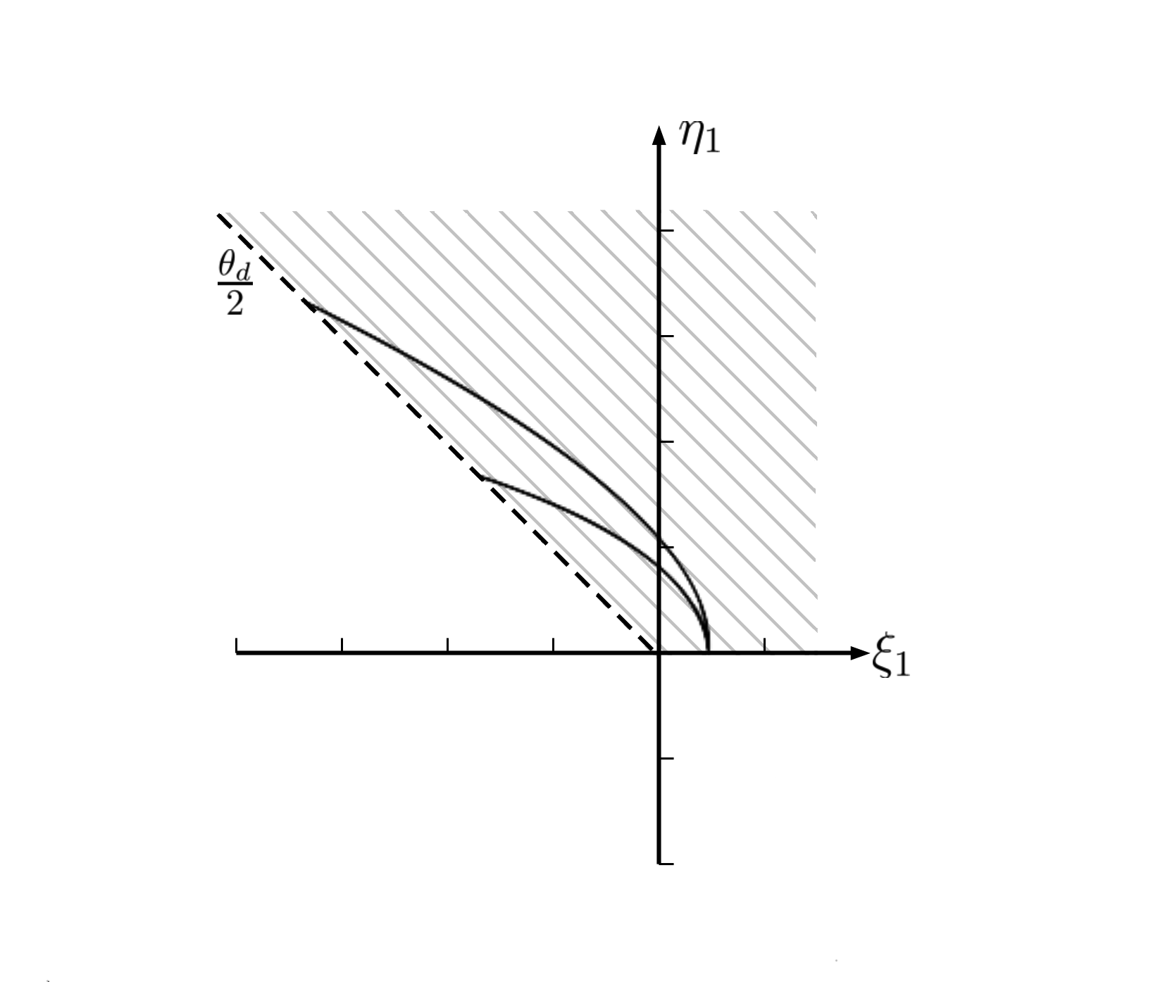
We then seek to add valid constraints on the last pair of lifted variables $(\xi_{\nu},\eta_{\nu})$. By the invariance of 2-norm of $\mathbf{Fold}$ and $\Rot$ it is easy to see that (8) and (9) imply

If $(x,y)\in\mathcal{S}_{[\ell,u]}$, by observation (3) this quantity should equal $\left(\frac{y+1}{2}\right)^{2}$. Together with the angular restriction of $(\xi_{\nu},\eta_{\nu})$, for any fixed $y$, $(\xi_{\nu},\eta_{\nu})$ must fall on the arc $\widetilde{AC}$ as in Figure 2(d), hence lies in the convex triangular region $\Delta ABC$, where

constructed by two tangent lines and one secant line. This restriction can be described by three valid inequalities of $(\xi_{\nu},\eta_{\nu})$ and $y$:

Let $B_{[\ell,u]}\subseteq\mathbb{R}^{2}$ be a (compact) superset of $\mathcal{S}_{[\ell,u]}$ constructed by simple bounds and the RLT inequalities (1),

We define two relaxation sets of $\mathcal{S}_{[\ell,u]}$ as follows:

Note that the definitions of $D_{\nu}(\ell,u)$ and $D^{+}_{\nu}(\ell,u)$ involve the nonsmooth folding operations, hence are not immediately admissible to optimization solvers. We will leave their integer formulations for the next section, while providing a formal, algebraic proof of the validity of relaxation and their approximation accuracy in the following theorem. As $\nu$ increases, both $D_{\nu}(\ell,u)$ and $D^{+}_{\nu}(\ell,u)$ converge to $\mathcal{S}_{[\ell,u]}$ very rapidly.

By replacing each $\mathcal{S}_{[\ell_{j},u_{j}]}$ ($\forall j$) with $D_{\nu}(\ell_{j},u_{j})$ we obtain relaxations for (MIQCP), whose optimal value is a valid lower bound to that of (MIQCP). With simple algebra, this relaxation can be written as:

where $f^{(i)},i=0,...,m$ are the quadratic functions in (MIQCP). By Theorem 1, for each $i=1,...,m$, the expression $\sum_{j=1}^{n}\delta_{j}^{(i)}\left(y_{j}-x_{j}^{2}\right)$ can be bounded by

Therefore if we let $(x(\nu),y(\nu),\zeta(\nu))$ to denote a global optimal solution to (14), then $(x(\nu),\zeta(\nu))$ is an almost-feasible solution to (MIQCP) with violation of the $i$-th constraint at most (15). Take $\nu\mapsto 0$ and assume $(x^{*},\zeta^{*})$ is a limit point of $(x(\nu),\zeta(\nu))$. Then by Theorem 1 and the continuity of $f^{i}\ (i=0,...,m)$, it is straightforward to see that $(x^{*},\zeta^{*})$ is a global optimal solution to (MIQCP). Analogous results can be established for the relaxation with $D^{+}(\ell_{j},u_{j})$ ($j=1,...,n$).

In the next section we will show $D_{\nu}(\bullet,\bullet)$ and $D^{+}_{\nu}(\bullet,\bullet)$ admit MILP and convex MIQCP formulations, respectively. Therefore related relaxations are computable by global solvers for convex MIQCP.

As the definitions of $D_{\nu}(\ell,u)$ and $D^{+}_{\nu}(\ell,u)$ use nonsmooth folding operations, they are not immediately admissible to most optimization solvers. The problematic constraints are the equalities in (8) and (9) involving the absolute value functions:

Note that the graph of a absolute value function in a bounded interval is simply the union of two line segments. By disjunctive programming we can model such constraints with additional binary variables [3]. Consider the following set with finite $L$ and $R$,

If $L\geq 0$ or $R\leq 0$, this set reduces to a simple convex set. So we assume $L<0$ and $R>0$. An integer formulation is:

It is easy to verify that if $(\eta,\omega)\in\mathcal{J}(L,R)$ and $z=1$, then $\omega\in[0,R]$ and $\eta=\omega$, otherwise if $z=0$ then $\omega\in[L,0]$ and $\eta=-\omega$. Therefore to derive integer formulations for $D_{\nu}(\ell,u)$ and $D^{+}_{\nu}(\ell,u)$ it suffices to derive finite bounds for the quantities inside the absolute value functions in (16). The following proposition and the subsequent remark provide the desired bounds.

References

- 1 Kurt M. Anstreicher. On convex relaxations for quadratically constrained quadratic programming. Mathematical Programming (Series B), 2012.
- 2 Kurt M. Anstreicher and Samuel Burer. Computable representations for convex hulls of low-dimensional quadratic forms. Mathematical Programming, 124(1-2):33–43, 2010.
- 3 Egon Balas. Disjunctive programming: properties of the convex hull of feasible points. Discrete Appl. Math., 89(1-3):3–44, 1998.
- 4 Xiaowei Bao, Nikolaos V. Sahinidis, and Mohit Tawarmalani. Multiterm polyhedral relaxations for nonconvex, quadratically constrained quadratic programs. Optimization Methods and Software, 24(4-5):485–504, 2009.
- 5 Pietro Belotti. COUENNE: a user’s manual. Technical report, Department of Mathematical Sciences, Clemson University, 2012.
- 6 Pietro Belotti, Jon Lee, Leo Liberti, François Margot, and Andreas Wächter. Branching and bounds tightening techniques for non-convex MINLP. Optim. Methods and Software, 24(4-5):597–634, 2009.
- 7 Aharon Ben-Tal and Arkadi Nemirovski. On polyhedral approximations of the second-order cone. Math. Oper. Res., 26(2):193–205, 2001.
- 8 Steven J. Benson and Yinyu Ye. DSDP5 user guide — software for semidefinite programming. Technical Report ANL/MCS-TM-277, Mathematics and Computer Science Division, Argonne National Laboratory, Argonne, IL, September 2005. http://www.mcs.anl.gov/~benson/dsdp.
- 9 Steven J. Benson, Yinyu Ye, and Xiong Zhang. Solving Large-Scale Sparse Semidefinite Programs for Combinatorial Optimization. SIAM Journal on Optimization, 10(2):443–461, 2000.
- 10 Benson, Hande Y., and Umit Saĝlam. Mixed-integer second-order cone programming: A survey. In Theory Driven by Influential Applications, pages 13–36. INFORMS, 2013.
- 11 Timo Berthold, Stefan Heinz, and Stefan Vigerske. Extending a CIP Framework to Solve MIQCPs. In Jon Lee and Sven Leyffer, editors, Mixed Integer Nonlinear Programming, pages 427–444, New York, NY, 2012. Springer New York.
- 12 S. Burer. On the copositive representation of binary and continuous nonconvex quadratic programs. Mathematical Programming, 120:479–495, 2009.
- 13 Samuel Burer and Hongbo Dong. Representing quadratically constrained quadratic programs as generalized copositive programs. Operations Research Letters, 40(3):203–206, May 2012.
- 14 Samuel A. Burer and Jieqiu Chen. Globally solving nonconvex quadratic programming problems via completely positive programming. Mathematical Programming Computation, 4:33–52, 2012.
- 15 M. Bynum, A. Castillo, J. Watson, and C. D. Laird. Tightening McCormick Relaxations Toward Global Solution of the ACOPF Problem. IEEE Transactions on Power Systems, 2018.
- 16 Mary B. Cain, Richard P. O’neill, and Anya Castillo. History of optimal power flow and formulations. Technical report, Cain, Mary B. and Richard P. O’neill and Anya Castillo, 2012.
- 17 Hongbo Dong. Relaxing nonconvex quadratic functions by multiple adaptive diagonal perturbations. SIAM Journal on Optimization, 26(3):1962–1985, 2016.
- 18 M. Duran and I. Grossmann. An outer-approximation algorithm for a class of mixedinteger nonlinear programs. Mathematical Programming, 36(3):307–339, 1986.
- 19 Yong Fu, Mohammad Shahidehpour, and Zuyi Li. Security-Constrained Unit Commitment With AC Constraints. IEEE Transactions on Power Systems, 20(3):1538–1550, 2005.
- 20 Fabio Furini, Emiliano Traversi, Pietro Belotti, Antonio Frangioni, Ambros Gleixner, Nick Gould, Leo Liberti, Andrea Lodi, Ruth Misener, Hans Mittelmann, Nikolaos Sahinidis, Stefan Vigerske, and Angelika Wiegele. Qplib: A library of quadratic programming instances. Mathematical Programming Computation, 2018.
- 21 Bissan Ghaddar, Jakub Marecek, and Martin Mevissen. Optimal power flow as a polynomial optimization problem. IEEE transaction on Power Systems, 31(1):539–546, Jan 2016.
- 22 Ambros Gleixner, Michael Bastubbe, Leon Eifler, Tristan Gally, Gerald Gamrath, Robert Lion Gottwald, Gregor Hendel, Christopher Hojny, Thorsten Koch, Marco E. Lübbecke, Stephen J. Maher, Matthias Miltenberger, Benjamin Müller, Marc E. Pfetsch, Christian Puchert, Daniel Rehfeldt, Franziska Schlösser, Christoph Schubert, Felipe Serrano, Yuji Shinano, Jan Merlin Viernickel, Matthias Walter, Fabian Wegscheider, Jonas T. Witt, and Jakob Witzig. The SCIP Optimization Suite 6.0. ZIB-Report 18-26, Zuse Institute Berlin, July 2018.
- 23 M.X. Goemans and D.P. Williamson. Improved approximation algorithms for maximum cut and satisfiability problems using semidefinite programming. Journal of ACM, 42:1115–1145, 1995.
- 24 Gurobi Optimization, Inc. Gurobi Optimizer Reference Manual, 2018.
- 25 Joey Huchette and Juan Pablo Vielma. A combinatorial approach for small and strong formulations of disjunctive constraints. To appear in Mathematics of Operations Research, 2018.
- 26 IBM Corporation. IBM ILOG CPLEX Optimization Studio 12.7, User Manual, 2017.
- 27 Burak Kocuk, Santanu Dey, and X Sun. Strong SOCP relaxations for the optimal power flow problem. Oper Res, 2016.
- 28 Burak Kocuk, Santanu S. Dey, and X. Andy Sun. Matrix minor reformulation and socp-based spatial branch-and-cut method for the ac optimal power flow problem. Mathematical Programming Computation, 10(4):557–596, Dec 2018.
- 29 Burak Kocuk, Santanu S. Dey, and Xu Andy Sun. New formulation and strong MISOCP relaxations for AC optimal transmission switching problem. IEEE Transactions on Power Systems, 32(6):4161–4170, 2017.
- 30 Nathan Krislock, Jérôme Malick, and Frédéric Roupin. Improved semidefinite branch-and-bound algorithm for k-cluster. Revision submitted to Computers and Operations Research, https://hal.archives-ouvertes.fr/hal-00717212, Nov. 2013.
- 31 Nathan Krislock, Jérôme Malick, and Frédéric Roupin. Improved semidefinite bounding procedure for solving Max-Cut problems to optimality. Mathematical Programming, 143(1-2):61–86, 2014.
- 32 Sven Leyffer. Deterministic methods for mixed integer nonlinear programming. Ph.D. thesis, University of Dundee, 1993.
- 33 Youdong Lin and Linus Schrage. The global solver in the LINDO API. Optimization Methods & Software, 24(4–5):657–668, Aug. 2009.
- 34 Miles Lubin and Iain Dunning. Computing in operations research using julia. INFORMS Journal on Computing, 27(2):238–248, 2015.
- 35 R. Misener and C. A. Floudas. ANTIGONE: Algorithms for coNTinuous / Integer Global Optimization of Nonlinear Equations. Journal of Global Optimization, 2014.
- 36 Ruth Misener and Christodoulos Floudas. Global optimization of mixed-integer quadratically-constrained quadratic programs (MIQCQP) through piecewise-linear and edge-concave relaxations. Math Program, 136(1):155–182, 2012.
- 37 Javier Peña, Juan C. Vera, and Luis F Zuluaga. Completely positive reformulations for polynomial optimization. Mathematical Programming, 151(2):405–431, Jul. 2015.
- 38 S. Poljak, F. Rendl, and H. Wolkowicz. A recipe for semidefinite relaxation for 0-1 quadratic programming. Journal of Global Optimization, 7:51–73, 1995.
- 39 Franz Rendl, Giovanni Rinaldi, and Angelika Wiegele. Solving Max-Cut to optimality by intersecting semidefinite and polyhedral relaxations. Math. Program., Ser. A, 121:307–335, 2010.
- 40 N. V. Sahinidis. BARON 17.8.9: Global Optimization of Mixed-Integer Nonlinear Programs. User’s manual, 2017.
- 41 Anureet Saxena, Pierre Bonami, and Jon Lee. Convex relaxations of mixed integer quadratically constrained programs: Extended formulations. Research report, IBM, Yorktown Heights, NY, 2008. To appear in Mathematical Programming.
- 42 Anureet Saxena, Pierre Bonami, and Jon Lee. Convex relaxations of mixed integer quadratically constrained programs: Projected formulations. Mathematical Programming, Series A, 130(2):359–413, 2011.
- 43 N.Z. Shor. Quadratic optimization problems. Soviet Journal of Computer and Systems Science, 25:1–11, 1987. Originally published in Tekhnicheskaya Kibernetika, 1:128–139, 1987.
- 44 The Optimization Firm. NLP and MINLP Test Problems.
- 45 J. P. Vielma. Mixed integer linear programming formulation techniques. SIAM Review, 57:3–57, 2015.
- 46 J. P. Vielma and G. Nemhauser. Modeling disjunctive constraints with a logarithmic number of binary variables and constraints. Mathematical Programming, 128:49–72, 2011.
- 47 Juan Pablo Vielma, Shabbir Ahmed, and George L. Nemhauser. A lifted linear programming branch-and-bound algorithm for mixed-integer conic quadratic programs. INFORMS J. Comput., 20(3):438–450, 2008.
- 48 Stefan Vigerske and Ambros Gleixner. Scip: global optimization of mixed-integer nonlinear programs in a branch-and-cut framework. Optimization Methods and Software, 33(3):563–593, 2018.
- 49 A. Vinel and P. Krokhmal. Polyhedral approximations in -order cone programming. Optim. Methods and Software, 160:439–456, 2014.
- [1] Kurt M. Anstreicher. On convex relaxations for quadratically constrained quadratic programming. Mathematical Programming (Series B), 2012.
- [2] Kurt M. Anstreicher and Samuel Burer. Computable representations for convex hulls of low-dimensional quadratic forms. Mathematical Programming, 124(1-2):33–43, 2010.
- [3] Egon Balas. Disjunctive programming: properties of the convex hull of feasible points. Discrete Appl. Math., 89(1-3):3–44, 1998.
- [4] Xiaowei Bao, Nikolaos V. Sahinidis, and Mohit Tawarmalani. Multiterm polyhedral relaxations for nonconvex, quadratically constrained quadratic programs. Optimization Methods and Software, 24(4-5):485–504, 2009.
- [5] Pietro Belotti. COUENNE: a user’s manual. Technical report, Department of Mathematical Sciences, Clemson University, 2012.
- [6] Pietro Belotti, Jon Lee, Leo Liberti, François Margot, and Andreas Wächter. Branching and bounds tightening techniques for non-convex MINLP. Optim. Methods and Software, 24(4-5):597–634, 2009.
- [7] Aharon Ben-Tal and Arkadi Nemirovski. On polyhedral approximations of the second-order cone. Math. Oper. Res., 26(2):193–205, 2001.
- [8] Steven J. Benson and Yinyu Ye. DSDP5 user guide — software for semidefinite programming. Technical Report ANL/MCS-TM-277, Mathematics and Computer Science Division, Argonne National Laboratory, Argonne, IL, September 2005. http://www.mcs.anl.gov/~benson/dsdp.
- [9] Steven J. Benson, Yinyu Ye, and Xiong Zhang. Solving Large-Scale Sparse Semidefinite Programs for Combinatorial Optimization. SIAM Journal on Optimization, 10(2):443–461, 2000.
- [10] Benson, Hande Y., and Umit Saĝlam. Mixed-integer second-order cone programming: A survey. In Theory Driven by Influential Applications, pages 13–36. INFORMS, 2013.
- [11] Timo Berthold, Stefan Heinz, and Stefan Vigerske. Extending a CIP Framework to Solve MIQCPs. In Jon Lee and Sven Leyffer, editors, Mixed Integer Nonlinear Programming, pages 427–444, New York, NY, 2012. Springer New York.
- [12] S. Burer. On the copositive representation of binary and continuous nonconvex quadratic programs. Mathematical Programming, 120:479–495, 2009.
- [13] Samuel Burer and Hongbo Dong. Representing quadratically constrained quadratic programs as generalized copositive programs. Operations Research Letters, 40(3):203–206, May 2012.
- [14] Samuel A. Burer and Jieqiu Chen. Globally solving nonconvex quadratic programming problems via completely positive programming. Mathematical Programming Computation, 4:33–52, 2012.
- [15] M. Bynum, A. Castillo, J. Watson, and C. D. Laird. Tightening McCormick Relaxations Toward Global Solution of the ACOPF Problem. IEEE Transactions on Power Systems, 2018.
- [16] Mary B. Cain, Richard P. O’neill, and Anya Castillo. History of optimal power flow and formulations. Technical report, Cain, Mary B. and Richard P. O’neill and Anya Castillo, 2012.
- [17] Hongbo Dong. Relaxing nonconvex quadratic functions by multiple adaptive diagonal perturbations. SIAM Journal on Optimization, 26(3):1962–1985, 2016.
- [18] M. Duran and I. Grossmann. An outer-approximation algorithm for a class of mixedinteger nonlinear programs. Mathematical Programming, 36(3):307–339, 1986.
- [19] Yong Fu, Mohammad Shahidehpour, and Zuyi Li. Security-Constrained Unit Commitment With AC Constraints. IEEE Transactions on Power Systems, 20(3):1538–1550, 2005.
- [20] Fabio Furini, Emiliano Traversi, Pietro Belotti, Antonio Frangioni, Ambros Gleixner, Nick Gould, Leo Liberti, Andrea Lodi, Ruth Misener, Hans Mittelmann, Nikolaos Sahinidis, Stefan Vigerske, and Angelika Wiegele. Qplib: A library of quadratic programming instances. Mathematical Programming Computation, 2018.
- [21] Bissan Ghaddar, Jakub Marecek, and Martin Mevissen. Optimal power flow as a polynomial optimization problem. IEEE transaction on Power Systems, 31(1):539–546, Jan 2016.
- [22] Ambros Gleixner, Michael Bastubbe, Leon Eifler, Tristan Gally, Gerald Gamrath, Robert Lion Gottwald, Gregor Hendel, Christopher Hojny, Thorsten Koch, Marco E. Lübbecke, Stephen J. Maher, Matthias Miltenberger, Benjamin Müller, Marc E. Pfetsch, Christian Puchert, Daniel Rehfeldt, Franziska Schlösser, Christoph Schubert, Felipe Serrano, Yuji Shinano, Jan Merlin Viernickel, Matthias Walter, Fabian Wegscheider, Jonas T. Witt, and Jakob Witzig. The SCIP Optimization Suite 6.0. ZIB-Report 18-26, Zuse Institute Berlin, July 2018.
- [23] M.X. Goemans and D.P. Williamson. Improved approximation algorithms for maximum cut and satisfiability problems using semidefinite programming. Journal of ACM, 42:1115–1145, 1995.
- [24] Gurobi Optimization, Inc. Gurobi Optimizer Reference Manual, 2018.
- [25] Joey Huchette and Juan Pablo Vielma. A combinatorial approach for small and strong formulations of disjunctive constraints. To appear in Mathematics of Operations Research, 2018.
- [26] IBM Corporation. IBM ILOG CPLEX Optimization Studio 12.7, User Manual, 2017.
- [27] Burak Kocuk, Santanu Dey, and X Sun. Strong SOCP relaxations for the optimal power flow problem. Oper Res, 2016.
- [28] Burak Kocuk, Santanu S. Dey, and X. Andy Sun. Matrix minor reformulation and socp-based spatial branch-and-cut method for the ac optimal power flow problem. Mathematical Programming Computation, 10(4):557–596, Dec 2018.
- [29] Burak Kocuk, Santanu S. Dey, and Xu Andy Sun. New formulation and strong MISOCP relaxations for AC optimal transmission switching problem. IEEE Transactions on Power Systems, 32(6):4161–4170, 2017.
- [30] Nathan Krislock, Jérôme Malick, and Frédéric Roupin. Improved semidefinite branch-and-bound algorithm for k-cluster. Revision submitted to Computers and Operations Research, https://hal.archives-ouvertes.fr/hal-00717212, Nov. 2013.
- [31] Nathan Krislock, Jérôme Malick, and Frédéric Roupin. Improved semidefinite bounding procedure for solving Max-Cut problems to optimality. Mathematical Programming, 143(1-2):61–86, 2014.
- [32] Sven Leyffer. Deterministic methods for mixed integer nonlinear programming. Ph.D. thesis, University of Dundee, 1993.
- [33] Youdong Lin and Linus Schrage. The global solver in the LINDO API. Optimization Methods & Software, 24(4–5):657–668, Aug. 2009.
- [34] Miles Lubin and Iain Dunning. Computing in operations research using julia. INFORMS Journal on Computing, 27(2):238–248, 2015.
- [35] R. Misener and C. A. Floudas. ANTIGONE: Algorithms for coNTinuous / Integer Global Optimization of Nonlinear Equations. Journal of Global Optimization, 2014.
- [36] Ruth Misener and Christodoulos Floudas. Global optimization of mixed-integer quadratically-constrained quadratic programs (MIQCQP) through piecewise-linear and edge-concave relaxations. Math Program, 136(1):155–182, 2012.
- [37] Javier Peña, Juan C. Vera, and Luis F Zuluaga. Completely positive reformulations for polynomial optimization. Mathematical Programming, 151(2):405–431, Jul. 2015.
- [38] S. Poljak, F. Rendl, and H. Wolkowicz. A recipe for semidefinite relaxation for 0-1 quadratic programming. Journal of Global Optimization, 7:51–73, 1995.
- [39] Franz Rendl, Giovanni Rinaldi, and Angelika Wiegele. Solving Max-Cut to optimality by intersecting semidefinite and polyhedral relaxations. Math. Program., Ser. A, 121:307–335, 2010.
- [40] N. V. Sahinidis. BARON 17.8.9: Global Optimization of Mixed-Integer Nonlinear Programs. User’s manual, 2017.
- [41] Anureet Saxena, Pierre Bonami, and Jon Lee. Convex relaxations of mixed integer quadratically constrained programs: Extended formulations. Research report, IBM, Yorktown Heights, NY, 2008. To appear in Mathematical Programming.
- [42] Anureet Saxena, Pierre Bonami, and Jon Lee. Convex relaxations of mixed integer quadratically constrained programs: Projected formulations. Mathematical Programming, Series A, 130(2):359–413, 2011.
- [43] N.Z. Shor. Quadratic optimization problems. Soviet Journal of Computer and Systems Science, 25:1–11, 1987. Originally published in Tekhnicheskaya Kibernetika, 1:128–139, 1987.
- [44] The Optimization Firm. NLP and MINLP Test Problems.
- [45] J. P. Vielma. Mixed integer linear programming formulation techniques. SIAM Review, 57:3–57, 2015.
- [46] J. P. Vielma and G. Nemhauser. Modeling disjunctive constraints with a logarithmic number of binary variables and constraints. Mathematical Programming, 128:49–72, 2011.
- [47] Juan Pablo Vielma, Shabbir Ahmed, and George L. Nemhauser. A lifted linear programming branch-and-bound algorithm for mixed-integer conic quadratic programs. INFORMS J. Comput., 20(3):438–450, 2008.
- [48] Stefan Vigerske and Ambros Gleixner. Scip: global optimization of mixed-integer nonlinear programs in a branch-and-cut framework. Optimization Methods and Software, 33(3):563–593, 2018.
- [49] A. Vinel and P. Krokhmal. Polyhedral approximations in -order cone programming. Optim. Methods and Software, 160:439–456, 2014.