SLAC–PUB–17356 November, 2018
Fermion Pair Production in Gauge-Higgs Unification Models
Jongmin Yoon and Michael E. Peskin11 1 Work supported by the US Department of Energy, contract DE–AC02–76SF00515.
SLAC, Stanford University, Menlo Park, California 94025 USA
ABSTRACT
We compute fermion pair production cross sections in annihilation in models of electroweak symmetry breaking in warped 5-dimensional space. Our analysis is based on a framework with no elementary scalars, only gauge bosons and fermions in the bulk. We apply a novel Green’s function method to obtain an analytic understanding of the new physics effects across the parameter space. We present results for and . The predicted effects will be visible in precision measurements. Different models of quark mass generation can be distinguished by these measurements already at 250 GeV in the center of mass.
Submitted to Physical Review D
1 Introduction
The Standard Model (SM) gives an excellent description of physics at the energies that we now explore at accelerators. But still it is a compelling idea that the SM is incomplete. If there is an explanation for the electroweak symmetry breaking of the SM and the magnitudes of the quark and lepton masses, this requires a generalization of the SM with new fundamental interactions associated with the Higgs field.
Many extensions of the SM have been explored theoretically. However, it is our opinion that there is still much to learn about models in which the Higgs field is composite [1, 2]. In a series of papers [3, 4], we have attempted to gain new insight into this class of models by considering these models in a Randall-Sundrum framework [5] in which the SM is extended to 5-dimensional anti-de Sitter space. The gauge group of the SM can be enlarged so that the Higgs doublet can appear as the 5th components of gauge fields [6, 7]. In this context, it is possible to compute the Higgs potential and find a dynamical origin for electroweak symmetry breaking [8].
In [4] we examined in some detail a particular model based on gauge symmetry in the 5-dimensional bulk. This follows a path defined about ten years ago by Agashe, Contino, and Pomarol [9]. By making use of some new model-building strategies, we were able to find a class of models with an adjustible hierarchy between the electroweak scale and the mass scale of the intrinsically 5D dynamics. Specifically, this “little hierarchy” is controlled by a mixing angle parametrized by . The little hierarchy must be large to avoid constraints from precision electroweak measurements. Then is small and can be used as an expansion parameter. The predictions of the model can be expressed as corrections to SM formulae of order and higher, and this presentation gives useful insight into their structure.
In this paper, we continue this study by describing the implications of measurements of quark and lepton pair production. For definiteness, we consider in detail the reaction , where the electron is assumed to be structureless, that is, confined to the extreme UV region of the 5D Randall-Sundrum space. This physics has been explored previously by Funatsu, Hatanaka, Hosotani, and Orikasa in [10]. We show here that there is not a unique prediction for the modification of the cross section, but, rather, a discrete set of predictions depending on the scheme for producing the mass of the quark.
In [4], we generated the mass of the top quark through dynamical symmetry breaking. In that paper, we left open the question of how the lighter quarks and leptons receive their masses. These must arise by feed-down from the top quark mass. The flavor mixing should occur at high energies, above the scale at which the top quark mass is generated. According to the dictionary linking the 5D and 4D descriptions of the theory, this mixing involving the light fermions should be represented by a boundary condition on the UV boundary of the Randall-Sundrum space. Here, we will describe several distinct scenarios for this flavor mixing and show that these are reflected in different predictions for observable cross sections. Typically, the effects become large enough to be observed at 500 GeV in the center of mass, but in some cases we find observable deviations from the SM at 250 GeV.
Our analysis has a straightforward extension to . Corrections to the cross section in RS models have been studied in numerous references, reviewed in [11], and additional model predictions been presented more recently in [12]. We believe that our analytic approach to the parameter space of RS models contains new insight into the size and nature of the expected effects.
The outline of this paper is as follows: In Section 2, we review well-known results on for massless fermions with unbroken gauge symmetry (Randall-Sundrum QED) [13], and show how these follow from the formalism of [4]. In Section 3, we review the features of the 5D RS model that are essential for our discussion here. In Section 4, we present the structure of the electroweak boson propagators in this model. In Section 5, we describe schemes for generating the mass of the quark in our model and work out the implications of each for the helicity-dependent cross sections in . Precision measurements of at an collider, even at 250 GeV, can distinguish these models. In Section 6, we generalize this analysis to the computation of the helicity-dependent cross sections for and present our numerical predictions. The resulting effects are large enough to be readily discovered in precision collider experiments. Section 7 gives our conclusions.
2 Randall-Sundrum QED
In this section we review results on the process mediated by a bulk gauge field in the Randall-Sundrum space. We begin our discussion with the basic formalism for RS geometry and 5D bulk fields. The notation follows that of [3] and [4].
2.1 Overview
We consider a model of gauge and fermion fields living in the interior of a slice of 5-dimensional anti-de Sitter space
| (1) |
with nontrivial boundary conditions at and , with . Then gives the position of the “UV brane” and gives the position of the “IR brane”. The perhaps more physical metric
| (2) |
is related by . We take the size of the interval in to be . Then
| (3) |
The scales and set the ultraviolet and infrared boundaries of the dynamics described by the 5D fields.
The bulk action of gauge fields and fermions in RS is
| (4) |
We will notate gauge fields as , where , with lower case . Fermion fields are 4-component Dirac fields. Here, we will typically break these up into 2-component spinors with negative and positive 4D chirality: . We will parametrize the 5D Dirac mass using the dimensionless parameter . In principle, this parameter is different for each gauge multiplet of fermion fields. In our formalism, the Higgs field is a background gauge field, so we will quantize in the Feynman-Randall-Schwartz background field gauge [14].
For concreteness, we will be interested in values of of order 1 TeV and values of of order 100 TeV. Thus, we imagine that is at a flavor dynamics scale rather than at the Planck scale. Still, it will be accurate to ignore terms of order , and we will do so throughout our calculations. We will not ignore terms of order or, more generally, terms of order .
The physics beyond the UV cutoff scale can affect the dynamics of the 5D theory. To model this, we apply nontrivial boundary conditions on the UV brane. First, we will allow mixing of fermions that belong to different gauge multiplets in the bulk but have the same quantum numbers under the SM subgroup of the bulk gauge group. Second, we include localized kinetic terms on the UV brane for the gauge fields and fermions:
| (5) |
where , are constant parameters. A similiar term for is also allowed but will not be used here. In either case, for the fermions, the boundary term has a substantial effect only for a field that has a UV-localized zero-mode. The formalism of the boundary kinetic terms is discussed in detail in [4].
We will work in Fourier space for the four extended dimensions and in coordinate space for the 5th, warped, dimension. The solutions of field equations in the RS geometry with fixed Minkowski momenta are then given in terms of Bessel functions in the form [15, 16, 17]
| (6) |
It is useful to define combinations of the Bessel functions so that the solutions (6), as a function of , have definite boundary conditions at a point . Thus we set
| (7) |
where . For solutions to the Dirac equation, the orders of the Bessel functions depend on the parameter according to
| (8) |
For gauge fields, the same combinations of Bessel functions apply with , with giving the solutions for and giving the solutions for . For gauge fields , , give solutions with Neumann and Dirichlet boundary conditions, respectively, at . For fermions , , give solutions with and , respectively, at . In the rest of paper, we will denote these boundary conditions by or . For example, represents Neumann or boundary condition on the UV brane and Dirichlet or boundary condition on the IR brane. Further discussion of our formalism and additional properties of the Green’s functions are given in the appendices of [4].
In general, in this paper, when a function appears without arguments, it is
| (9) |
For fields with a boundary kinetic term with coefficient , we will find it convenient to define
| (10) |
We define further
| (11) |
For , the case of a bulk gauge field, and gives the relation between the 5D coupling constant and the (dimensionless) 4D coupling constant,
| (12) |
2.2 Chiral fermion wavefunctions
Massive fermions in 5D have nonzero components for both and . However, with appropriate boundary conditions, 5D fermion fields can have zero modes that can be interpreted as chiral quarks and leptons [17, 18].
A left-handed fermion zero mode has the form
| (13) |
where is the usual 2-component massless spinor. Solving the RS Dirac equation, we find that the zero mode has the form
| (14) |
We have normalized the zero mode wavefunction so that
| (15) | |||||
Notice that, according to (14) or (15), a finite contribution to the normalization integral is contained in a singular piece of the wavefunction at . Away from this point, the fermion wavefunction is smooth. In the following sections, we will need to compute expectation values in the 5D fermion wavefunctions. It is convenient to use the formula
| (16) |
This avoids explicit consideration of the singularity at . Some further discussion of this point is given in Appendix A.
A right-handed fermion zero mode has the form
| (17) |
where is the usual 2-component right-handed massless spinor. The function is obtained from by sending and, for our choice of boundary conditions, setting .
For , is localized near the UV brane. That is, we can consider the wave-function of the UV-localized zero mode as well approximated by delta function at :
| (18) |
For a left-handed zero mode, the boundary kinetic term can make a substantial effect only if . In this case, shifts the wavefunction further towards the UV boundary. For , the right-handed zero mode is localized near the IR brane and therefore its boundary term would have negligible effect. It is therefore justified to ignore possible boundary term for IR-localized zero-modes.
Eventually, the zero-mode fermions will obtain mass by mixing of a left-handed zero mode with a right-handed zero mode. We will discuss schemes for mass generation for the quark in Sections 5. However, if we generate masses that are small compared to , it will always be a good approximation to neglect the direct effects of the masses and mixings in the computation of cross sections. Since the components of gauge bosons have matrix elements only between and components of fermion fields, we will then also neglect exchange.
2.3 in RS
Using the Feynman-Randall-Schwartz gauge fixing with , we can compute the Green’s functions for gauge fields
| (19) |
The details of the Green’s function computation can be found in the appedix of [4]. For a non-Abelian bulk gauge group, will be a matrix in the group indices.
Combining this with the description of light fermions given in the previous section, we can write the scattering amplitude for the -channel pair production involving fermions of definite helicity as
| (20) |
Here the subscripts , denote the chiralities of the initial and final fermions and the -channel amplitude is given by
| (21) |
where are the zero mode wavefunctions of the initial and final fermions and and are the quantum numbers of and under the symmetry. (For a non-Abelian group, will be generalized to a vector of gauge charges.) We use the notation that includes the 5D gauge coupling .
The spinor and Lorentz structure of (20) is the same as that in a 4D calculation of the same cross section. Therefore, the effect of the RS dynamics on each individual helicity amplitude is given simply by replacing the -channel vector boson propagator by the quantity in (21). In the simplest case of QED, this multiplies the scattering amplitude by the factor
| (22) |
We can view this expression either as a form factor for the photon or, for , as an unmodified photon propagator plus a contact interaction representing the Kaluza-Klein (KK) states.
In this paper, we will focus on the reactions , where the left- and right-handed electrons are assumed to be approximately structureless, that is, associated with zero modes localized close to the UV brane. Then simplifies to
| (23) |
In the rest of this paper, including examples in which is a matrix, we abbreviate
| (24) |
so the takes the simple form
| (25) |
If the fermion has a UV boundary kinetic term, (23) and (24) should be modified accordingly to include its effect as in (15) and (16).
If the fermion is also extremely localized in the UV, reduces to its form in the SM up to small corrections. However, we can obtain nontrivial effects if the zero mode extends into the infrared, or, in the language of RS phenomenology, the is partially composite.
2.4 Pair production in RS with bulk symmetry
Using this formalism, we can compute the modification of the reactions under a bulk gauge symmetry. For definiteness, we consider the case in which the charges of the zero mode fermions are equal to 1, so that . Then the modification factor (22) is the same for all four cases of fermion helicity. We will consider the field to have a UV boundary kinetic term with coefficient . We will work out the implications of this model for the various choices of and boundary conditions of the gauge field.
First, consider the boundary condition. The gauge field includes a massless photon and its KK resonances. The gauge boson propagator in this case is computed in Appendix C of [4] and found to take the form
| (26) |
where () is the smaller (larger) of and . The form is rather intuitive; the Green’s function satisfies the correct boundary conditions at both the UV and the IR boundaries. The prescription (10) modifies the UV boundary condition on the Green’s function to account for the delta function kinetic term on the boundary. For , we set and find
| (27) |
where we have used (11). The quantity in the expectation value goes to 1 for .
We can get further insight by expanding the expression (27) for low energy reactions. Assuming that the center of mass energy is smaller than the scale of the IR brane, we expand the Bessel functions in around . In this expansion, we will ignore corrections of order . Including the first corrections in , we obtain an approximate formula
| (28) |
where we have introduced the 4D gauge coupling as in (12). In this low-energy effective form, the first correction to the massless photon exchange appears as a dimension-6 contact interaction. The contact interaction describes the effect of massive KK boson exchanges. The strength of the contact interaction is given by
| (29) |
Note that the effect of the gauge boundary term always appears in the form of . If the final state fermions are UV-localized, the latter two terms in (29) are of order and is negative. On the other hand, if the final state fermion is confined in the IR brane, the sum of the two terms is 1 and is maximized. From this, we obtain an upper bound .
It is well known that, for zero boundary kinetic terms, the Kaluza-Klein corrections to scattering in RS vanish if . At this value, the fermion wavefunctions in the coordinate system (2) are constant in and so the fermion currents are orthogonal to the KK gauge boson wavefunctions [15, 16]. In the presence of the boundary terms, there are also significant cancellations. In the expansion, we find, using (16),
| (30) |
where . If we further have , we find that . Actually, it is not difficult to show that,
| (31) |
as an exact result.
Next we consider the other boundary conditions, where the symmetry is broken in either UV or IR boundary. Those 5D gauge fields do not include a massless mode. For a boundary condition, we find
| (32) |
Then
| (33) | |||||
We have only the contact interaction. Notice that the UV boundary kinetic term has no effect at low energy if there is no massless gauge field.
For a boundary condition, we have
| (34) |
Then, when the UV-localized electron is in the UV, we have , because vanishes as . The result is easy to understand geometrically: A gauge field with UV boundary condition does not couple to a UV-localized electron. Similarly, for the boundary condition, we have
| (35) |
and again .
3 Model of Gauge-Higgs Unification
In this section, we review the elements of the model that are essential for our study of . Further details of the model can be found in [4].
3.1 Group structure and boundary conditions
For a realistic model, we choose its bulk gauge symmetry to be [9]. Boundary conditions break the bulk symmetry to the SM gauge symmetry on the UV brane and to on the IR brane. This model can be viewed as a dual description of an approximately conformal dynamics between the scales and in four dimensions. In the dual 4D interpretation, the system has a global symmetry , of which subgroup is gauged to a local symmetry. The strongly interacting theory spontaneously breaks to the subgroup at the scale . The extra factor in is a custodial symmetry that protects the relation from receiving large corrections [19]. The study of the 5D model gives a calculable approach to the 4D theory.
We label the 10 generators of as , , , , with . The generators , generate the subgroup of . The first here is identified with the weak interaction gauge group. The generator of the is labelled . We assign the boundary condtions
| (36) |
for , . Let and be the 5D gauge couplings of and . Introduce an angle such that
| (37) |
We assign the combinations
| (38) |
to have the boundary conditions
| (39) |
In all, there are four 5D gauge bosons, giving four zero modes that can be associated with the four 4D gauge bosons of .
The boundary conditions on the gauge fields are the opposite of those written above for . Then the fields have zero modes that are associated with scalars in 4D. These are the Goldstone bosons resulting from the spontaneous breaking of to .
In terms of the gauge fields with definite boundary conditions, the 5D covariant derivative is
| (40) |
summed over , , . The 5D hypercharge coupling is given by . The hypercharge and electric charge are given by
| (41) |
where is the charge.
Lastly, we include UV boundary kinetic terms and for the bosons. From the point of view of duality, the values of the gauge couplings would be set at some much larger energy scale, perhaps at the scale of grand unification. These settings would appear in the RS model as boundary conditions on the UV brane. We use the boundary kinetic terms to parametrize the effect.
Explicit formulae for the representation matrices described in this section are given in Appendix B of [4].
3.2 Identification of the Higgs field
The four zero-modes transform as a doublet under . These have precisely the quantum numbers of the complex doublet of Higgs fields.
Because the Higgs fields appear as components of gauge fields, we can gauge away their vacuum expectation values in the central region of . However, in a 5D system with boundaries, we cannot gauge away these background fields completely. Instead, such a gauge transformation leaves singular fields at or . We can parametrize the gauge-invariant information of the background fields in terms of a Wilson line element from to . The Coleman-Weinberg potential of the Higgs field will depend on this variable [3].
We can align the expectation value along the direction. Then the Wilson line element becomes
| (42) |
where is the Higgs field normalization constant:
| (43) |
The Goldstone boson decay constant is analogous to the pion decay constant in QCD. The separation between and represents the ‘little hierarchy’ between the weak interaction scale and the scale of 5D physics. Since the KK excitations are not yet observed, must be small. Therefore, we can use as an expansion parameter in our study of .
3.3 Gauge choice
When we gauge away the Higgs field in the interior of the RS space, we have a choice whether to move it to the UV or the IR boundary. We will refer to the first case, in which acts on the UV boundary, as the UV gauge and to the second case as the IR gauge.
In the UV gauge, we have definite boundary conditions for the fields on the IR brane. The Green’s functions in this gauge are most simply written in terms of functions pivoted at , e.g., , which satisfy the IR boundary conditions manifestly. Since these functions are already independent of , this choice makes it easier to take the limit , which will simplify our expressions.
On the other hand, the IR gauge also gives attractive simplifications. We have seen examples of these in the discussion of precision electroweak corrections in [4]. It is a general property that boundary mixing terms for two fields with identical boundary conditions have no effect. For example, we can apply this to the vector fields and . These have the same boundary condition in the IR, and so some expressions generated by the mixing (38) disappear in the IR gauge. Similarly, as we will discuss below, the expressions for zero-mode wavefunctions are generally simpler in the IR gauge.
It would be best if we could utilize the advantages of the both gauge choices, using for gauge Green’s functions as well as having unmixed boundary conditions for the gauge field and fermion zero-modes. A convenient prescription is to compute Green’s functions in the UV gauge but then transform to the IR gauge using the relation
| (44) |
Some consequences of this formula are discussed in [4], and an explicit proof of the formula is given in Appendix D of that paper.
3.4 Parametrization of the model space
With our set-up of the model, the masses of the W and Z bosons are given, to leading order in , by [4]
| (45) |
where and similarly for . For and TeV, we need to obtain the measured value of the mass. We define basic values of the 4D gauge coupling , the SM Higgs vacuum expectation value , and the weak mixing angle by
| (46) |
With these choices, the vector boson masses and cross sections obey the tree-level SM relations. Corrections to those relations appear at the next order in . The most important of these are computed in Section 6 of [4].
The mass of the W boson is determined by , , and . We choose and as the two main parameters of our study. gives the scale of the new strong dynamics and parametrizes the ‘little hierarchy’, that is, the degree of fine tuning between the electroweak scale and the new dynamics. The boundary kinetic term allows us the freedom to fit the W boson mass for our given choice of and .
In an explicit RS model, the value of is determined by the minimization of the Coleman-Weinberg potential for the Higgs field. In [4], we studied a particular model of gauge symmetry where the top quark competes with a vector-like fermion multiplet to generate the correct Higgs potential for the observed Higgs mass. This strategy is general and can be applied to other models of gauge-Higgs unification. Even restricting to the choice of symmetry, we can have many different realistic models depending on the field content in the RS bulk.
However, when we compute the cross sections for with SM final states, the expressions that we obtain depend on these choices only through the parameters and . Our expressions will depend on the representations chosen for the SM fermions, and on the parameters of these multiplets. But, beyond this, our results will be correct in full generality for any gauge-Higgs unification model based on symmetry.
4 Pair-production of fermions in the model
Using an expansion in the small parameters and , we can obtain useful insight into the structure of the Green’s function in the model. In this section, we present a general expression for the propagator of neutral gauge fields and apply it to the process with the simplest final states, UV-localized massless fermions.
4.1 Neutral boson propagator
Using the formalism described in [4], we can compute the matrix in the IR gauge for the neutral gauge fields of the model. The full expression for is given in Appendix B. Its low-energy effective expression for the -channel boson exchange is given by
| (47) | |||||
The expression (47) is composed of the three contributions, associated respectively with the massless photon, the Z boson, and the contact interaction. The photon propagator is protected from corrections. On the Z pole, the couplings to the initial and final state fermions factorize. The couplings are expressed in terms of , and , where and are the SM coupling and the Weinberg mixing angle. An additional ‘charge’ is also defined for composite final state fermions. To order , the expressions for , , and are
| (48) |
It is instructive to note that is the only term that includes an explicit dependence on and . All other terms of are written in terms of the quantum numbers and . We will see below that the quantum number does not contribute to light fermion matrix elements.
The contact interactions are parametrized by and , which are defined analogously to (29),
| (49) |
They originate from the KK states of the two bosons, and . As the UV-localized initial electron does not couple to the gauge fields with UV boundary conditions, the KK states of and make no contributions.
It is instructive to compute the expectation values for fermion zero-modes with limiting values of the parameter.
| (50) |
Note that evaluated at is given by .
In [4], we have seen that a limit on the oblique parameter gives the constraint TeV. For TeV, . Then deviations from , , and have only secondary importance and neglecting them would not change the qualitative behavior of the cross section deviation of our model compared to the SM. However, significant changes can be generated by the and terms. In our discussion of the cross section deviations below, we will display the effects of those two terms for various assignments of the fermions. We will see that the contribution is dominant near the pole, while the contact interaction becomes more apparent as we increase the center-of-mass energy.
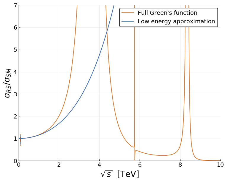
If we raise the center-of-mass energy further, the behavior of our approximate formula (47) will eventually deviate from that of the full Green’s function (93), which includes resonances from gauge KK states at masses of a few . Fig. 1 shows an example of how the cross section predictions differ between the approximate formula (blue line) and the full Green’s function (orange line) for processes. The vertical axis shows the size of the cross section compared to that of the SM prediction and we used TeV for this plot. We can see that both lines start at but deviate near . The KK resonances appear near 4, 6, and 8 TeV in the full Green’s function. The good agreement between the two lines show that our formula (47) is indeed an excellent approximation in the region of our interest, 250 GeV 1 TeV. We will study the process more in detail in Section 5.
4.2 Pair-production of UV-localized fermions
The simplest case to which we might apply the formulae in the previous section is that of light fermions whose zero-mode wavefunctions are strongly localized near the UV boundary.
For a UV-localized final state, as implied by (50). Then and are the only quantum numbers relevant in the process . That is, we find the same cross section regardless of how we embed those light flavors into an multiplet.
For the contact interactions, we find
| (51) |
which are suppressed by . The cross section deviations from these terms and the other terms with are small enough to satisfy any current precision constraints on the light flavors. For TeV, our formulae predict KK recurrences of the photon and with masses above 3.5 TeV. These resonances also have suppressed couplings to UV-localized zero mode fermions.
The most direct bound on from the LHC is that from constraints on contact interactions. The strongest lower bound now quoted for a scale in contact interactions is 40 TeV (25 TeV for destructive interference), for a universal left-handed interaction, from the ATLAS experiment at 13 TeV [20]. Translating the limit TeV into that of using (47), we obtain TeV. This is not yet as strong as the constraint from precision electroweak measurments.
5 Mass generation and pair-production for the quark
In this section, we study schemes of mass generation for the bottom quark and their implications for the cross section for . The strong top Yukawa coupling and the large mass separation between the top and bottom quark restrict how the bottom quark is embedded into an multiplet.
We assume that the generation of the top quark mass is the main driving force of the electroweak symmetry breaking. To achieve this, the Higgs field must couple with full strength to the top quark. This implies that the 5D multiplet containing the doublet must also contain the , so that the two chirality states of the top quark are directly linked by the the Higgs field . Furthermore, the parameter of the top quark multiplet should not be much bigger than so that it can couple strongly to the Higgs field. We consider the range in our analysis.
If were also included in the top quark multiplet, it would gain the same mass from electroweak symmetry breaking as the top quark. To otain a much smaller mass for the quark, we need to place the in a different multiplet and postulate a flavor mixing between this 5D multiplet and the top quark multiplet that assists the Higgs field to connect the and . We model this mixing by an -invariant mixing of the two multiplets on the UV brane, parametrized by .
It follows from this setup that the assignment of the is directly given by that of the top quark, and that the assignment of is specified almost uniquely once we choose the representation of its 5D multiplet. In this paper, we consider two choices, and of .
5.1 in the 5 of
In [4], we assigned the mutiplet that contains the multiplet to the 5 of . This follows the suggestion by Agashe, Contino, Da Rold, and Pomerol that this choice provides a custodial symmetry constraining the coupling [21, 22]. We found that this choice also has quantitative advantages in fitting the mass of the Higgs boson [4]. We can also embed the into a different 5 multiplet .
More specifically, we embed the top and bottom quarks as
| (52) |
We will denote the 5D mass parameters of the two multiplets as and , respectively. In (52), the matrix in parentheses is a bidoublet, with acting vertically and acting horizontally. The fields and have electric charge and , respectively. The signs in parentheses indicate the UV and IR boundary conditions for each field. The and fields contain right-handed zero modes. The notation denotes mixing on the UV brane, as we will now explain.
For the left-handed zero mode and fields, we define the combinations
| (53) |
and assign definite boundary conditions
| (54) |
Note that and have the same and the same , so the mixing is invariant. The contain left-handed zero modes. Note that and must be assigned opposite UV boundary conditions; otherwise the mixing has no effect. This construction allows the Higgs field, which acts only within an multiplet, to connect and , generating a quark mass.
We also include the UV boundary kinetic term for the doublet, so that we can adjust this parameter to obtain the correct top quark mass for any values of . The details of the formalism of the fermion UV boundary kinetic term can be found in [4].
In the limit where the effect is a small perturbation, the mass of the top quark is determined by the four model parameters: , , , and . The mass of the quark depends on the two additional parameters , and . The full formulae for the and masses are given in Appendix C. We will quote here the simplifications of these formula using and .
The top quark mass is given by
| (55) |
with
| (56) |
For , , similar to in (12). For our choice of parameters, the logarithm equals 4.61, and we need values of in the range 5–9 to fit the observed top quark mass [4]. A large value of pulls a large fraction of the and wavefunctions to the UV brane and so decreases the observable RS effects on cross sections. Keeping the top quark mass fixed as , and are varied requires a compensatory variation of , and this affects the predictions of the theory, as will be apparent below. The boundary kinetic term must have a positive coefficient, so we will restrict ourselves to the region where for our phenomenological discussion.
Using the same approximations, the mass ratio between the top and bottom quark is given by
| (57) |
The relation (57) shows us that there are two independent strategies to realize the correct ratio. First, we can choose a small UV mixing angle . Second, we can choose , giving a suppression that is exponential in this difference. The first mechanism is rather intuitive, but the second is not. It works because the field is pushed to the UV, minimizing its overlap with the . This same parameter choice pushes the right-handed zero mode in the to IR, increasing its degree of compositeness.
In computing the effects of the mass generation on the cross sections, we find that the explicit effects of are of order , parametrically smaller than the effects described above. Once we have understood the ranges of , expected from the mass generation mechanism, we can ignore explicit effects of and in the calculation of cross sections. This also allows us to ignore the term in (48).
With this choice of assignments, for both and . Then, the parameter in (48) equals zero up to ignorable matrix elements of . We will see the implication of this for the cross sections in Section 5.3.
5.2 in the 4 of
Another possibility is to embed the top and bottom quarks in the 4 of [23],
| (58) |
The notation for boundary conditions is the same here as in (52), and again we represent the and mixing by (53) and (54). The formulae for the top and bottom quark masses in this case are also worked out in Appendix C. The final result for the mass ratio is again (57). So, also in this case, we need small or to obtain the correct mass ratio between the top and bottom quarks.
With this embedding, we now have nonzero :
| (59) |
We can relate to the top quark mass since resides in the same multiplet with and . As shown in Appendix C, the relation is
| (60) |
for small and . As a representative value, for TeV and . Note that its dependence on is weak. Although the value of is small, the presence of nonzero is strongly constrained by pole precision measurements. We will show now that embedded in 4 of is unfavored.
In [4], we studied the constraints on the RS wavefunctions of the and in the 5 arising from the values at the resonance of , the fraction of hadronic decays to , and , the polarization asymmetry in . The value of is very accurately known [24],
| (61) |
The correction to is given by
| (62) |
where are fractional deviations of . This is dominated by the correction to the coupling because of the small size of the SM coupling to ,
| (63) |
The constraints on and from are much weaker.
In RS models of the type we are describing, there are three contributions to , arising, respectively, from , and in (48). In [4], we showed that contributions from the first two sources lead to effects that are much smaller than the experimental error in (61). For in the 5, this is the end of the story. For in the 4, is nonzero and (61) leads to the bound
| (64) |
which excludes the value of found above. The effect of strengthens this bound. Including this effect, values TeV are needed to be consistent with our precision knowledge of .
However, the possibility is still open to embed in the 5 but in the 4. We can mix the of in (52) with the of in (58), and generate the bottom quark mass. In this case, the formula for the mass ratio becomes
| (65) |
This makes only a minor change in the overall logic. In this case, is identically zero. The bound on is weaker than that quoted above due to the suppression factor . With , we have
| (66) |
This should be compared to the formula (48),
| (67) |
This formula contains as the prefactor rather than as in (60); the coefficient is larger by a factor of . Computing for , we have
| (68) |
Then we find at , at . This is a significant constraint but one that allows most of the parameter space of interest to us.
5.3 Deviations of the pair-production cross section
We can now assess the effects of the RS structure on the cross sections for . In the approximation in which we ignore the quark mass, the leading order cross sections for completely polarized beams take the form
| (69) |
The terms , are associated with the production of ; the terms , are associated with the production of . At a linear collider with polarized beams and using vertex charge to distinguish and , all four of these functions can be measured independently at a fixed [25].
As we have explained in the previous section, the cross sections in RS models will differ from those computed in the SM through the effects parametrizd by and in (48). We consider first the case in which both the and the are assigned to 5 representations of . Here for both chiral states of the quark, and so for both and . The visible effects of the RS structure then come only from the contact term induced by the gauge KK states.


Fig. 2 shows cross section deviations of the process for in the 5 of . The upper graph refers to beams, and the lower graph to beams. The horizontal and vertical axes in the upper plot show the cross section deviations
| (70) |
and, similarly, the axes of the lower plot give the deviations in and . The central black line show the effect on these cross section contributions as the center of mass energy is varied from 250 GeV to 1 TeV for the choice of parameters
| (71) |
The additional parameters of the model are fixed from the precision electroweak measurements, including the masses of the and , and, to fix , the mass of the top quark. The added lines show the effect of varying the parameters in (71) individually, from 0.3 to 0.6 for and , and from 0.1 to 0.13 for . It should be noted that is always positive in this range of parameters. Finally, the dashed lines show deviations for TeV. Increasing decreases the effects uniformly as .
In this case with , the deviations are almost zero at small , but increase with as the contact interaction becomes more dominant. With the positive value of , the is very composite and gives larger values for the moments in . As an example, the value of for is larger for than for by a factor of , as shown in (50). This is reflected in the ratio of the vertical to the horizontal scales on the plot. The increasing makes the more composite, and it makes larger. The situation for is more subtle. One might guess that increasing makes the less composite and therefore decreases the effect on the cross section. However, according to (55), increasing at fixed top quark mass requires a decrease in the value of . This is actually a larger effect in the opposite direction that makes the wavefunction larger at large values of . This leads to larger cross section deviations, as shown in the figure. Similarly, increasing requires larger , and this decreases the cross section deviation for .
In the two graphs in Fig. 2, we show our estimate of the 68% confidence region for measurements of the two cross sections and the two cross sections that would be obtained at the International Linear Collider (ILC) at 250 GeV with 2 ab-1 of data. This estimate is based on results presented in the study [25]. It will be difficult to discern these cross section deviations at 250 GeV, though they will become apparent at higher center of mass energies.
Consider next the case in which the is assigned to the 5 of while the is assigned to the 4. Now is nonzero. The effect of on , is largest on the pole and decreases as we increase the center-of-mass energy. This leads to a different pattern of deviations for the cross sections for production.


Fig. 3 shows the cross section deviations for this case, using the same notation as that used in Fig. 2. We see that is already sizable at GeV, enough so to be readily observed at the 250 GeV ILC. As we go away from the pole, the effect of decreases and the contact term becomes more dominant. This explains the non-monotonic behavior of as is increased. Also note that is not suppressed with larger (dashed lines) at small , since does not depend on directly.
It is interesting to see that the sign of the the effect of changes between the and the initial state. To understand this, look back at (47). Due to the small coupling of , the photon propagator is dominant over the propagator for final state. According to (48), is negative. In (47), the term with is multiplied by , which is negative for and positive for . Comparing to the photon propagator term, this contributes constructively for and destructively for , in accord with the results displayed in the Fig. 3.
Although Figs. 2 and 3 include only slices of the paramter space, they allow us a detailed understanding of how each parameter affects the cross section. They also demonstrate that the two cases have physically distinct predictions and can be distinguished by precision experiments. The most important effect appears in the backward cross section for beams, so both beam polarization and excellent separation is needed to observe and separate the predicted effects.
6 Pair-production of the quark
In this section, we compute the pair production cross section for the top quark. In the calculations of the previous section, we made strong use of the fact that the bottom quark mass is much smaller than the new physics scale and the center-of-mass energy even at 250 GeV. This allowed us to ignore the effect of the mass in the pair production cross section. However, for the massive top quark, we must take the nonzero quark mass into account. This does not change the calculation conceptually, but it adds more bookkeeping that must be carried out correctly.
6.1 Cross section calculation for the top quark
The calculation of the cross section adds four new elements. First, the mass of the top quark cannot be ignored, and so both the left- and right-handed chirality states of the top quark must be included. Second, each top quark chirality state is a part of a 5D field that is a Dirac fermion, and so, both for and , the full 4-component Dirac fermion must be accounted. Third, the operator in (40) and (48), which has nonzero matrix elements between the and Dirac fermions, must now be taken into account. Finally, the final states have four possible helicity states, so (69) must now be enlarged to
In this equation, the LL and RL terms are associated with the production of the helicity (not chirality) state , the RL and RR terms are associated with the production of the helicity state , and the L0 and R0 terms are associated with the production of the helicity states and . In the models discussed in this paper, the latter two helicity amplitudes are equal by .
One more possible complication does not appear. The 5th components of the gauge fields have couplings of the form with nonzero matrix elements between the left- and right-chirality components of the 5D fermion fields. However, as we noted already in Section 2, our use of the Feynman-Randall-Schwartz gauge [14] implies that, since the massless electron does not couple to the fields, the diagrams in which the fields couple to the top quark are zero.
To compute the amplitudes for , we must first construct the and wavefunctions, and then take the matrix elements between these wavefunctions of the propagator (47). In the model, with and assigned to the 5 of , the and belong to the multiplet in (52). After breaking, the and mix with one another, and with a third field, the in (52). In Appendix D, we construct the propagator for these three fields and use it to extract the top quark wavefunctions. It turns out that the component of this wavefunction containing is of order . In the cross section calculation, the overlaps between this term and other terms in the wavefunction have additional suppression by powers of . So, we can ignore the contribution in this calculation.
The wavefunction of the top quark can then be written in terms of the left- and right-chirality components of the Dirac fields and . In the Dirac basis in which is diagonal, write a massive Dirac spinor with mass , spin and momentum as
| (73) |
Similarly, the spinor of an antifermion is
| (74) |
where , , and denotes the flipped spin [26]. Then, ignoring , working to order , and ignoring small terms from the mixing, we show in Appendix D that the physical top quark wavefunction takes the form
| (75) |
The functions and are the left- and right-handed zero mode wavefunctions defined in (14) and (17). The kets in the brackets denote the quantum numbers of the corresponding Dirac fields. The expressions for the coefficients are given in Appendix D. It should be noted that each of the chiral wavefunctions is separately normalized. For example, for the left-chirality term, this implies (for simplicity, setting )
| (76) |
We can now compute the neutral gauge boson propagator between states of definite helicity for and in the initial state and states of definite helicity for and in the final state. The first step is to take the matrix element of (47) between the partial wavefunctions in brackets in (75). The operators ( are the pure numbers and , respectively, acting on and in (75), and that mediates between and ,
| (77) |
without changing the chirality. For , in (48) receives a nonzero contribution from the first term in parentheses proportional to . For both and , there is a nonzero contribution from the second term, proportional to , where the second factor comes from the wavefunction overlap between the opposite chirality components.
Finally, we compute the overlaps of the final-state spinors. For example, for , where the and now refer to physical top quark and antiquark helicity eigenstates,
| (78) |
and for , again, for the physical helicity eigenstates,
| (79) |
where are the final energy and momentum of the top quarks. Assembling all of the pieces, we find expressions for the helicity-dependent differential cross sections in the form ().
6.2 Deviations of the pair-production cross section
We now present the numerical values for the deviations of the helicity cross sections for from the predictions of the SM. Since we have seen in Section 5.2 that the case of in the 4 of is disfavored by the constraint from , we will only consider here the case of in the 5.
In our discussion of the quark cross sections, the term in (48) gave the dominant effect at low energies. Thus we predicted relatively small corrections to the SM for in the 5 where but large corrections for in the 4. In the top quark case, is nonzero, though it has a different origin. Specifically,
| (80) |
For , the moment is suppressed, since is partially elementary when . On the other hand, in the same range of , is highly composite, leading to a quite significant contribution.
Enhancement of the and cross sections is the standard signal of an anomalous top quark magnetic moment induced by new physics [27]. In this class of models, however, the enhancements of these cross sections are not especially large.


Fig. 4 shows the cross section deviations for the and helicity states, in a presentation similar to that of Fig. 2. The central values of the parameters are again taken to be those in (71). The added lines show the effect of varying the parameters in (71) individually, from 0.3 to 0.6 for , from 0.1 to 0.13 for , and, finally, with the dashed lines, from to TeV. In the two graphs in Fig. 4, we show our estimate of the 68% confidence region for measurements of the two cross sections and the two cross sections that would be obtained at the International Linear Collider (ILC) at 500 GeV with 4 ab-1 of data. These estimates are based on results presented in the study [28]. Both the and effects should be seen clearly for beams given the expected accuracy of the measurements. Fig. 5 shows the cross section deviations in the helicity-flip final states or .


7 Conclusions
In this paper, we have present general formulae for the helicity-dependent cross sections for and in a broad class of RS models with fermions and gauge bosons in the bulk and bulk gauge symmetry. Through an analytic understanding of the corrections to the electroweak propagators induced by the RS structure, we have been able to understand intuitively when this structure predicts sizable corrections to the SM expectations that might be visible in precision experiments. Indeed, the precision measurement of even at 250 GeV in the center of mass can discriminate the models that we have discussed. Thus, these measurements can open a new window into the dynamics of composite Higgs models even at the initial energy of the ILC.
In the processes we discuss in this paper, the largest effects appear in subdominant helicity states. These can be recognized in the cross sections using beam polarization and the high degree of discrimination between and that linear collider experiments make possible. We hope that our analysis will be useful to those who plan for these features in future experiments.
ACKNOWLEDGEMENTS
We are grateful to Kaustubh Agashe, Yutaka Hosotani, Marcel Vos, and our colleagues in the SLAC Theory Group for useful discussions and advice. We are especially grateful to Roman Pöschl for pushing us to closely examine the physics of production at colliders. This work was supported by the U.S. Department of Energy under contract DE–AC02–76SF00515. JY is supported by a Kwanjeong Graduate Fellowship.
Appendix A Treatment of wavefunctions in the presence of boundary kinetic terms
In our discussion of the fermion zero mode wavefunctions, we saw that the inclusion of a boundary kinetic term creates a singular part of the wavefunction at that contains a finite fraction of the normalization integral. In this appendix, we describe how we can compute and work with such wavefunctions without needing to deal explicitly with the singular terms.
First, we can compute the regular part of the wavefunction from the propagator. This is in fact the way that we derived the expression (14) and similar expressions for gauge field wavefunctions in Appendix C of [4]. We first compute the Green’s functions for the fields that give rise to the particle, using the rules explained in that Appendix that account for the boundary kinetic term. Then we notice that, on the particle pole, these Green’s functions factorize into the form
| (81) |
The resulting wavefuntion is correctly normalized acording to a prescription such as (15) that includes the boundary kinetic term.
This calculation gives only the smooth part of the wavefunction at . However, that smooth wavefunction will correctly compute expectation values of functions that vanish at . Since the wavefunction is normalized when its singular term is included, expectation values of general functions can be computed using a generalization of the formula (16).
Appendix B Neutral gauge field propagator
In [4], we constructed the low-energy limit of the Green’s function for the neutral gauge bosons in the model. Here we present an alternative, and somewhat more transparent, derviation of the expression for this Green’s function in the limit that we require for this paper.
In Appendix E of [4], we presented the following representation for this Green’s function: For ,
| (82) |
and are diagonal matrices of functions which satisfy the UV and IR boundary conditions, respectively. The expression (82) makes intuitive sense; it satisfies the correct boundary conditions on each of the two branes, and it has the correct poles in , which must appear at the zeros of . In the basis defined in (38) and (40), we have and take the form
| (83) |
and
| (84) |
where we have used the abbreviation , and similarly for .
The Wilson line element (42) has the form
| (85) |
and the C maxtrix is given by , where and are the UV boundary condition of the field and the IR boundary conditions of the field, respectively. Explicitly,
| (86) |
The determinant of C is
| (87) |
To evaluate (82), we need the inverse of C. However, note that, if the initial fermion states are extremely UV-localized, as we assume for the electrons in , then we will evaluate at . In this case, the third and fourth rows of involve only , so they are identically zero. Then we only need to work out the first two rows of , or, equivalently, the first two columns of . We find that these can be written in the relatively simple form
| (88) |
where
| (89) |
For the reaction , the RS form factor defined in (20) and (21) takes the form
| (90) |
where
| (91) |
We can evaluate this expression using the decomposition (88), to find
| (92) |
where
| (93) | |||||
We can get some insight into this expression by computing its low energy approximation. To do this, we expand the functions for small and ,
| (94) |
neglecting terms of order .
The first zero of is identified with the boson mass. The location of this zero is at such that
| (95) |
where and , defined in terms of model parameters in (46). Similarly,
| (96) |
Appendix C Top and bottom quark masses
In this appendix, we compute the top and bottom quark masses from poles of their Green’s functions. The poles are determined by zeros of the determinant of C matrix[4], which is given by , where and are the UV boundary condition of the field and the IR boundary conditions of the field, respectively. correpsponds to the UV mixing matrix with angle defined in (53).
We first consider the embedding (52) in 5 of . In the basis , the C matrix for the top quark is
| (98) |
where and . and are evaluated at with the mass parameter and , respectively. We will write explicitly at points of possible confusion between the mass parameter and . The determinant of the matrix is given by
| (99) |
In the basis , the C matrix for the bottom quark is
| (100) |
The determinant of the matrix is given by
| (101) |
The top and bottom quark masses correspond to the first zeros of the two determinant (99) and (101). To show the explicit leading order expression of the top and bottom mass, it is convenient to define
| (102) |
Then, we have
| (103) |
Then the ratio of the two masses is given by
| (104) |
and for and postivie and , it reduces to (57).
Similarly, we can compute the masses of the top and bottom quark in the 4 of , defined in (58). The determinants of the are given by
Note that and are identical up to the difference in and . The top and bottom quark masses in 4 are
| (106) |
The mass ratio is identical to (104).
We can proceed similarly for mixed representation case, that is, in 5 and in 4 of . The calculation of in this case gives from (103) and from (106). Then for the mass ratio, we have
| (107) |
for small .
It is interesting to compute how in (59) is related to the top quark mass. Note that we are interested in the range and therefore it is a good approximation to ignore terms with and . Then, the mass of the top quark in 4 is
| (108) |
where we neglect the small effect of mixing. Also, if we compute the expectation value with in (14) and (15), we have
| (109) |
Then, for small , we have
| (110) |
as in (60).
Appendix D The wavefunction of the quark in the model
In this Appendix, we construct the on-shell quark wavefunction. We compute the propagator of the multiplet in (52), and identify quark wavefunction from the quark pole terms. Some clarification of the notation is necessary.
The details of computing fermion Green’s functions in RS spacetime is again given in [4]. Here we simply quote essential results. The Green’s functions of fields obeying boundary conditions on the IR brane (therefore, in UV gauge) is given by
| (112) |
The Green’s functions , , and are constructed similarly, with for each .
The top quark pole is contained in the matrix . After electroweak symmetry breaking, the physical top quark is a mixture of the three fields , , in (52). We ignore the effect of the UV mixing with the multiplet, since it is always of higher order in our approximation. In the basis , the matrix A is given by where
| (113) |
and
| (114) |
Note that we use .
More explicitly, we can write
| (115) |
where
| (116) |
and
| (117) |
with .
The first zero of gives the top quark pole . Then, on the pole, we have an identity
| (118) |
where functions are evaluated at . Using this identity, one can show that the factorizes onto the pole of a single fermion
| (119) |
where
| (120) |
From , we can write
| (121) |
The expression for will be given below. Now we are ready to construct the full wavefunction of the physical quark. From (112), (120), and (121), the left-handed chirality wavefunction of the top quark is given by
| (122) | |||||
where is 2-component projection of a massive spinor onto left-handed chirality. The right-handed chirality wavefunction is given by replacing and .
We can expand the top quark wavefunction up to the first corrections in or . It will be useful to adopt a compact notation for the expansions of the functions. We will write
| (123) |
and similarly for the other functions, putting the appropriate subscript on the coefficient.
Note that component is suppressed by . In the pair production process, the top quark wavefunction always appear as its square, and therefore the contribution of can be ignored. Then we have
where
| (125) |
and
| (126) |
We have made the above formulae somewhat simpler by ignoring factors of and (but not ) for the relevant values . Note the difference in sign of coefficients compared to those defined in Appendix G of [4], since we are working in the Minkowski space.
References
- [1] B. Bellazzini, C. Csáki and J. Serra, Eur. Phys. J. C 74, no. 5, 2766 (2014) [arXiv:1401.2457 [hep-ph]].
- [2] C. Csaki, C. Grojean and J. Terning, Rev. Mod. Phys. 88, no. 4, 045001 (2016) [arXiv:1512.00468 [hep-ph]].
- [3] J. Yoon and M. E. Peskin, Phys. Rev. D 96, 115030 (2017) [arXiv:1709.07909 [hep-ph]].
- [4] J. Yoon and M. E. Peskin, arXiv:1810.12352 [hep-ph]].
- [5] L. Randall and R. Sundrum, Phys. Rev. Lett. 83, 3370 (1999) [hep-ph/9905221].
- [6] L. J. Hall, Y. Nomura and D. Tucker-Smith, Nucl. Phys. B 639, 307 (2002) [hep-ph/0107331].
- [7] M. Kubo, C. S. Lim and H. Yamashita, Mod. Phys. Lett. A 17, 2249 (2002) [hep-ph/0111327].
- [8] R. Contino, Y. Nomura and A. Pomarol, Nucl. Phys. B 671, 148 (2003) [hep-ph/0306259].
- [9] K. Agashe, R. Contino and A. Pomarol, Nucl. Phys. B 719, 165 (2005) [hep-ph/0412089].
- [10] S. Funatsu, H. Hatanaka, Y. Hosotani and Y. Orikasa, Phys. Lett. B 775, 297 (2017) [arXiv:1705.05282 [hep-ph]].
- [11] F. Richard, arXiv:1403.2893 [hep-ph].
- [12] D. Barducci, S. De Curtis, S. Moretti and G. M. Pruna, JHEP 1508, 127 (2015) [arXiv:1504.05407 [hep-ph]].
- [13] See, for example, T. Gherghetta, in Physics of the Large and Small (Proceedings of TASI 2009), C. Csaki and S. Dodelson, eds. (World Scientific, 2011). [arXiv:1008.2570 [hep-ph]].
- [14] L. Randall and M. D. Schwartz, JHEP 0111, 003 (2001) [hep-th/0108114].
- [15] W. D. Goldberger and M. B. Wise, Phys. Rev. D 60, 107505 (1999) [hep-ph/9907218].
- [16] H. Davoudiasl, J. L. Hewett and T. G. Rizzo, Phys. Rev. Lett. 84, 2080 (2000) [hep-ph/9909255], Phys. Lett. B 473, 43 (2000) [hep-ph/9911262].
- [17] T. Gherghetta and A. Pomarol, Nucl. Phys. B 586, 141 (2000) [hep-ph/0003129], Nucl. Phys. B 602, 3 (2001) [hep-ph/0012378].
- [18] Y. Grossman and M. Neubert, Phys. Lett. B 474, 361 (2000) [hep-ph/9912408].
- [19] P. Sikivie, L. Susskind, M. B. Voloshin and V. I. Zakharov, Nucl. Phys. B 173, 189 (1980).
- [20] M. Aaboud et al. [ATLAS Collaboration], JHEP 1710, 182 (2017) [arXiv:1707.02424 [hep-ex]].
- [21] K. Agashe, R. Contino, L. Da Rold and A. Pomarol, Phys. Lett. B 641, 62 (2006) [hep-ph/0605341].
- [22] R. Contino, L. Da Rold and A. Pomarol, Phys. Rev. D 75, 055014 (2007) [hep-ph/0612048].
- [23] K. Agashe and R. Contino, Nucl. Phys. B 742, 59 (2006) [hep-ph/0510164].
- [24] S. Schael et al. [ALEPH and DELPHI and L3 and OPAL and SLD Collaborations and LEP Electroweak Working Group and SLD Electroweak Group and SLD Heavy Flavour Group], Phys. Rept. 427, 257 (2006) [hep-ex/0509008].
- [25] S. Bilokin, R. Pöschl and F. Richard, arXiv:1709.04289 [hep-ex], and R. Pöschl, personal communication.
- [26] M. E. Peskin and D. V. Schroeder, An Introduction to Quantum Field Theory (Westview Press, 1995), Chapter 3.
- [27] G. L. Kane, G. A. Ladinsky and C. P. Yuan, Phys. Rev. D 45, 124 (1992).
- [28] M. S. Amjad et al., Eur. Phys. J. C 75, 512 (2015) [arXiv:1505.06020 [hep-ex]].