The leading non-renormalizable interactions describing semi-leptonic decays $d_{i}\to u_{j}$ below the electro-weak scale is given by the low-energy effective Hamiltonian

where $V$ is the CKM matrix and

are the four-fermion vector, scalar and tensor operators, respectively, $P_{X}$ with $X=\{L,R\}$ are the fermionic chiral projector to the left-handed (LH) and right-handed (RH) field components, $u$, $d$ and $\ell$ are the generic up-quark, down-quark and charged leptons fields for which we have omitted the flavor indices and $g_{\!\,{}_{I}}$ with $I\in\{V_{L},S_{X},T\}$ are the Wilson coefficients.

We now specialize to the semi-tauonic $b\to c$ transitions and fit the coefficients $g_{\,V_{X},\,S_{X},\,T}$ to $R_{D^{(*)}}$ assuming negligible NP contributions to $b\to c\,(e,\mu)\bar{\nu}$ decays. In Fig. 1 (left), we show results of the one-parameter fits to each Wilson coefficient at the scale $m_{b}$. The dashed portion of the curves correspond to the exclusion limits from the $B_{c}$ lifetime on the branching ratio of $\text{Br}(B_{c}\to\tau\nu)<30\%$ [13, 14]. The only single operator that can explain the charged current anomaly is $\mathcal{O}_{V_{L}}$ (red curve) with $V-A$ structure. The tensor operator $\mathcal{O}_{T}$ can also fit the anomaly, but nonetheless is always generated in combination with scalar operators after integrating out the heavy NP state (see for example [15]). The anomaly can be successfully accommodated by scalar and tensor operators with Wilson coefficients satisfying $g_{S_{L}}=\pm\,4g_{T}$ at the NP scale (taken her at $\mu=1$ TeV). As shown in Fig. 1 (right) [11], after running from the TeV scale down to $m_{b}$ we obtain one real solution (blue curve) and one imaginary solution (cyan curve) that fit very well $R_{D^{(*)}}$. Here, and through out this paper, we omit operators with light RH neutrinos. For these type of models the reader is referred to [16, 17, 18, 19].

In order to explore NP above the electro-weak breaking scale, it is necessary to restore the full SM gauge symmetry and work with the SM effective field theory (SMEFT) framework. In the Warsaw basis [20], the complete set of dimension-6 operators giving rise to semi-leptonic $d_{i}\to u_{j}$ transitions are given by:

Here $Q_{i}=(V^{*}_{ji}u^{j}_{L},d_{L}^{i})^{T}$ and $L_{i}=(U_{ji}^{*}\nu^{j}_{L},\ell_{L}^{i})^{T}$ are the LH quark and lepton doublets in the basis aligned with diagonal down-quarks and charged leptons, $U$ is the $3\times 3$ PMNS mixing matrix for neutrinos and $[C_{I}]$ with $I\in\{V_{L},S_{X},T\}$ are the Wilson coefficients. Interestingly, because of $\mathrm{SU}(2)_{L}$ invariance, these operators, besides giving rise to charged current transitions $d^{i}\to u^{j}\ell^{k}\nu^{k}$ will also generate neutral current transitions of the form $u^{i}\bar{u}^{j},d^{i}\bar{d}^{j}\to\ell^{k}\ell^{l}$. We now need to fix the flavor structure in (6). A reasonable assumption is to impose a global flavor symmetry $U(2)_{q_{1,2}}\times U(2)_{\ell_{1,2}}$ acting non-trivially on the first two generations [21]. In the limit this symmetry is exact, one is left only with third generation currents $[C_{I}]_{ijkl}=\delta_{i3}\delta_{j3}\delta_{k3}\delta_{l3}\,C_{I}$. The necessary couplings between different quark generations arise through CKM mixing. Notice that the results we present here should not change much if this global $U(2)^{2}$ symmetry is slightly broken. Once electro-weak symmetry is spontaneously broken, an immediate consequence of this flavor structure is the appearance of flavor diagonal transitions $t\to b$ and neutral currents $b\to b$, $t\to t$ that are $V_{cb}^{-1}$ enhanced with respect to the $b\to c$ transitions for $R_{D^{(*)}}$. Of particular interest are the potentially large BSM contributions to $b\bar{b},c\bar{c}\to\tau\bar{\tau}$ scattering [10]. Indeed, since the characteristic scale of NP lies below the TeV scale and the neutral current couplings must be of order $\mathcal{O}(1)$ this opens the possibility for directly searching for the NP responsible for $R_{D^{(*)}}$ in $\tau\bar{\tau}$ Drell-Yan production at the LHC. As we show bellow, a close look a the existing LHC data in the $\tau\bar{\tau}$ tails exclude some of the standard proposals solving the $R_{D^{(*)}}$ anomaly, namely, the vector $W^{\prime}$ boson and the charged scalar $H^{+}$.

LQs have recently gained attention as possible solutions to the $B$-anomalies. Out of the 12 possible LQ states [24] respecting the SM gauge symmetry, only a few can explain the anomalies. The current status of these models is described in Table 1, see Ref. [11] for more details. There are three minimal scenarios that solve the $B$-anomalies: (i) one vector $U_{1}$ [25] or two pairs of scalars (ii) $R_{2}$ and $S_{3}$ [12] and (iii) $S_{1}$ and $S_{3}$ [29, 25]. The relevant simplified models for each of these scenarios are described below (we do not include here the simplified model for $S_{3}$ LQ since it has a small impact on LHC phenomenology). On a side note, UV completions for these three LQ scenarios have been proposed in the literature. For example, in Refs. [26, 27] $U_{1}$ is the Pati-Salam gauge boson of the $\mathrm{SU}(4)$ gauge group. In [12, 28], $R_{2}$ and $S_{3}$ come from an $\mathrm{SU}(5)$ GUT framework, while in [30] $S_{1}$ and $S_{3}$ are taken as pseudo Nambu-Goldstone modes from a strongly coupled theory.

We now confront the simplified models with $pp\to Z^{\prime}\to\tau\bar{\tau}$ resonance searches at the LHC. Constraints were first derived in [10] using both 8 TeV and 13 TeV ATLAS searches in the hadronic tau category at $20$ fb^-1[34] and $3.2$ fb^-1 [35], respectively. One important result from this study is that color-neutral NP models for $R_{D^{(*)}}$ with perturbative couplings, i.e. $W^{\prime}$ and $H^{\prime}$, are excluded by $\tau\bar{\tau}$ data. Results for the vector triplet are given in Fig. 3 (left), where we show the $95\%$ CL upper limits for fixed values of $g_{V_{L}}=|g_{b}g_{\tau}|v^{2}/M^{2}_{Z^{\prime}}$ as red iso-contours in the mass versus width plane of the $Z^{\prime}$ boson. The allowed region in green (yellow) accommodates the $R_{D^{(*)}}$ anomaly at $1\sigma$ ($2\sigma$). This shows that the width of the $Z^{\prime}$ boson must be unnaturally broad, surpassing 30-40%, in order to evade these direct search limits. Similar conclusions can be reached for the neutral scalar and pseudoscalar $H^{0}/A^{0}$.

For LQ models the limits from recasting di-tau resonance searches are evidently much weaker. For example, for the vector $U_{1}$ LQ the $95\%$ CL exclusion limits in the coupling²² 2 In the plot we have redefined the coupling to $g_{U}\equiv x^{b\tau}_{L}$. vs mass plane shown in Fig. 3 (right) is given by the gray region (red region) for the 13 TeV (8 TeV) LHC searches. Notice that the LHC is starting to probe the green band that explains the $B$-anomaly at $1\sigma$ for LQ couplings in the limit of exact $U(2)^{2}$ flavor symmetry. A naive projection of these limits to a higher luminosity of $300$ fb^-1 shows that the LHC will completely probe this scenario. Nonetheless, as shown in [25], explicitly breaking the global $U(2)^{2}$ symmetry by allowing for a (small) non-zero $x^{s\tau}_{L}$ coupling in (11) leads to a reduction of $x^{b\tau}_{L}$ in the $R_{D^{(*)}}$ fit. This particular scenario evades these di-tau bounds and gives motivation for future HL-LHC studies. In fact, a more recent $\tau\bar{\tau}$ search by ATLAS [36] at a luminosity of $36.1\penalty\ \mathrm{fb}^{-1}$ was used in [11] to update the $3.2\penalty\ \mathrm{fb}^{-1}$ limits on both vector and scalar LQs. In Fig. 4 we provide the $95\%$ CL exclusion limits in the coupling $y^{q\ell}$ ($x^{q\ell}$) vs mass plane for several scalar (vector) LQs and different initial sea quarks, $b\bar{b}\to\tau\bar{\tau}$ (solid blue), $c\bar{c}\to\tau\bar{\tau}$ (solid green) and $s\bar{s}\to\tau\bar{\tau}$ (solid red). Similarly, we have also included in dashed lines and the same color code, the exclusion limits from recasting a $Z^{\prime}$ resonance search by ATLAS [37] in di-muon tails at $36.1\penalty\ \mathrm{fb}^{-1}$ for $t$-channel LQ exchange in $pp\to\mu\bar{\mu}$. While these bounds are not relevant for the $R_{D^{(*)}}$ anomaly, the di-muon tails can be constraining for certain NP models for $R_{K^{(*)}}$ at tree-level [38] and very constraining for one-loop models for $R_{K^{(*)}}$ [39].

The most relevant LQ process at the LHC is pair production $gg\,(q\bar{q})\to\text{LQ}^{\dagger}\text{LQ}$. ATLAS and CMS have searched for this process in different decay channels into second and/or third generation quarks and leptons, $\mathrm{LQ}^{\dagger}\mathrm{LQ}\to q\bar{q}\ell\bar{\ell},\,q\bar{q}\nu\bar{\nu}$. As a result, these searches lead to useful model independent bounds on both the mass and branching fractions of the LQ. For example, the vector $U_{1}$ LQ in the exact $U(2)^{2}$ flavor limit, when produced in pairs decays into $c\bar{c}\nu\nu$ and $b\bar{b}\tau\tau$ each with a 25% branching ratio. The best limit on the mass is currently at $M_{U}>1.5$ TeV from a LQ search by CMS for final state dijets plus missing energy. In Table 2 we list the most recent lower limits on the masses of second/third generation scalar and vector LQs relevant for the $B$-anomalies, for benchmark branching ratios set to $\beta\!=\!1\,(0.5)$. For more details on LQ pair searches see [11, 26].

Besides pair production and $t$-channel Drell-Yan production, LQs can also be singly produced at the LHC via $qg\to\text{LQ}\,\ell,\,\text{LQ}\,\nu$. This mode is usually sub-dominant for small LQ couplings to fermions and only becomes important when the couplings are large enough, usually for LQ couplings above $y^{q\ell},\,x^{q\ell}\sim 2$. Interestingly, given that non-resonant Drell-Yan LQ production, LQ pair production and single LQ production all scale differently with powers of the LQ coupling, implies that all three modes give complementary bounds in parameter space, as illustrated in Fig. 5 in Ref. [45]. For this reason all modes should be thoroughly searched by both experimental collaborations at the LHC.

This LQ model equipped with a minimally broken $U(2)^{2}$ global symmetry is the only single particle³³ 3 Declared Particle of the Year at CKM 2018. able to generate $R_{K^{(\ast)}}<R_{K^{(\ast)}}^{\mathrm{SM}}$ and $R_{D^{(\ast)}}>R_{D^{(\ast)}}^{\mathrm{SM}}$ while respecting all low energy flavor and LHC constraints. To explore this in more detail, we assume for the $U_{1}$ Lagrangian in (10) the following generic structure for the Yukawa matrices:

An important observation from Fig. 5 is that in order to avoid the current $\tau\bar{\tau}$ bounds from LHC a non-zero (small) value for $|x_{L}^{s\tau}|$ is necessary. In addition to this, the requirement of non-vanishing $x_{L}^{s\mu}$ and $x_{L}^{b\mu}$ to explain the $R_{K^{(*)}}$ anomaly have an important impact on the LFV decays in this model, in particular the modes $B\to K\mu\tau$ and $\tau\to\mu\phi$. This has been illustrated in Fig. 6. Notice that the projected LHC bounds lead to a lower bound for each of these modes of order $\mathcal{O}(10^{-7})$ for $\mathrm{Br}(B\to K\mu\tau)$ and $\mathcal{O}(10^{-11})$ for $\mathrm{Br}(\tau\to\mu\phi)$. We have also included the current bounds from BaBar [47] and by Belle [48] for each LFV mode (solid hashed lines). We see that lowering the upper bound on $\mathrm{Br}(B\to K\mu\tau)$ and $\mathrm{Br}(\tau\to\mu\phi)$ at the LHCb and/or Belle II can have a major impact on the model building by further restraining the parameter space. Here, for definiteness we focus on $B\to K\mu\tau$, but the discussion would be completely equivalent if we used $B_{s}\to\mu\tau$ or $B\to K^{\ast}\mu\tau$, because their branching fractions are known to be related.

A simultaneous solution to the $B$-anomalies can arise from a UV complete model based on $\mathrm{SU}(5)$ Grand Unified Thoery (GUT), where two light scalar LQs, $R_{2}$ and $S_{3}$, appear at the TeV scale [12]. Once integrated out, the doublet gives rise to the Scalar/Tensor operators explaining $R_{D^{(*)}}$ while the triplet generates the $V-A$ operator necessary for explaining $R_{K^{(*)}}$. Furthermore, $S_{3}$ and $R_{2}$ have a common origin in the UV given that both states are (partially) embedded in the same scalar representation $\bf 45$ of $\mathrm{SU}(5)$. As a consequence, at low energies both LQs share the same Yukawa matrix, $y_{L}$, up to a sign. We now focus on $R_{2}$ since it drives the phenomenology at the LHC. Once rotating Eq. (15) to the mass eigenbasis, the simplest flavor texture for this model is

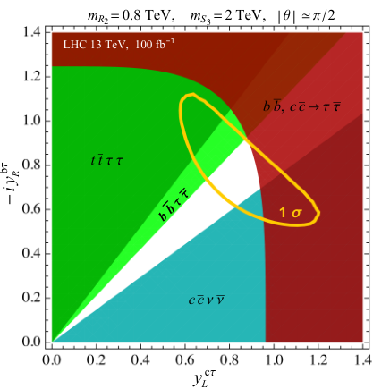
where $\theta$ is a mixing angle, $s_{\chi}\equiv\sin\chi$, $c_{\chi}\equiv\cos\chi$, $y_{R}^{b\tau}$ is a complex Yukawa coupling and both $y_{L}^{c\mu}$ are $y_{L}^{b\tau}$ are real Yukawa couplings. These 4 parameters along with the two LQ masses are the total six parameters of this model. As a benchmark for the LHC analysis we set $m_{2}=800$ GeV (and $m_{S_{3}}=2$ TeV). In Fig. 7 (left) we show in red (orange) the $1\sigma$ ($2\sigma$) region from a global fit to all relevant low energy observables in the complex plane of the scalar Wilson coefficient $g_{S_{L}}=4g_{T}$. We also included in the same figure the $2\sigma$ regions accommodating $R_{D}$ in purple and $R_{D^{*}}$ in blue. The low energy fit requires the mixing angle to satisfy $\sin^{2}(2\theta)\approx 0$, leading to two possible solutions $\theta\approx\{0,\pi/2\}$. Interestingly, the current limit for the LFV observable $\mathrm{Br}(\tau\to\mu\phi)$ breaks this degeneracy and fixes the mixing angle to be near maximal, i.e. $\theta\approx\pi/2$.

To finilize, we now confront this model to the direct searches at the LHC. The main contributions to di-tau production come from the $t$-channel exchange of the components $R_{2}^{(5/3)}$ and $R_{2}^{(2/3)}$ in $c\bar{c}\to\tau\bar{\tau}$ and $b\bar{b}\to\tau\bar{\tau}$, respectively⁵⁵ 5 Sub-leading contributions from the more massive $S_{3}$ to $b\bar{b}\to\tau\bar{\tau}$ have also been included in this analysis. These effects are negligible at the LHC.. Our results for the 95% CL limits in the $y_{L}^{c\tau}$–$(y_{R}^{b\tau}/i)$ plane are given by the red exclusion region in Fig. 7 (right) at a projected LHC luminosity of 100 fb^-1 for the benchmark masses and $|\theta|\approx\pi/2$. Since the $R_{2}$ LQ needs to be quite light, we also took into account bounds from pair production. To set these limits we used the CMS search [40] targeting $pp\to(R_{2}^{(2/3)})^{*}R_{2}^{(2/3)}$ decaying into $b\bar{b}\tau\bar{\tau}$ final states and the multi-jet plus missing energy search [44] for decays into $c\bar{c}\nu\bar{\nu}$ final states. The 95% CL exclusion limits are shown by the light green and turquoise regions in Fig. 7 for a luminosity of 100 fb^-1. As for pair produced $R_{2}^{(5/3)}$ states decaying into $t\bar{t}\tau\bar{\tau}$ we employed Ref. [41]. This result corresponds to the dark green exclusion region in Fig. 7 (right). The $1\sigma$ region satisfying all low-energy data, including the $B$-anomalies, is given in the same figure by the thick yellow contour. Interestingly, for such a low $R_{2}$ mass there is still allowed parameter space, which could eventually be covered by the HL-LHC. Notice that for a slightly higher masses of $\approx 1$ TeV the LHC pair production bounds relax considerably. In this model we have also found a complementarity between high energy and low energy observables. In particular, between high-mass di-tau tails, the rare decay $\text{Br}(B\to K\nu\bar{\nu})$ and the LFV decay mode $\text{Br}(B\to K\mu\tau)$, for more details see [12]. Experimental inputs from HL-LHC, Belle II and LHCb could ultimately test the predictions for these observables in the near future. Another interesting prediction, which is a consequence of the almost purely imaginary coupling $y_{R}^{b\tau}$, is a new source of CP violation. See for instance [49] for a recent analysis of the current and projected limits from electric dipole moment searches.

References

- [1] J. P. Lees et al. [BaBar Collaboration], Phys. Rev. Lett. 109 101802 (2012),
- [2] J. P. Lees et al. [BaBar Collaboration], Phys. Rev. D 88 no. 7 072012 (2013)
- [3] M. Huschle et al. [Belle Collaboration], Phys. Rev. D 92 no. 7 072014 (2015)
- [4] R. Aaij et al. [LHCb Collaboration], Phys. Rev. Lett. 115 no. 11 111803 (2015), Erratum: [Phys. Rev. Lett. 115 no. 15 159901 (2015)]
- [5] S. Hirose et al. [Belle Collaboration], Phys. Rev. Lett. 118 no. 21 211801 (2017)
- [6] Y. Sato et al. [Belle Collaboration], Phys. Rev. D 94 no. 7 072007 (2016)
- [7] A. Abdesselam et al. [Belle Collaboration], arXiv:1603.06711
- [8] R. Aaij et al. [LHCb Collaboration], Phys. Rev. Lett. 113 151601 (2014)
- [9] R. Aaij et al. [LHCb Collaboration], JHEP 1708 055 (2017)
- [10] D. A. Faroughy, A. Greljo, J. F. Kamenik, Phys. Lett. B 764 126 (2017), arXiv:1609.07138
- [11] A. Angelescu, D. Bečirević, D. A. Faroughy, O. Sumensari, JHEP 1810 (2018) 183, arXiv:1808.08179
- [12] D. Bečirević, I. Doršner, S. Fajfer, D. A. Faroughy, N. Košnik, O. Sumensari, Phys. Rev. D98 (2018) no.5 055003, arXiv:1806.05689
- [13] X. Q. Li, Y. D. Yang, X. Zhang, JHEP 1608 054 (2016), arXiv:1605.09308
- [14] R. Alonso, B. Grinstein, J. M. Camalich, Phys. Rev. Lett. 118 no. 8 081802 (2017), arXiv:1611.06676
- [15] M. Freytsis, Z. Ligeti, J. T. Ruderman, Phys. Rev. D 92 no. 5 054018 (2015), arXiv:1506.08896
- [16] Bečirević et al., Phys. Rev. D94 (2016) 11 115021 arXiv:1608.08501.
- [17] A. Greljo, D. J. Robinsonan, B. Shakya, J. Zupan, JHEP 1809 (2018) 169, arXiv:1804.04642.
- [18] P. Asadi, M. R. Buckley, D. Shih, JHEP 1809 (2018) 010, arXiv:1804.04135
- [19] D. J. Robinsonan, B. Shakya, J. Zupan, arXiv:1807.04753.
- [20] B. Grzadkowski, M. Iskrzynski, M. Misiak, J. Rosiek, JHEP 1010 (2010) 085, arXiv:1008.4884.
- [21] A. Greljo, G. Isidori, D. Marzocca, JHEP 1507 (2015) 142, arXiv:1506.01705.
- [22] D. Pappadopulo, A. Thamm, R. Torre, A. Wulzer, JHEP 1409 060 (2014), arXiv:1402.4431
- [23] G. Abbiendi et al. [ALEPH and DELPHI and L3 and OPAL and LEP Collaborations], Eur. Phys. J. C 73 2463 (2013), arXiv:1301.6065
- [24] I. Doršner, S. Fajfer, A. Greljo, J. F. Kamenik and N. Košnik, Phys. Rept. 641 1 (2016), arXiv:1603.04993
- [25] D. Buttazzo, A. Greljo, Gino Isidori, D. Marzocca, JHEP 1711 (2017) 044, arXiv:1706.07808
- [26] B. Diaz, M. Schmaltz, Y. M. Zhong, JHEP 1710 097 (2017), arXiv:1706.05033
- [27] L. Di Luzio, A. Greljo, M. Nardecchia, Phys. Rev. D 96 no. 11 115011 (2017), arXiv:1708.08450; N. Assad, B. Fornal, B. Grinstein, Phys. Lett. B 777 324 (2018), arXiv:1708.06350; M. Bordone, C. Cornella, J. Fuentes-Martin, G. Isidori, Phys. Lett. B 779 317 (2018), arXiv:1712.01368; L. Calibbi, A. Crivellin, T. Li, arXiv:1709.00692; M. Blanke, A. Crivellin, Phys. Rev. Lett. 121 no. 1, 011801 (2018), arXiv:1801.07256; R. Barbieri, A. Tesi, Eur. Phys. J. C 78 no. 3 193 (2018), arXiv:1712.06844; A. Greljo, B. A. Stefanek, Phys. Lett. B 782 131 (2018), arXiv:1802.04274
- [28] I. Doršner, S. Fajfer, D. A. Faroughy, N. Košnik, JHEP 1710 188 (2017), arXiv:1706.07779
- [29] A. Crivellin, D. Müller, T. Ota, JHEP 1709 040 (2017), arXiv:1703.09226
- [30] D. Marzocca, JHEP 1807 (2018) 121, arXiv:1803.10972
- [31] D. Bečirević, B. Panes, O. Sumensari, R. Zukanovich Funchal, JHEP 1806 032 (2018), arXiv:1803.10112
- [32] Y. Sakaki, M. Tanaka, A. Tayduganov, R. Watanabe, Phys. Rev. D 88 no. 9 094012 (2013), arXiv:1309.0301
- [33] G. Hiller, D. Loose, K. Schönwald, JHEP 1612 (2016) 027, arXiv:1609.08895
- [34] G. Aad et al. [ATLAS Collaboration], JHEP 1507 157 (2015) arXiv:1502.07177
- [35] M. Aaboud et al. [ATLAS Collaboration], Eur. Phys. J. C76 (2016) 11 585, arXiv:1608.00890
- [36] M. Aaboud et al. [ATLAS Collaboration], JHEP 1801 055 (2018), arXiv:1709.07242
- [37] M. Aaboud et al. [ATLAS Collaboration], JHEP 1710 182 (2017), arXiv:1707.02424
- [38] A. Greljo, D. Marzocca, Eur. Phys. J. C 77 no. 8 548 (2017), arXiv:1704.09015
- [39] J. E. Camargo-Molina, A. Celis, D. A. Faroughy, Phys. Lett. B 784 (2018) 284-293, arXiv:1805.04917
- [40] A. M. Sirunyan et al. [CMS Collaboration], JHEP 1707 121 (2017), arXiv:1703.03995
- [41] A. M. Sirunyan et al. [CMS Collaboration], arXiv:1803.02864
- [42] CMS Collaboration [CMS Collaboration], CMS-PAS-EXO-17-003
- [43] CMS Collaboration [CMS Collaboration], CMS-PAS-B2G-16-027
- [44] CMS Collaboration [CMS Collaboration], CMS-PAS-SUS-18-001
- [45] I. Doršner, A. Greljo, JHEP 1805 (2018) 126, arXiv:1801.07641
- [46] F. Feruglio, P. Paradisi, A. Pattori, Phys. Rev. Lett. 118 no. 1 011801 (2017), arXiv:1606.00524; F. Feruglio, P. Paradisi, A. Pattori, JHEP 1709 061 (2017), arXiv:1705.00929; C. Cornella, F. Feruglio, P. Paradisi, arXiv:1803.00945
- [47] J. P. Lees et al. [BaBar Collaboration], Phys. Rev. D 86 (2012) 012004, arXiv:1204.2852
- [48] Y. Miyazaki et al. [Belle Collaboration], Phys. Lett. B 699 (2011) 251, arXiv:1101.0755
- [49] W. Dekens, J. De Vries, M. Jung, K. K. Vos, arXiv:1809.09114.