MIMO Channel Information Feedback Using Deep Recurrent NetworkManuscript received October 29, 2018; accepted November 15, 2018. This work of was supported by NSFC under grants 61871109, 61871108 and 61601115, the Six Talent Peaks project in Jiangsu Province under GDZB-005, the Natural Science Foundation of Jiangsu Province under BK20150635, and the Royal Academy of Engineering under the Distinguished Visiting Fellowship scheme. The editor coordinating the review of this paper and approving it for publication was Dr. G. A. Baduge.(Corresponding authors: Wei Xu, Hong Shen.) C. Lu, W. Xu and H. Shen are with the National Mobile Communications Research Laboratory, Southeast University, Nanjing, China ({220170709, wxu, shhseu}@seu.edu.cn). J. Zhu is with the Qualcomm Incorporated, San Diego, CA, USA (junzhu@qti.qualcomm.com). K. Wang is with the Department of Computer and Information Sciences, Northumbria University, Newcastle, UK (kezhi.wang@northumbria.ac.uk).
Abstract
In a multiple-input multiple-output (MIMO) system, the availability of channel state information (CSI) at the transmitter is essential for performance improvement. Recent convolutional neural network (NN) based techniques show competitive ability in realizing CSI compression and feedback. By introducing a new NN architecture, we enhance the accuracy of quantized CSI feedback in MIMO communications. The proposed NN architecture invokes a module named long short-term memory (LSTM) which admits the NN to benefit from exploiting temporal and frequency correlations of wireless channels. Compromising performance with complexity, we further modify the NN architecture with a significantly reduced number of parameters to be trained. Finally, experiments show that the proposed NN architectures achieve better performance in terms of both CSI compression and recovery accuracy.
Index Terms:
Channel state information (CSI) feedback, recurrent neural network (RNN), multiple-input multiple-output (MIMO).I Introduction
As a key technology in 5G, massive multiple-input multiple-output (MIMO) has become a focus in both academia and industry in recent years. Massive MIMO has shown superior performance in terms of system capacity, energy efficiency, and anti-interference capability. In order to reap the performance gain, it is critical to obtain channel state information (CSI) accurately at the transmitter.
In massive MIMO communications, the number of antennas at the base station (BS) is usually large, and thus the overhead of downlink pilots and uplink CSI feedback can be quite high. The conventional codebook based method quantizes the CSI into a number of bits [1]. However, it can fail to achieve satisfactory performance since it can not linearly increase the performance with the quantization bits owing to its exponentially increasing complexity.
Recently, neural network (NN) has shown great potentials in addressing some wireless communication challenges which are naturally nonlinear problems [2, 3]. Deep learning based methods have achieved remarkable progress in the field of MIMO channel quantization and feedback. By treating MIMO channel matrix as an image, the network, namely CsiNet in [4], adopted trendy image processing network architectures, e.g., ResNet [5], for MIMO CSI compression and feedback.
In this letter, we propose a new NN by incorporating recurrent neural network (RNN) to catch the temporal channel correlation. Compared to the parallel work in [6], which also exploits RNN to enhance the network in [4], our work focuses on the design of feature compression and uncompression modules while [6] considers enhancing the channel recovery module. The compression and uncompression modules in [4] and [6] both utilize linear fully-connected networks (FCN), which are not sufficiently effective especially in tracking the temporal correlations in compression.
The main contributions of this work are summarized as follows:
- •
We develop a deep NN using modules with memory for CSI compression and feedback in MIMO communications. Recurrent compression and uncompression modules are designed to exploit the channel correlation effectively. The performance is significantly improved compared to existing methods.
- •
We further devise a method to reduce the training complexity. The number of parameters in the network reduces sharply while the performance advantage still retains.
II CSI Compression and Feedback
Consider a frequency division duplexed (FDD) MIMO downlink with antennas at the BS and a single antenna at each user equipment (UE). The received signal at the th subcarrier can be expressed as:
| (1) |
where represents the channel response at the th subcarrier, denotes the precoding vector at the th subcarrier, denotes the modulated data symbol, and is the additive noise. An estimate of is assumed to be acquired at each UE. Then, the channel is quantized with a codebook and the quantization information is sent back to the BS for CSI recovery [1]. However, the codebook based quantization may fail to fully exploit the sparsity nature of channels since the quantization have to catch the amplitude and phase of every path in finite number of codewords. Additionally, the size of codebook grows exponentially with the number of quantization bits which can cause large storage and computational overhead. Different from the codebook based method, the NN is able to compress the CSI within short time and achieve high performance [4]. Thus, in our study, we consider the application of NN, which follows the design philosophy previously proposed in [4].
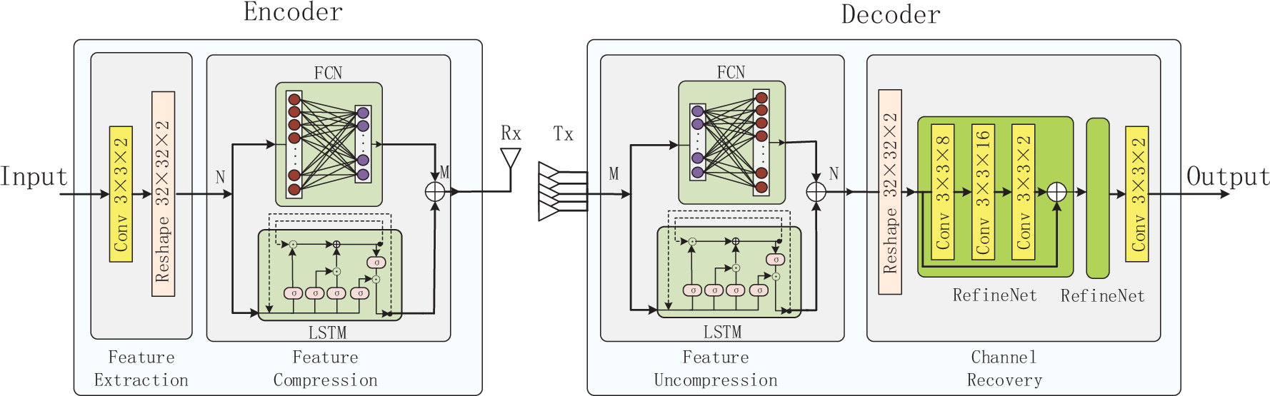
In Fig. 1, we depict the NN based CSI compression and feedback model. For the ease of tractability as in [4], the channel is first transferred into the angular-delay domain by 2D discrete Fourier transform (DFT) before being processed by the NN. Let be the channel information in the angular-delay domain, where denotes the number of subcarriers. For the convenience of NN processing, is separated into real and image parts, and all the entries are normalized within [0,1]. Instead of using codebook based CSI quantization, is compressed through an “Encoder” which is realized via a deep NN. It compresses the input of CSI estimate into a few bits which are then fed back to the BS. After getting the full-bit information, a “Decoder” at the BS recovers the CSI using another deep NN. The output size of the Encoder and the input size of the Decoder are both set to . The number of the elements of the cropped channel is denoted by . Parameter represents the channel information compression ratio.
The existing Encoder design of CsiNet in [4] employs a convolutional filter and uses the leaky rectified linear unit (LeakyRELU) as the nonlinear activation function before a linear FCN to complete CSI compression. On the other side, a linear FCN and two RefineNet modules followed by a convolutional layer constitute the Decoder. The RefineNet consists of 3 convolution operations and a jump connection. According to the basic module of ResNet [5], this architecture promises the stability of the network and helps restore the channel information effectively.
Since the channel varies slowly in many typical massive MIMO applications [7], the correlation within a sequence of channel information can be explored for more efficient CSI compression. In the following section, we propose a new design of Encoder and Decoder architectures by introducing modules with memory. Different from CsiNet, the extracted features are compressed by taking, e.g., temporal correlation, into account. Correspondingly, the proposed Decoder block at the BS also exploits the temporal correlation for CSI sequence recovery. Mathematically, let , where denotes the -th entry of the th channel matrix in the channel sequence, denotes the standard Gaussian random variable and is the absolute value function. The correlation between adjacent CSI inputs is represented by .
III Proposed CSI Neural Network with Memory
In this section, we describe the design details of our proposed NN involving compression and uncompression modules with memory.
III-A Recurrent Compression and Uncompression Modules
In this subsection, we modularize the Encoder and Decoder architecture in the proposed NN.
As depicted in Fig. 1, Encoder contains two modules. The feature extraction module mainly extracts channel features through convolution operations. The feature compression module then compresses the features. Correspondingly, Decoder also has two main modules. The feature uncompression module is responsible for recovering compression features and the recovery module then restores the channel matrix.
To be more specific, the feature extraction module employs a convolutional filter, which is referred from CsiNet [4], while the recovery module utilizes two RefineNets and a convolutional layer. The compression and uncopression modules are proposed using the long short-term memory (LSTM) network [8], which has the memory function and thus can capture and extract inherent correlations, e.g. temporal correlations within input sequences. In our design, see Fig. 1, the input of the compression module is split into two parallel flows: an LSTM network and a linear FCN. The FCN serves as a jump connection which can accelerate the convergence and reduce the vanishing gradient problem [5]. The input size of the compression module is while the output size is , typically . Since it projects the size from to , we can add the two flows together at the output end. In the proposed NN architecture, we let the LSTM network learn the residual features, instead of learning correlation features directly, which is more robust.
Correspondingly at the BS, the uncompression module includes two flows which are realized by a linear FCN and an LSTM network, respectively. The only difference between the compression and uncompression modules is the input and output sizes, which needs to be symmetric.
According to [8], the architecture in LSTM is shown in Fig. 2 and the computations involved in the LSTM are:

| (2a) | |||
| (2b) | |||
| (2c) | |||
where and denote the input and the output of the LSTM cell, respectively. The computations of and are almost the same as [8]. and serve as the weight parameters and the corresponding bias parameters, respectively. Here denotes the Hadamard product. and are nonlinear activation functions.
The LSTM network is usually used for sequence modeling, due to its ability to capture correlation [8]. This can be verified through Eq. (2): is determined by its previous state and the present input . The amount of information kept and forgotten by LSTM is determined by the learned parameters. This memory mechanism enables LSTM to compress the temporal redundancy. Regarding the training complexity, the compression and uncompression modules occupy the majority of the total parameters to be trained in our proposed NN. As for the convolutional operation, it only has 18 parameters, which is ignorable. Considering the parameters at the UE in Fig. 1, the FCN has parameters. The parameters of the LSTM is made up of and . The sizes of , and are and , respectively. Thus the number of parameters at the BS amounts to . Similarly, the amount of training parameters of the NN at the UE is of the same order of magnitude. Note that, in deep learning networks, gated recurrent unit (GRU) is an alternative of LSTM for modeling sequences with memory. In our proposed NN architecture, the LSTM can be replaced by GRU without much additional changes to our current design.
III-B Recurrent Compression and Uncompression Modules with Reduced Complexity
The above proposed recurrent CsiNet, referred to as RecCsiNet, suffers from the problem of a large number of training parameters. Here, we provide a far more effective solution to address this issue. The parameter-reduced recurrent CsiNet (PR-RecCsiNet) utilizes new compression and uncompression modules as illustrated in Fig. 3. We use a linear FCN to project -dimensional input to -dimensional output and the output size of LSTM is reduced to in the uncompression module. Therefore, the parameter size of the uncompression module at the BS reduces to . Another benefit of this projection is to force the LSTM to have the same input and output size. Consequently, the jump connection on the LSTM does not need any dimension transformation before the addition operation. The same modifications are correspondingly made in the compression module.
Comparing the proposed architectures in Fig. 1 and Fig. 3, RecCsiNet connects LSTM and FCN in parallel while PR-RecCsiNet connects LSTM and FCN in serial. The FCN in the two networks play different roles. FCN in RecCsiNet serves as a jump connection with dimension transformation between the input and output of LSTM. In PR-RecCsiNet, the input and output of LSTM already have the same size, which allows us to link them together directly. The FCN projection in PR-RecCsiNet is designed to reduce the training parameter size of the network by reducing the input size of LSTM.
Since the input size of the LSTM cell is reduced, the parameter size of the network is reduced notably. As we can see in Table I, the parameter size of RecCsiNet is about 19M while the parameter size of PR-RecCsiNet is reduced to 0.8M at compression ratio 1/16. With the involvement of the projection layer, the parameter size of our recurrent network, as compared in Table I, remains comparable with that of the existing techniques, e.g., CsiNet and CsiNet-LSTM. Since FCN compresses the features extracted from the channel matrix to a lower dimension, it could bring some information loss compared to RecCsiNet.

IV Numerical Results
In this section, we describe the detailed setup of our experiments and compare our method with existing methods. The values of are generated based on the COST2100 [9] and mmWave [10, 11] channel models. The sequence length is set to 4 for convenience. The BS uses antennas and subcarriers. Since the multipath arrivals are limited to short adjacent time slots around the direct path, only the first rows of are non-zeros. Thus we reserve the first rows of the channel .
All the networks are trained end-to-end by using the criterion of minimizing the mean squared error (MSE). The loss function is expressed as:
| (3) |
where and denote the parameters of Encoder and Decoder. and denote the network functions of Encoder and Decoder. is the th step of the th sample, is the start index of the mini-batch, denotes the batch size, and is the sequence length. The training, validation and testing sets have 100,000, 30,000 and 20,000 sequences, respectively. The correlation factor is identical in the training, validation and testing sets. We keep in CsiNet-LSTM [6] for a fair comparison, which implies that CsiNet-LSTM feeds back the same size of codewords in every step. Results for both unquantized and quantized codewords are given. For the quantized version, we add a “tanh” function to map all the elements to (-1,1) before the codewords are fed back, and then divide the interval uniformly by 8 bits. Thus the codeword can be replaced by a 8-bit sequence. To compare with the conventional AoD codebook based method [1], we test two cases with 8 bits and 16 bits for each main path. The compression ratios of the networks are accordingly set to 1/64 and 1/32.


NMSE is used as the performance metric which is defined as , where denotes the expectation operation and denotes the Frobenius norm. Fig. 4 shows the performance of RecCsiNet at compression ratio of 1/16. When the correlation coefficient increases, the channel temporal correlation decreases, and thus the NMSE grows correspondingly. Fig. 5 illustrates the NMSE performance at different time steps. It can be seen that the NMSE of our networks drops noticeably before convergence as the temporal correlation appears.

| AoD codebook[1] | CsiNet [4] | PR-RecCsiNet | RecCsiNet | |
|---|---|---|---|---|
| 8 bits/path | -7.69 | -10.55 | -11.54 | -12.02 |
| 16 bits/path | -9.56 | -13.99 | -16.34 | -17.21 |
Fig. 6 gives the NMSE performance of recent deep learning methods under COST 2100 channel model. is set as the x-axis for convenience. The proposed RecCsiNet shows noticeable advantages under various compression ratios. CsiNet-LSTM shares similar performance gains as RecCsiNet at some compression ratios. However, the parameter size of CsiNet-LSTM is almost five times that of ours as compared in Table I. The parameter size of the proposed PR-RecCsiNet reduces sharply, while the performance beats CsiNet. The proposed PR-RecCsiNet can be considered as a promising option in a memory and computation limited application. Table II gives the comparison of quantized versions under mmWave channels, which shows that our networks still outperform the conventional methods.
Furthermore, we also compare the time complexity of these methods. Since there exists no GPU solution for the codebook based method, we test it on an i7-6800k CPU, and all other network based methods are tested on a Nvidia GTX 1080Ti GPU. The average processing time of AoD codebook based method is 320 ms under 8 bits/path, while CsiNet, RecCsiNet, PR-RecCsiNet and CsiNet-LSTM require 0.1 ms, 0.9 ms, 0.6 ms and 1.1 ms, respectively, when the compression ratio is 1/64. The time complexity of all the networks is almost the same, which is far less than the AoD codebook based method.
V Conclusion
We have proposed a new network architecture and proposed recurrent compression/uncompression modules to exploit the time-varying features in an effective manner. Apart from this, we have also provided a simple method to reduce the parameter size. In the letter, we limit ourselves to the design of the compression and uncompression modules. By further optimizing the feature extraction module and the channel recovery module, we expect that the encoder-decoder NN will achieve a better performance. Moreover, a direct extension to multi-user MIMO mandates assigning a Decoder Network for each user at the BS separately. Ongoing effort focuses on a more compact and integral design needs further investigation.
References
- [1] W. Shen et al., “Channel feedback based on AoD-adaptive subspace codebook in FDD massive MIMO systems,” IEEE Trans. Commun., Jun. 2018, early access.
- [2] C. Lu et al., “An enhanced SCMA detector enabled by deep neural network,” in Proc. ICCC, Beijing, China, Aug. 2018, pp. 161–165.
- [3] T. J. O’Shea and J. Hoydis,“An introduction to deep learning for the physical layer,” arXiv preprint arXiv:1702.00832, 2017.
- [4] C. K. Wen, W. T. Shih, and S. Jin, “Deep learning for massive MIMO CSI feedback,” IEEE Wireless Commun. Lett., Mar. 2018, early access.
- [5] K. He et al. “Deep residual learning for image recognition,” arXiv preprint arXiv:1512.03385, 2016.
- [6] T. Wang et al., “Deep learning-based CSI feedback approach for time-varying massive MIMO channels,” arXiv preprint arXiv:1807.11673, 2018.
- [7] H. Ji, G. Zaharia, and J. Hélard, “Performance of DSTM MIMO systems in continuously changing Rayleigh channel,” in Proc. ISSCS, Iasi, Jul. 2015, pp. 1–4.
- [8] K. Greff et al., “LSTM: A search space odyssey,” IEEE Trans. Neural Netw., vol. 28, no. 10, pp. 2222–2232, Oct. 2017.
- [9] L. Liu et al., “The COST 2100 MIMO channel model,” IEEE Wireless Commun., vol. 19, no. 6, pp. 92–99, Dec. 2012.
- [10] “Spatial channel model for multiple input multiple output (MIMO) simulations,” 3GPP TR 25.996, 2009.
- [11] “Study on channel model for frequencies from 0.5 to 100 GHz simulations,” 3GPP TR 38.901, 2018.