Optimal Quantum Subtracting machine
Abstract
The impossibility of undoing a mixing process is analysed in the context of quantum information theory. The optimal machine to undo the mixing process is studied in the case of pure states, focusing on qubit systems. Exploiting the symmetry of the problem we parametrise the optimal machine in such a way that the number of parameters grows polynomially in the size of the problem. This simplification makes the numerical methods feasible. For simple but non-trivial cases we computed the analytical solution, comparing the performance of the optimal machine with other protocols.
pacs
03.67.-a, 03.67.Ac, 03.65.Ta.I Introduction
A fundamental fact in quantum information theory is that not all maps between quantum states are possible: even before considering practical difficulties, quantum theory itself limits the operations that can be performed. A series of quantum no-go theorems Wootters1982; WERNER; KumarPati2000; PhysRevLett.116.110403; dieks1982communication; PhysRevLett.100.090502; Noprogramming; QA2 shows that transformations which would be very valuable from the point of view of information processing are in fact impossible. The most celebrated of them is the no-cloning theorem Wootters1982: the impossibility of cloning makes many processing tasks (e.g. state estimation) non-trivial. Nonetheless, the importance of these impossible transformations drives the search for approximate implementations of them: optimal cloners RevModPhys.77.1225 have been extensively studied, and similar efforts have been spent for other no-go theorems QA2; PhysRevLett.116.110403; PhysRevA.96.052318; PhysRevA.97.052330; Sepehr.
Here we introduce the no-subtracting theorem, which states the impossibility of undoing the mixing operation that involves a target state we wish to recover and an external noise source, and define the optimal subtractor operation which solves the problem with the best allowed approximation. This task is somehow related to those discussed in ReviewFramesInfo and references therein, where one aims to perform quantum information processing of some sort (e.g. the recovery of the target state) when some classical knowledge (i.e. the reference frame for ReviewFramesInfo and the amount of mixed noise for us) is replaced by bounded information encoded into the density matrix of an ancillary quantum system. Finding the optimal subtractor corresponds to a semidefinite program involving a number of variables that in principle grows exponentially with the input data (system copies). However, by exploiting the symmetry of the problem and a proper parametrisation of the to 1 qubit covariant channels (analogous to those introduced in Refs. ResourceAsymmetry; longevitycovariant), the number of effective parameters can be reduced to a subset which only scales polynomially. This reduction of the parameters makes the numerical optimisation feasible, and for small enough input data, allows also for analytical treatment.
As a final consideration we would also to point out that the problem we address in the present paper can also be seen as an instance of quantum machine learning QM1; QM2; QM3, an emerging area of quantum information theory that deals with tasks that generalise the “learning from example” concept in a genuine quantum information theory setting. In these tasks a machine should be trained to perform a certain quantum operation and this training can be done through quantum processing, that means with quantum training data and quantum operations. The fundamental difference with classical training tasks is that there is not an a priori separation between the training and the execution phases, because of entanglement. Indeed, in our analysis we search for the best machine that can be trained with copies of the noise in order to make it able to recover disturbed signals, with the only requirement that the machine is allowed by quantum mechanics.
The paper is organized as follows: we start in Sec. II by formalizing the problem. In Sec. III we present some preliminary results on the efficiency of a universal quantum subtractor which can drawn from general consideration on the problem without passing the explicit optimization stage. In Sec. IV we then proceed with the explicit solution of the optimization problem. The paper ends with Sec. V. Technical derivations are presented in the Appendix.
II Optimal Subtractor
An Universal Quantum Subtracting machine UQS is a two-inputs/one-output transformation acting on two isomorphic quantum systems A and B. When provided by factorised input states of the form , with assigned and arbitrary density matrices, it returns as output the system A into the state realizing the mapping
| (1) |
which effectively allows one to recover from the mixture by “removing” the perturbing state and renormalizing the result. Unfortunately the possibility of physically realizing an UQS machine for , turns out to be in contradiction with the basic requirements that any quantum evolution has to fulfil, see e.g. Ref. HOLEVOBOOK. Indeed invoking linearity and using the fact that for one has , Eq. (1) can be cast in the following form
| (2) |
which, as long as the parameter is strictly different from 0, will produce unphysical non-positive results as soon as the support of admits a non trivial overlap with the kernel of . Yet, as in the case of other better studied impossible quantum machines WERNER, there could be still room for approximate implementations of the mapping (1). In what follows we shall hence try to identify the implementation of an optimal UQS, i.e. a machine which, being physically realizable via a Completely Positive and Trace Preserving (CPTP) map HOLEVOBOOK, would give us the best approximation of the transformation (1). More generally we are also interested in a generalisation of the problem where instead of a single copy of the mixture and of the noise state , we are now provided with copies of the first and copies of the second, i.e. in the optimal CPTP implementation of the mapping
| (3) |
As a figure of merit we shall consider the fidelity DEP1 between the obtained output and the intended target states, properly averaged with respect to all possible inputs. To simplify the analysis in what follows we restrict ourself to the special case where both and are pure states of the -dimensional space , namely and , where without loss of generality we adopt the parametrisation and , with being a fixed vector and , are arbitrary elements of the unitary set . Indicating hence with the CPTP mapping that we want to test as a candidate for the implementation of , we evaluate its performance through the function
| (4) |
where the integral are performed via the Haar measure of to ensure a uniform distribution of and on . Before entering into the technical derivation, it is worth commenting that while the problem we are facing can be seen as a sort of purification procedure, it is definitely different from the task addressed by Cirac et al. in Ref. CIRAC, which is designed to remove the largest fraction of complete mixed state from having access to some copies of it, but with no prior information on or .
II.1 Connection to Quantum Error Correction
Equation (1) can be described as the formal inversion of the transformation
,
which we may dub Incoherent Quantum Adder.
At variance with the Coherent Quantum Adder analyzed in Refs. QA2; PhysRevA.96.052318; PhysRevA.97.052330, an IQA can be easily implemented as it merely consists in creating a probability mixture out of two input configurations.
In particular, IQA can be interpreted as an open quantum evolution HOLEVOBOOK; DEP1; DEP2 in which the state of the input B, plays the role of the environment. In this scenario, the aim is to undo the action of IQA and recover not having the full knowledge about the environment, the only information available being encoded through copies of .
In view of this observation the optimal quantum subtracting problem can be seen as a first example of a new way of approaching quantum error correction schemes.
We are thinking for instance to communication scenarios where, the transformation tampering the received
state at the output of the channel is affected by interactions with an external environment E that
is susceptible to modifications on which the communicating parties (say Alice and Bob) do not have a complete record. To be more precise, imagine the following realistic situation where Alice uses a noisy channel to communicate with Bob. Therefore, the states that Alice wants to send to Bob , interacts with the environment . The coupling Hamiltonian between the information carrier and E and the transfer time of the communication are somehow fixed and known. while the state of the environment is not – is a sort of
a random, possibly time-dependent variable of the problem.
Accordingly, Bob receives by
with and being the
partial trace over E.
The fundamental task for the receiver of the message is clearly to recover from :
in the standard approach to quantum communication this is facilitated by the assumption that Alice and Bob
have also perfect knowledge about which in our setting is no longer granted.
To compensate for this lack of information it is hence important for the receiver of the message to sample the state of E
in real time during the information exchange, a scenario which we can model e.g. by assuming Bob to
have access to some copies of .
The optimal subtracting scheme we discuss in the manuscript addresses
exactly this problem for the special (yet not trivial) case where describes a partial swap gate (see e.g. scarani3
).
Given the above premise it should be now clear that the possibility of constructing an UQS machine will have a profound impact in many practical applications, spanning from
quantum computation QCOMP; DEP1, where it could be employed as an effective error correction procedure for certain kind of errors,
to quantum communication QCOM, where instead it could be used as a decoding operation to
distill the intended messages from the received deteriorated signals.
III Preliminary results
The maximum of Eq. (4) with respect to all possible CPTP transformations
| (5) |
is the quantity we are going to study in the following. Since one can always neglect part of the input copies, this functional is clearly non-decreasing in and , i.e.
| (6) |
with no ordering between the last two terms been foreseen from first principles. In particular, we are interested in comparing with the performances achievable via a trivial “doing nothing” (DN) strategy in which one emulates the mapping (3) by simply returning as output one of the qubits of the register A, i.e. the state . In this case, the associated average fidelity can be easily computed by exploiting the depolarizing identity
| (7) |
obtaining
| (8) |
which, by construction constitutes a lower bound for , i.e.
| (9) |
(incidentally for the qubit case, coincides with the average fidelity on would obtain by adapting the optimal protocol of the Cirac et al. scheme CIRAC to our setting, see Ref. SUPMAT). Determining the exact value of is typically very demanding apart from the case where we have a single copy of A, i.e. for . In this scenario in fact, irrespectively from the value of , one can prove that the DN strategy is optimal, transforming the inequality (9) into the identity
| (10) |
One way to see this is to show that (10) holds in the asymptotic limit of infinitely many copies of the B state, i.e. , and then invoke the monotonicity under to extent such result to all the other cases. As a matter of fact when diverges one can use quantum tomography to recover the classical description of B from the input data: accordingly the optimal implementation of formally coincides with the optimal recovery map IPPO aiming to invert the CPTP transformation that takes a generic element into . In this case (4) gets replaced by
| (11) |
which thanks to the depolarizing identity can be easily shown to admit not just as a lower bound but also as an upper bound, leading to
| (12) |
and hence to (10).
As gets larger than , we aspect to see a non trivial improvement with respect to the DN strategy. This is clearly evident at least in the case where both and diverge (i.e. ). In this regime, similarly to the case of optimal quantum cloner Wootters1982; OPTIMAL1; OPTIMAL2; OPTIMAL3; OPTIMAL4; OPTIMAL5, Eq. (3) becomes implementable by means of a simple measure-and-prepare (MP) strategy based on performing full quantum tomography on both inputs A and B, yielding the optimal value which clearly surpasses the DN threshold. In the next sections, we shall clarify a procedure that one can follow to solve the optimisation of Eq. (4) for finite values of the input copies. For the sake of simplicity we present it for the special cases where A and B are just qubit systems and we use such technique to analytically compute the exact value of for the simplest but non-trivial scenario where and . Via numerical methods we also solve the optimisation problem for some selected values of , and , see Fig. 2.
IV Channel optimisation
The problem we are considering has special symmetries that allows for some simplifications. Invoking the linearity of and the invariance of the Haar measure we can rewrite (4) as , where is the density operator
| (13) |
The channel appearing in the expression for is obtained from through the following integral
| (14) |
which ensures that is a qubits to 1 qubit covariant map, i.e. a CPTP transformation fulfilling the condition
| (15) |
COVA. Notice also that if is already covariant, then it coincides with its associated , i.e. . Exploiting these facts we can hence conclude that the maximisation of can be performed by just focusing on this special set of transformations which now we shall parametrise. The integral appearing in (14) motivates us to choose the total angular momentum eigenbasis as the basis for the Hilbert space where the channel operates. Specifically we shall write such vectors as with the total angular momentum of spin particles, the total angular momentum in direction, and labelling different equivalent representations with total angular momentum . Following the derivation presented in SUPMAT we can then verify that, indicating with the angular momentum basis for a single qubit (no degeneracy being present), one has
| (16) | |||
where the summation over the index runs over
| (17) |
(if the set is empty then the associated matrix element is automatically null), where
| (18) |
is a Clebsch-Gordan coefficient, and where finally
| (19) |
represents the scalar product between the complex row vectors and constructed from the Kraus operators of and explicitly defined in SUPMAT. Equation (16) tells us which are the parameters characterizing that enter into the optimization problem. The number of grows exponentially in and : the multiplicity of the representation with total angular momentum grows exponentially in general, therefore and can take an exponential number of different values. It is worth observing that this quantity does not depend on which only appear in the Clebsch-Gordan coefficients. Also, the structure of the covariant channels specified in Eq. (16) indicates that the action of on the off-diagonal elements in the total angular momentum basis is zero unless and . In principle there is no selection rule on and , and at this level the number of variables of the problem still scales exponentially in and . A dramatic simplification arises by using the symmetry properties of . First of all , from which is zero unless . Moreover, by Schur-Weyl duality FultonHarris the Hilbert space of the problem can be decomposed as , where and are the irreducible representations of and the symmetric group with Young diagram . We notice that is symmetric under permutations acting independently on the first and the second qubits, hence by Schur’s lemma must have the form , with positive-semidefinite operators. In particular, since is supported on the completely symmetric subspace for each , unless is the completely symmetric Young diagram. From this observation it follows that is supported on a space spanned by orthonormal vectors labelled as , where we use the same conventions as before for the total angular momentum indices, and we simplify the notation using as a shortcut for the couple which indexes a basis of . Putting all together we have proved that , with the function depending only on and being explicitly computed in SUPMAT. Exploiting these properties of the fidelity can then be expressed as
| (20) |
where is a contraction of Clebsch-Gordan coefficients defined in SUPMAT, and
| (21) |
with
| (22) |
being the multiplicity of the representation . Further constraints associated with the Completely Positivity condition of are also automatically included in the parametrisation via through the connection between the vectors and the Kraus operators of . The trace preserving requirement reduces instead to , which via some manipulations SUPMAT can be cast in the equivalent form
| (23) |
We notice that the linearity of and the convexity of the set of channels allows us to restrict the search for the maximum fidelity among those s for which . Accordingly, the latter become the effective variables over which one has to perform the maximization of (20). As explicitly shown in SUPMAT their number grows polynomially in and , reducing the problem to a semidefinite program which let us perform numerical optimisation.
IV.1 Results
As explicitly shown in SUPMAT the maximization of Eq. (20) for case and can be performed analytically leading to
| (24) |
In Fig. 1 we report Eq. (24) together with the average fidelity for the DN strategy, with the function which we computed in SUPMAT following the same approach used for , and with the curve
| (25) |
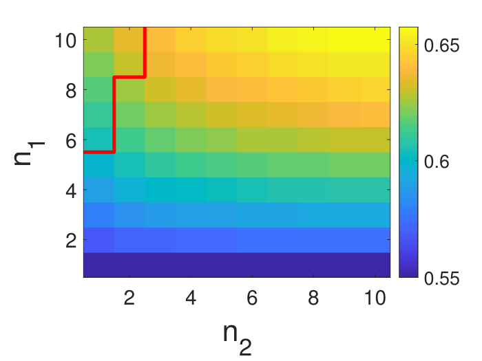
which, as we detail in SUPMAT, provides an upper bound to the average fidelity attainable when resorting on MP strategies when having copies of A and arbitrary copies of . The curves show that for the low value we are considering here, the MP procedures are ineffective even with respect to the trivial DN strategy. on the contrary is strictly larger than the DN score. Also it is very close to , showing that for , the possibility of having just a single copy of the perturbing state provides us almost all the benefit one could obtain by having a classical knowledge of the latter. For larger values of and analytical treatment becomes cumbersome and we resort to numerical analysis using Mathematica Mathematica to compute the parameters of the problem and CVX, a package for specifying and solving convex programs MATLAB; CVX1; CVX2 in Matlab, to calculate the maximum fidelity values. Results are reported in Fig. 2 for and and .
 |
 |
V Conclusions
The gap between and the DN strategy (which is optimal in the scenario and independent from the explicit value of ) shows that even a small redundancies on the input A, can be beneficial. On the contrary, the very small distance between and clarifies that gathering more information on the mixing term (the noise of the model) does not help too much. As can be seen from Fig. 2 for larger and one can instead see a noise-dependent separation line between two regions, one where it is indeed advantageous to increase instead of and the other where the opposite holds.
The symmetry of the problem allowed us to reduce exponentially the number of variables involved in the optimisation. The same analysis should be relevant also in a broader perspective for general noise models.
VI Acknowledgments
The first two authors contributed equally to this work.
References
- (1) R. F. Werner, Springer Tracts in Modern Physics, Eprint arXive: arXiv:quant-ph/0101061.
- (2) W. K. Wootters and W. H. Zurek, Nature 299, 802 (1982).
- (3) D. Dieks, Phys. Lett. A 92, 271 (1982).
- (4) M. A. Nielsen and I. L. Chuang, Phys. Rev. Lett. 79, 321 (1997).
- (5) A. Kumar Pati and S. L. Braunstein, Nature 404, 164 (2000).
- (6) M. Piani, P. Horodecki, and R. Horodecki, Phys. Rev. Lett. 100, 090502 (2008).
- (7) U. Alvarez-Rodriguez, M. Sanz, L. Lamata, and E. Solano, Sci. Rep. 5, 11983 (2015).
- (8) M. Oszmaniec, A. Grudka, M. Horodecki, and A. Wojcik, Phys. Rev. Lett. 116, 110403 (2016).
- (9) V. Scarani, S. Iblisdir, N. Gisin, and A. Acín, Rev. Mod. Phys. 77 1225 (2005).
- (10) M. Doosti, F. Kianvash, and V. Karimipour, Phys. Rev. A 96, 052318 (2017).
- (11) S. Dogra, G. Thomas, S. Ghosh, and D. Suter, Phys. Rev. A 97, 052330 (2018).
- (12) P. Hayden, S. Nezami, S. Popescu, G. Salton, arXiv:1709.04471 [quant-ph].
- (13) S. D. Bartlett, T. Rudolph, and R. W. Spekkens, Rev. Mod. Phys. 79, 555 (2007).
- (14) G. Gour, and R. W. Spekkens, New J. Phys. 10, 033023 (2008).
- (15) J. C. Boileau, L. Sheridan, M. Laforest, and S. D. Bartlett, Journal of Mathematical Physics 49, 032105 (2008).
- (16) P. Wittek, Quantum machine learning: what quantum computing means to data mining (Academic Press, 2014).
- (17) V. Dunjko and H. J. Briegel, Eprint arXiv:1709.02779.
- (18) J. Biamonte, P. Wittek, N. Pancotti, P. Rebentrost, N. Wiebe and S. Lloyd, Nature 549, 195-202 (2017).
- (19) J. Fiurášek, New J. of Phys. 8, 192 (2006).
- (20) G. Chiribella and G. M. D’Ariano, Phys. Rev. Lett. 97, 250503, (2006).
- (21) D. Bruss, A. Ekert, and C. Macchiavello, Phys. Rev. Lett. 81, 2598 (1998).
- (22) A. Chefles and S. M. Barnett, Journal of Physics A: Mathematical and General 31(50), 10097, (1998).
- (23) A. S. Holevo, Quantum Systems, Channels, Information:A Mathematical Introduction (De Gruyter 2012).
- (24) M. A. Nielsen and I. L. Chuang, Quantum Computation and Quantum Information (Cambridge: Cambridge University Press, 2010).
- (25) V. Scarani et al., Phys. Rev. Lett. 88, 097905 (2002)
- (26) J. I. Cirac, A. K. Ekert, and C. Macchiavello, Phys. Rev. Lett. 82, 4344 (1999).
- (27) C. King, IEEE Trans. Inf. Theory 49, 221-229, (2003).
- (28) T. D. Ladd , F. Jelezko, R. Laflamme, Y. Nakamura, C. Monroe, and J. L. O’Brien, Nature 464, 45 (2010).
- (29) N. Gisin and R. Thew, Nat. Phot. 1, 165 (2007).
- (30) M. Ippoliti, L. Mazza, M. Rizzi, and V. Giovannetti, Phys. Rev. A 91, 042322 (2015).
- (31) V. Buźek and M. Hillery, Phys. Rev. A 54, 1844 (1996).
- (32) R. F. Werner, Phys. Rev. A 58, 1827 (1998).
- (33) N. Gisin and S. Massar, Phys. Rev. Lett. 79, 2153 (1997).
- (34) D. Bruss, A. Ekert, and C. Macchiavello, Phys. Rev. Lett. 81, 2598 (1998).
- (35) V. Scarani, S. Iblisdir, N. Gisin, and A. Acín, Rev. Mod. Phys. 77, 1225 (2005).
- (36) A. S. Holevo, Eprint arXiv:quant-ph/0212025.
- (37) S. Massar and S. Popescu, Phys. Rev. Lett. 74, 1259 (1995)
- (38) W. Fulton and J. Harris, Representation theory. A first course. Graduate Texts in Mathematics, Readings in Mathematics. 129. New York: Springer-Verlag (1991).
- (39) L. Vandenberghe, and S. Boyd, SIAM Review Vol. 38, No. 1 (Mar., 1996), pp. 49-95
- (40) Wolfram Research, Inc., Mathematica, Version 11.3, Champaign, IL (2018).
- (41) MATLAB and Statistics Toolbox Release 2018b, The MathWorks, Inc., Natick, Massachusetts, United States.
- (42) M. Grant and S. Boyd. CVX: Matlab software for disciplined convex programming, version 2.1. http://cvxr.com/cvx, December 2018.
- (43) M. Grant and S. Boyd. Graph implementations for nonsmooth convex programs, Recent Advances in Learning and Control (a tribute to M. Vidyasagar), V. Blondel, S. Boyd, and H. Kimura, editors, pages 95-110, Lecture Notes in Control and Information Sciences, Springer, 2008. http://stanford.edu/~boyd/graph_dcp.html.
- (44) A. W. Knapp, Lie Groups Beyond an Introduction Birkhauser-Verlag, Basel, (1996).
- (45) Details of the calculations are available in the Supplemental Material at [URL will be inserted by publisher], where Knapp is cited.
VII Appendix
Supplemental material is organised as following. First, we provide explicit derivation of the decomposition (16) of the main text. Then using (16) we derive the fidelity (20) of the main text. Third, we present an explicit derivation of Eq. (23) of the main text. Then we analyze the application of the decomposition (16) of the main text to the case where , and in the following section we do the same for the case . Analytical optimisation is also done for the case . Then, we present the derivation of an upper bound for the average fidelity of the UQS realised via measurement and prepare strategies. Finally, we apply the method of Cirac et al. CIRAC for case and arbitrary .
VII.1 Covariant Channel Characterisation
Here the calculations to derive the characterisation for covariant are presented. Introducing a Kraus decomposition for in Eq.(14) of the main text we get
| (26) |
with the associated Kraus operators. Accordingly we can express the matrix element (16)
| (27) |
where
| (28) |
We can write the multiplication of two Wigner matrices in the following form
| (29) | |||||
where are the Clebsch-Gordan coefficients. Exploiting this we can hence rewrite Eq. (27) in the following form
| (30) | |||||
Remembering that following identity of Wigner matrices (Peter-Weyl theorem, see Knapp)
| (31) |
the integral in (30) can hence be simplified to
| (32) | |||||
Introducing then the variable , we can rewrite the above identity as
| (33) | |||||
which, defining the row vectors of components
| (34) |
and their associated scalar products
| (35) |
allows us to finally express Eq. (33) as in Eq. (16) of the main text
| (36) |
VII.2 Fidelity calculation for arbitrary and numerical optimisation
Using Eq. (13) of the main text the average fidelity can be expressed as
| (37) |
Knowing that is invariant under any permutation on the first qubits, we can write
| (38) |
where is a permutation on the first qubits, and runs over all the elements of the symmetric group , and is the number of elements of symmetric group. Then we can write
| (39) |
where . Defining , we carry on the calculation
| (40) | |||||
Note that here we do not need to sum over any multiplicity index for the states and , because is supported on the completely symmetric subspace of qubits, therefore it is also supported on the tensor product of the completely symmetric subspaces of and qubits, which have multiplicity 1. Writing the first qubits in the total angular momentum basis we get
| (41) | |||||
here the multiplicity index indicates that we first wrote the qubits in the total angular momentum basis then we summed it up with . Schur’s lemma implies
| (42) |
where is the index for the multiplicity of and runs over all the possible values for a certain , and . Using Eq. (42) in Eq. (39) we get
| (43) | |||||
Using the Eq. (16) of the main text we get
| (44) | |||||
The dependence of the coefficients of on the multiplicity index is only through . So, we can define
| (45) | |||||
and write the fidelity as
| (46) |
Because is symmetric on the first qubits, we can always choose to be symmetric on the first qubits, therefore
| (47) |
Using (42) we derive
| (48) |
therefore
| (49) |
so defining , then we get
| (50) |
Now, the number of parameters i.e. , scale polynomially with and because the multiplicity index is fixed to be and the number of different is . Without using the characterisation of covariant channels and writing in the proper form, the number of parameters grows exponentially in and . This exponential reduction of parameters makes the numerical optimisation feasible. In fact, this optimisation problem is exactly a semidefinite programming optimisation. To show this we first briefly review the semidefinite programming and then we define the parameters in the program.
A general semidefinite program can be defined as any mathematical program of the form SDP
| (51) | |||
where is the space of all real matrices. and are real matrices, and are real numbers and means that is semidefinite.
In our problem, are the matrix elements of which are all real since is the combination of the Clebsch-Gordan coefficients. Our constraints are equality constraints, each of which can be obtained from two inequalities. The matrix elements of are , and the elements of and can be read from the coefficients in Eq. (23) of the main text.
To prove that our problem is a semidifinite program we should show that is positive-semidefinite. is positive-semidefinite if and only if there exists a set of vectors like such that . In the definition of in Eq. (35), we have
| (52) |
and using Eq. (49) we get
| (53) |
So, and our problem is a semidefinite program.
Note that in our maximisation problem the parameters in general can be complex numbers. However, the matrix elements of are the contraction of Clebsch-Gordan coefficients which are all real, therefore without loss of generality we can assume that are real.
VII.3 Derivation of Eq. (17)
Here we give explicit derivation of the constraint (15) of the main text. The starting point to observe that by explicit substitution of Eq. (13) into Eq. (14) of the main text we get
| (54) |
Using then the following symmetry property of Clebsch-Gordan coefficients
| (55) |
we can observe that
| (56) |
where is the projector on the the eigenspace. It follows hence that (54) is automatically fulfilled for , while for instead it gives (17) of the main text
| (57) |
Using the definition of and summing the equations (57) we get
| (58) |
VII.4 Application of the formalism to the case
For , Eq. (13) of the main text explicitly yields
| (59) |
Notice that the term is invariant under rotations hence it gets mapped by into a multiple of the identity operator: specifically noticing that we have which implies . On the contrary the first contribution to admits the following decomposition
| (60) |
where without loss of generality we identified with the vector , and where in the r.h.s. appear states of the total angular momentum basis of two spin (no multiplicity being present). Using Eq. (16) of the main text and the table of Clebsch-Gordan coefficients we can then write
| (61) | |||||
where we dropped the index since here is no multiplicity in total angular momentum basis of two qubits. Similarly the constraints (23) of the main text becomes
| (62) |
Exploiting this we observe that fidelity of for a generic map must fulfil the constraint
| (63) | |||||
the first inequality being obtained by forcing and to be collinear, while the second following directly from (62). By comparing this with the lower bound discussed in the main text for the qubit case (i.e. ) this allows us to recover the identity (10) of the main text, i.e.
| (64) |
the bound being achived by employing the DN strategy.
VII.5 Details of the Calculation for
Here we present detailed calculation to derive Eq. (18) of the main text. Using the Eq. (44) we can write the fidelity as
| (65) | |||||
using the definition of and the definition of in Eq. (35) we can write
| (66) | |||||
with constraints:
| (67) |
where . Using the constraints we eliminate , Eq. (66) becomes
| (68) |
The coefficients of are positive everywhere, so to maximise the fidelity we put their maximum values , obtaining
| (69) |
This last expression has to be maximise with respect to considering that, according to the constraint (67) such variable has to belong to the interval . For the case we take the derivative and put it equal to zero obtaining
| (70) |
which belongs to the allowed interval only when . Accordingly for these values of we can use Eq. (70) obtaining
| (71) |
For the case (which incidentally also includes ), instead the maximum for (68) is always maximised for the maximum allowed value of , i.e. yielding
| (72) |
which together with (71) gives us (18) of the main text.
VII.6 Case ,
As we argued in the text,
| (73) |
This equality is consistent since does not depend on by virtue of the invariance property of the Haar measure, and therefore one can set without loss of generality. In this case the optimal is not covariant, since it depends on , but we can still find the maximum fidelity through the standard Kraus representation of . For , there is no need to distinguish between equivalent representations and the matrix elements of a set of Kraus operators for , , satisfy
| (74) | ||||
| (75) |
The integral in (73) can be written as
| (76) |
where
| (77) |
After performing the integrations the result is
| (78) |
Using the constraints (23) and the positivity and magnitude of the coefficients most of the optimal parameter choices can be found:
Moreover, using the Cauchy-Schwartz inequality
| (79) |
one is left with the maximisation of a function of the variable :
| (80) |
The solution and the maximal value of the fidelity can be analytically determined, but they are quite cumbersome and we do not report them: instead we present the numerical plot in Fig. 2 of the main text.
VII.7 Upper Bound on Measurement and Prepare Protocols
We have already observed that in the limit of large and , MP protocols allows for optimal average fidelity. But what happens for finite number of copies? To answer this question we introduce an upper bound on the average fidelity attainable with MP protocols. Indeed, invoking once more the fact that for characterizing optimal performances one can restrict the analysis to transformations which are symmetric under the permutation of the first qubits. Using Eq. (39), the associated fidelity can be written as
| (81) |
where now is the optimal MP channel. Then, we can get the following upper bound by using an optimal MP for each independent part of the whole state
| (82) | |||||
where is the optimal MP choice for . Using the known result for tomography of pure states Massar Pure we can then derive the following inequality
| (83) |
where is the average fidelity in the optimal tomography of copies of a pure state. Notice that the right-hand-side quantity does not depend explicitly on , and that for reduces to the function (19) of the main text which we reported in Fig. 1.
VII.8 Performance of the Cirac, Ekert, Macchiavello (CEM) protocol as a subtracting machine
Here we show that a direct application of the method of Ref. CIRAC to solve our problem for and arbitrary leads to the same average fidelity as the DN strategy, being hence sub-optimal for our purposes.
The method presented in Ref. CIRAC does not assume the possibility of operating on the noise signal, therefore the average fidelity one can achieve in this case does not depend on . For case , it consists of two steps first performing an orthogonal measurement on the system that discriminate the completely symmetric from the antisymmetric subspace of two qubits, and then tracing out on of the qubits. Adopting this procedure from Eq. (4) of the main text we get
| (84) | |||||
Taking the integral on and using the fact that the method CIRAC is also covariant we can carry on the calculation
| (85) | |||||
where in the last inequality we use the fact that, as anticipated, consists in performing the measurements on the symmetric and antisymmetric subspace. We notice hence that exactly coincides with the fidelity one would get by simply adopting the DN strategy, i.e. which is clearly not optimal in our case.