Evolution of Cosmological Horizons of Wormhole Cosmology

Sung-Won Kim email:sungwon@ewha.ac.kr Affiliation: Department of Science Education, Ewha Womans University, Seoul 03760, Korea

today

Abstract

Recently we solved the Einstein’s field equations to obtain the exact solution of the cosmological model with the Morris-Thorne type wormhole. We found the apparent horizons and analyzed their geometric natures, including the causal structures. We also derived the Hawking temperature near the apparent cosmological horizon. In this paper, we investigate the dynamic properties of the apparent horizons under the matter-dominated universe and lambda-dominated universe. As a more realistic universe, we also adopt the $\Lambda$ CDM universe which contains both the matter and lambda. The past light cone and the particle horizon is examined for what happens in the case of the model with wormhole. Since the spatial coordinates of the spacetime with the wormhole are limited outside the throat, the past light cone can be operated by removing the smaller-than-wormhole region. The past light cones without wormhole begin start earlier than the past light cones with wormhole in conformal time-proper distance coordinates. The light cone consists of two parts: the information from our universe and the information from other universe or far distant region through the wormhole. Therefore, the particle horizon distance determined from the observer’s past light cone can not be defined in a unique way.

I introduction

Recently kim2018 we derived the exact solution of the cosmological model with a wormhole by using the method similar to that of McVittie MV who had obtained the black hole solution in the flat Friedmann-Lemaitre-Robertson-Walker (FLRW) universe. Even though there are several example models for wormhole cosmology 3-BF, they did not guarantee the Einstein equation.

It is well known that there are two prototypes of wormhole: the Morris-Thorne wormhole MT and the Visser wormhole visser. Thus, the wormhole cosmological model is based on these two models. Kim 3, Hochberg hochberg, Li Li, Bochiccio and Faraoni BF dealt with the Visser type thin-shell wormhole to construct a cosmological model with a wormhole. Usually, we prepare two copies of the appropriate model, cut off the central parts of the copies, and paste the remaining two pieces to the cut edge. This junction plays the role of wormhole throat connecting two universe models. As an example of minimizing the use of exotic matter at the junction, we can consider the delta function distribution of the matter. It is an easy way to do it by hands, but it is an unnatural way to create a wormhole.

Another way to construct a cosmological model with a wormhole is to start with a Morris-Thorne type wormhole. We combine the wormhole and the cosmological background by hand with plausibility. Later we can find the satisfactory matter conditions from the Einstein’s equation, but this is not a natural way either. Roman roman, Kim kim, González-Díaz Gon, and Mirza et al. MED, used MT wormhole to construct a cosmological models with a wormhole.

The solution we got kim2018 was unique in the sense of satisfying Einstein’s equation with Morris-Thorne type wormhole starting from the generic isotropic spacetime. We also got two apparent horizons by transforming to the Schwarzschild-like coordinates: one is the apparent cosmological horizon and the other one is the wormhole throat. It is important to know how the cosmic matter affects the spacetime of the wormhole cosmology and its horizons, because we can get the role of wormhole in the universe from the information. The dynamic nature of the spacetime and cosmological horizons is as important as the causal nature in analyzing the wormhole cosmological model and understanding the physics of the universe.

In this paper, we considered their dynamic nature of the apparent horizons under the background cosmological models. The background models considered here are the matter- and/or lambda-dominated universe. Recent observations planck reveal that the spacetime is nearly flat ( $\Omega_{k}\simeq 0$ ) and the most probable model is $\Lambda$ CDM universe. In this case radiation is usually neglected, so the model with the matter and lambda is simpler.

We need to know how the wormhole affects on the geometry of the universe. Therefore, in each universe, the creation and dynamics of the apparent horizons, past light cone, and particle horizon distance are investigated and the characteristics of the model with the wormhole are found. The apparent cosmological horizon has the meaning of the modified Hubble horizon, because it approaches the Hubble horizon in the absence of a wormhole. The role of the Hubble horizon in the universe is the boundary between particle at a speed smaller than the speed of light $c$ and the particle at a speed higher than $c$ relative to the observer of a given time. Thus we can say that the apparent cosmological horizon constitute a sphere containing all the astronomical systems, in this spacetime, at the time of observation receding from the observer slower than the light. The speeds of the horizons are also discussed because they are useful for viewing their dynamics. The apparent horizons’ speeds are compared with the Hubble surface speed and the wormhole speed.

Since the particle horizon is defined as the maximum distance that particles could have traveled to the current observer, this consideration gives us the information of the spacetime’s causal structure as well as the light cone. The particle horizon distance is decided by the observer’s past light cone Harrison. An observer’s particle horizon divides all world lines into two classes at the moment of observation: those that intersect the observer’s past light cones, and those that lie outside the reach of the observer’s light cone. We should know how past light cone and particle horizon distance are changed for spacetime of the universe with a wormhole. We can also discussed on the issue of horizon problem and introduction of the inflation in the early universe in big bang scenario.

In Sec 2, we briefly summary the solution of the wormhole cosmology and the structure of the apparent horizons. In Sec 3, we investigate the time evolution of the Hubble horizon, particle horizon, light cone for the model with a wormhole depending on the matters in the universe. Summary and discussion are in final section.

II Exact solution and apparent horizons

The Morris-Thorne type wormhole (MT-wormhole) is given by MT

ds^{2}=-e^{2\Phi}dt^{2}+\frac{1}{1-b(r)/r}dr^{2}+r^{2}d\Omega^{2},

(1)

where $\Phi(r)$ is red-shift function and $b(r)$ is the shape function. The geometric unit, that is, $G=c=\hbar=1$ is used here. The radius $r$ is in the range of $b<r<\infty$ . Two functions $\Phi(r)$ and $b(r)$ are restricted by ‘flare-out condition’ to maintain the shape of the wormhole.

The isotropic form of the static wormhole, to see it under FLRW universe, is

ds^{2}=-d\tilde{t}^{2}+\left(1+\frac{b_{0}^{2}}{4\tilde{r}^{2}}\right)^{2}(d\tilde{r}^{2}+\tilde{r}^{2}d\Omega^{2})

(2)

for the ultra-static case ( $\Phi^{\prime}=0,~~b(r)=b_{0}^{2}/r$ ). Here coordinates with tilde mean the transformed coordinate to the isotropic wormhole. The radial coordinate is $\tilde{r}>b_{0}/2$ in isotropic form (2), while $r>b_{0}$ in spherically symmetric form (1). However, we will omit the tilde over coordinates by convenience from now on, if only there are no confusions.

The FLRW spacetime in isotropic form is given by MV

ds^{2}=-dt^{2}+\frac{a^{2}(t)}{(1+kr^{2})^{2}}(dr^{2}+r^{2}d\Omega^{2}).

(3)

Here $a(t)$ is the scale factor and $k=1/4{\cal R}^{2}$ , where ${\cal R}$ is the curvature, and $k$ goes zero in case of flat FLRW spacetime. We start from the general isotropic metric element to see the unified wormhole in FLRW cosmological model as

ds^{2}=-e^{\zeta(r,t)}dt^{2}+e^{\nu(r,t)}(dr^{2}+r^{2}d\Omega^{2}).

(4)

Einstein’s equation is given by

G_{\alpha\beta}=\kappa T_{\alpha\beta},

where $\kappa=8\pi$ . The non-zero components of Einstein tensor ${G^{\mu}}_{\nu}$ are

$\displaystyle{G^{0}}_{0}$	$\displaystyle=$	$\displaystyle\frac{1}{4r}\{[(8\nu^{\prime}+4\nu^{\prime\prime}r+\nu^{\prime 2}r)e^{-\nu+\zeta}-3\dot{\nu}^{2}r]e^{-\zeta}\},$	(5)
$\displaystyle{G^{0}}_{1}$	$\displaystyle=$	$\displaystyle\frac{1}{2}(2\dot{\nu}^{\prime}-\dot{\nu}\zeta^{\prime})e^{-\zeta},$	(6)
$\displaystyle{G^{1}}_{1}$	$\displaystyle=$	$\displaystyle\frac{1}{2r}\{[r(-2\ddot{\nu}+(-\frac{3}{2}\dot{\nu}+\dot{\zeta})\dot{\nu})e^{-\zeta+\nu}+2\nu^{\prime}+2\zeta^{\prime}+\zeta^{\prime}\nu^{\prime}r+\frac{1}{2}r\nu^{\prime 2}]e^{-\nu}\},$	(7)
$\displaystyle{G^{1}}_{0}$	$\displaystyle=$	$\displaystyle\frac{1}{2}(-2\dot{\nu}^{\prime}+\dot{\nu}\zeta^{\prime})e^{-\nu},$	(8)
$\displaystyle{G^{2}}_{2}$	$\displaystyle=$	$\displaystyle{G^{3}}_{3}=\frac{1}{4r}\{[2\zeta^{\prime}+2\nu^{\prime}+2\nu^{\prime\prime}r+2\zeta^{\prime\prime}r+\zeta^{\prime 2}r]e^{-\nu}+2r(-2\ddot{\nu}-\frac{3}{2}\dot{\nu}^{2}+\dot{\zeta}\dot{\nu})e^{-\zeta+\nu}\}.$	(9)

Here dot denotes the derivation with respect to $t$ and prime denotes the derivative with respect to $r$ .

By solving the Einstein’s equation, the exact cosmological wormhole solution is given by kim2018

ds^{2}=-dt^{2}+\frac{a^{2}(t)}{(kr^{2}+1)^{2}}\left(1+\frac{b_{0}^{2}}{4r^{2}}\right)^{2}(dr^{2}+r^{2}d\Omega^{2}).

(10)

It is assumed that the radial accretion is not allowed in this model like the Mc Vittie solution MV. Here $a(t)$ is the scale factor and $k$ is the curvature parameter of FLRW cosmology. The model shows that the cosmic part and the wormhole part are multiplied, so that the spatial and the temporal parts are separated. The resultant spacetime is natural, since the ansatz for the matter distribution (cosmic matter and wormhole matter) is separable during finding the solution, such as

$\displaystyle a^{2}(t)\rho(r,t)$	$\displaystyle=$	$\displaystyle a^{2}(t)\rho_{c}(t)+\rho_{w}(r),$	(11)
$\displaystyle a^{2}(t)p_{1}(r,t)$	$\displaystyle=$	$\displaystyle a^{2}(t)p_{1c}(t)+p_{1w}(r),$	(12)
$\displaystyle a^{2}(t)p_{2}(r,t)$	$\displaystyle=$	$\displaystyle a^{2}(t)p_{2c}(t)+p_{2w}(r),$	(13)
$\displaystyle a^{2}(t)p_{3}(r,t)$	$\displaystyle=$	$\displaystyle a^{2}(t)p_{3c}(t)+p_{3w}(r),$	(14)

which is the method like the separation of variables in partial differential equation of many physical problems. This ansatz were already used in the previous wormhole cosmological model kim.

When we change (10) into the Schwarzschild-like form in new coordinate $R$ , the spacetime will be

ds^{2}=-\left(1-\frac{R^{2}H^{2}}{r^{2}J^{2}}\right)dt^{2}+\frac{1}{r^{2}J^{2}}dR^{2}-\frac{2HR}{r^{2}J^{2}}dtdR+R^{2}d\Omega^{2},

(15)

where

R\equiv a(t)\left(\frac{(1+b_{0}^{2}/4r^{2})}{(1+kr^{2})}\right)r=a(t)A(r)\quad\mbox{and}\quad J\equiv\frac{A^{\prime}}{A}.

(16)

To remove $dtdR$ -term, by defining

dT=\frac{1}{F}(dt+\beta dR),

(17)

the spacetime can be

ds^{2}=-\frac{H^{2}({R_{+}}^{2}-R^{2})(R^{2}-{R_{-}}^{2})}{R^{2}-a^{2}b_{0}^{2}}F^{2}dT^{2}+\frac{1}{r^{2}J^{2}}\frac{R^{2}-a^{2}b_{0}^{2}}{H^{2}({R_{+}}^{2}-R^{2})(R^{2}-{R_{-}}^{2})}dR^{2}+R^{2}d\Omega^{2}.

(18)

Here $R_{\pm}$ are the location of the apparent horizons

R_{\pm}=\frac{1}{\sqrt{2H^{2}}}[1\pm\sqrt{1-(2b(t)H)^{2}}]^{1/2}<R_{\rm H}\equiv\frac{1}{H},

(19)

where $b(t)\equiv a(t)b_{0}$ is the extended wormhole with a scale factor, as seen in the isotropic metric of the wormhole. This is the previous time dependencies of the cosmological wormholes roman; kim that expand along the scale factor. The modified wormhole in their works also satisfied the flare-out condition and their roles in the spacetime. Here, $R_{+}$ means the apparent cosmological horizon, and $R_{-}$ is the minimum size of dynamic wormhole throat in this spacetime. The condition of $(2b(t)H)^{2}<1$ is required for these two horizons $R_{\pm}$ to be real values. This condition decide the existence of the two horizons and the coincidence time of them.

For the FLRW universe without wormholes, the Hubble surface defined by $R_{\rm H}=1/H$ that is the boundary between the subluminal inner sphere and the superluminal outer sphere. The Hubble horizon $R_{\rm H}$ is always outside the apparent horizons. If the wormhole vanishes in the universe, $b_{0}=0$ , $R_{+}$ approaches the Hubble horizon and $R_{-}$ disappears. Thus, the apparent cosmological horizon acts as the Hubble horizon in the universe with wormhole. In the region smaller than the sphere of radius $R_{+}$ of this spacetime, any particle travels slower than the light. At the limit of $a(t)$ =const ( $H=0$ ), $R_{-}$ approaches to $b_{0}$ . That is, when the cosmological background is removed from this model, the spacetime becomes the MT wormhole.

III Time evolution of the horizon

III.1 Power law distribution

Now we apply the issues to the various distributions for cosmic part of the universe. Above all, we have to check the Friedmann equation to see if there are changes in the equation by a wormhole in this spacetime. The Friedmann equation for the wormhole cosmological model is

H^{2}\equiv\left(\frac{\dot{a}}{a}\right)^{2}=\frac{8\pi\rho_{c}}{3},

(20)

which is the same as for a model without a wormhole because time-dependence of $\rho_{c}$ and time-independence of $\rho_{w}$ are completely separated as wee see in (14). With energy conservation law $\dot{\rho}_{c}+3H(\rho_{c}+P_{c})=0$ and the equation of state $P_{c}=\omega\rho_{c}$ , the scale factor $a$ and Hubble parameter will be

a=\left(\frac{t}{t_{0}}\right)^{2/(3+3\omega)}\equiv\left(\frac{t}{t_{0}}\right)^{q}\quad\mbox{and}\quad H\equiv\frac{\dot{a}}{a}=\frac{q}{t},

(21)

when $a(t)$ follows the power law and $\omega$ is the parameter of the equation of state. The present time, the age of our universe $t_{0}$ is

t_{0}=\frac{1}{1+\omega}\left(\frac{1}{6\pi\rho_{c}}\right)^{1/2}\quad(\omega\neq-1)

(22)

and $a_{0}\equiv a(t_{0})=1$ , is the present scale factor. The Hubble surface recede at the radial velocity

\frac{dR_{\rm H}}{dt}=\frac{1}{q}=1+\xi,

(23)

where $\xi=-\ddot{a}a/\dot{a}^{2}$ the deceleration parameter and the dot means the differentiation with respect to time $t$ .

Now we discuss the time evolutions of apparent horizons according to the cosmic matter distributions of the background universe. Since the background universe model is FLRW, we will consider the matter-universe models with and/or without lambda. Due to the time-dependence $a(t)$ and $H(t)$ , the apparent horizons do evolve and expand or collapse. The apparent cosmological horizons $R_{\pm}$ with time-dependencies (21) for the power law, are represented in terms of time $t$ as

R_{\pm}(t)=\frac{t}{\sqrt{2}|q|}[1\pm\sqrt{1-(2qb_{r})^{2}(t/t_{0})^{2(q-1)}}]^{1/2},

(24)

where $b_{r}\equiv b_{0}/t_{0}$ is the relative wormhole size. The time when two horizons coincide is

t_{\rm c}=(2qb_{r})^{1/(1-q)}t_{0}

(25)

and the size of the resultant horizons is

R_{\rm c}=\frac{(2qb_{r})^{1/(1-q)}}{\sqrt{2q^{2}}}t_{0}=\frac{t_{\rm c}}{\sqrt{2q^{2}}}

(26)

at that time. The wormhole has the size restricted as

b_{r}<\frac{1}{2q}\left(\frac{t}{t_{0}}\right)^{(1-q)}

(27)

for the existence of $R_{\pm}$ in (24).

To see the time evolutions of the horizon, the time derivatives of the horizons are

	$\displaystyle\frac{d}{dt}R_{\pm}$	$\displaystyle=$	$\displaystyle\frac{1}{\sqrt{2}\|q\|}\left\{[1\pm\sqrt{1-Bt^{2(q-1)}}]^{1/2}\right.$		(28)
			$\displaystyle\left.\mp\frac{1}{2}\frac{Bt^{2(q-1)}(q-1)}{[1\pm\sqrt{1-Bt^{2(q-1)}}]^{1/2}\sqrt{1-Bt^{2(q-1)}}}\right\},$		(28)

where $B=(2qb_{0})^{2}(t_{0})^{-2(q-1)}$ . The $R_{-}$ has the minimum value at

t_{\rm min}=[\sqrt{q}(1+q)b_{r}]^{1/(1-q)}t_{0}

(29)

just after the coincidence time $t_{\rm c}$ and increases after $t_{\rm min}$ with (28). The ratio of $t_{\rm min}$ to $t_{\rm c}$ is

\frac{t_{\rm min}}{t_{\rm c}}=\left(\frac{(1+q)^{2}}{4q}\right)^{1/2(1-q)}>1,\quad\mbox{for}\quad 0<q<1

(30)

and is depends only on $q$ and does not depend on $b_{r}$ or $t_{0}$ . This ratio is larger as the value of $q$ is smaller. The minimum value of $R_{-}$ at $t=t_{\rm min}$ is

R_{-}^{(\rm min)}=\frac{1}{\sqrt{q(1+q)}}\frac{t_{\rm min}}{t_{0}}.

(31)

The reason of the existence of minimum value of $R_{-}$ is that $R_{-}$ is given as the product of the linearly increasing part and the decreasing part (for $q<1$ ) in time as shown in (24). Therefore, $\dot{R}_{-}<0$ before $t_{\rm min}$ and $\dot{R}_{-}>0$ after $t_{\rm min}$ . It can be said that the wormhole is initially contracted and expands with the very high expansion of the universe. The expansion of the universe close to the coincidence time prevails the expansion of the wormhole, so the wormhole shrinks before $t_{\rm min}$ .

At very early times when the horizons was created, the speeds of the apparent horizons diverge near $t_{\rm c}$ , such as

\lim_{t\rightarrow t_{\rm c}}\frac{dR_{\pm}}{dt}=\pm\infty.

(32)

As time goes on, $dR_{+}/dt$ decreases and $dR_{-}/dt$ increases from negative to positive, so $R_{-}$ has the minimum value. In the distant future, the speeds of the horizons are given as

	$\displaystyle\lim_{t\rightarrow\infty}\frac{dR_{+}}{dt}$	$\displaystyle=$	$\displaystyle\frac{1}{\|q\|},$		(33)
	$\displaystyle\lim_{t\rightarrow\infty}\frac{dR_{-}}{dt}$	$\displaystyle=$	$\displaystyle b_{0}q\left(\frac{t}{t_{0}}\right)^{(q-1)}=b_{0}\dot{a},$		(34)

for positive $q$ . The speed of ${R}_{+}$ approaches the speed of Hubble surface and $R_{-}$ will eventually stop when $q<1$ in flat universe.

III.2 Matter-dominated universe

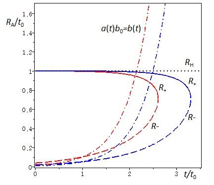
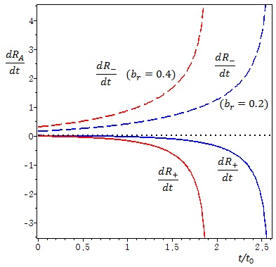
For matter-dominated universe $\omega=0$ , $q=2/3$ , $a(t)=(t/t_{0})^{2/3},$ and $H(t)=\frac{2}{3t}$ . The time-dependencies of apparent horizons and their speeds are depicted in Fig. 1. The equation (8) shows that two horizons do not appear before $t_{\rm c}^{\rm(m)}$ , where $t_{\rm c}^{\rm(m)}=(4b_{r}/3)^{3}t_{0}$ is the time when the two horizons are generated and separated simultaneously in the matter-dominated universe. Prior to $t_{\rm c}^{\rm(m)}$ , the wormhole matters are highly localized at very tiny region and cannot generate $R_{\pm}$ , because $H$ is very large as can be seen in the square root of the equation (24). Then, as the speed of the scale factor decreases, the horizons $R_{\pm}$ appear and expand with the scale factor. The size of the horizons at the coincidence time is just

R_{\rm c}^{\rm(m)}=\frac{16}{9}\sqrt{2}b_{r}^{3}t_{0}.

(35)

For larger the wormhole, the later the coincidence time. When the more matter is concentrated to construct the wormhole, the generation time of wormhole and apparent horizon will be delayed. When universe expands, the two horizons also expand, but the expansion rate of $R_{+}$ is higher than that of $R_{-}$ , so they can never meet again. At a late time, $R_{+}$ approaches $R_{\rm H}$ and $R_{-}$ approaches $b(t)=b_{0}(t/t_{0})^{2/3}$ . Just after the coincidence time, the size of the wormhole, $R_{-}$ , decreases before the time $t_{\rm min}^{(\rm m)}=(\sqrt{50/27}b_{r})^{3}t_{0}$ and increases after that time. The ratio of $t_{\rm min}^{\rm(m)}$ to $t_{\rm c}^{\rm(m)}$ is

\frac{t_{\rm min}^{\rm(m)}}{t_{\rm c}^{\rm(m)}}=\left(1+\frac{1}{24}\right)^{3/2}.

(36)

The minimum size of the wormhole at that time is

R_{-}^{(\rm min)}=\frac{50}{81}\sqrt{15}b_{r}^{3}.

(37)

If the wormhole size $b_{0}$ is smaller, the time of wormhole minimum size is closer to $t=0$ , since $t_{\rm c}$ is proportional to $b_{r}^{3}$ .

For the speed of horizon as we see Fig. 1(b), the speed of $R_{+}$ is very large near the coincidence time and rapidly approach the speed of $R_{\rm H}$ . At the very early time, $dR_{+}/dt>dR_{\rm H}/dt$ , and later the inequality sign reverses. Finally $dR_{+}/dt$ approaches $dR_{\rm H}/dt$ . The speed of $R_{-}$ approaches to $-\infty$ near coincidence time and will change from negative to positive at $t=t_{\rm min}^{(\rm m)}$ . Finally $dR_{-}/dt$ approaches $b_{0}(t_{0}/t)^{(1/3)}$ and in the far future $R_{-}$ will stop expanding like the scale factor of zero curvature cosmological model.

III.3 Lambda-dominated universe

In the lambda-dominated universe, the attributes of $a,\dot{a},H$ , and $\dot{H}$ are quite different from those of power-law expansion of the scale factor. In this universe, $a=e^{H_{0}(t-t_{0})}$ instead of the power law and $H=H_{0}={\rm const}$ . At very early times, they are completely separate as shown in Fig 2. Two horizons exist for $t<t^{\rm(\Lambda)}_{\rm c}=t_{0}-\ln(2H_{0}t_{0}b_{r})/H_{0}$ and two horizons meet at $t^{\rm(\Lambda)}_{\rm c}$ . After $t^{\rm(\Lambda)}_{\rm c}$ , two horizons disappear and the wormhole also disappears. Thereafter, the huge exponential growth of the scale factor prevents the existence of the wormhole and the cosmological horizon. The size of two horizons at $t^{\rm(\Lambda)}_{\rm c}$ are

R_{\rm c}^{\rm(\Lambda)}=\frac{1}{\sqrt{2}}\frac{1}{H_{0}}.

(38)

We can compare this result with the model by Roman roman, where the wormhole expands along the scale factor and exponentially increases. As a result, the wormhole does not disappear in his paper. At very early times, $R_{+}$ approaches $R_{H}$ and $R_{-}$ approaches $b_{0}e^{H_{0}(t-t_{0})}=b(t)$ . This looks like a wormhole model in de Sitter universe. Also, when if you look at their behaviors of $\dot{R_{\pm}}$ near the coincidence time, they diverge to $\pm\infty$ and the meeting point is smooth. The two apparent horizons $R_{\pm}$ do not appear again after the coincidence time. The detailed forms of the horizons’ speeds are

\frac{dR_{\pm}}{dt}=\mp\sqrt{2}\frac{b_{0}^{2}H_{0}^{2}e^{2H_{0}(t-t_{0})}}{[1\pm\sqrt{1-4b_{0}^{2}H_{0}^{2}e^{2H_{0}(t-t_{0})}}]^{1/2}\sqrt{1-4b_{0}^{2}H_{0}^{2}e^{2H_{0}(t-t_{0})}}}.

(39)

As we see in (39), $\dot{R}_{+}$ is always negative and $\dot{R}_{-}$ is positive. It means that $R_{+}$ always decreases and $R_{-}$ increases by the coincidence time.

III.4 $\Lambda$ CDM Universe

Here we consider the $\Lambda$ CDM model as a more realistic universe, where the dominant components of the universe are matter and lambda. There are various properties depending on the ratio of matter to $\Lambda$ . The negative lambda makes the universe a closed universe model. In this paper, however, we will only treat lambda as positive one. The ratio of lambda density to critical density is given by $\Omega_{\Lambda 0}=1-\Omega_{\rm m0}$ and the Friedmann equation is

\frac{H^{2}}{H_{0}^{2}}=\frac{\Omega_{\rm m0}}{a^{3}}+\Omega_{\rm\Lambda 0},

(40)

where $\Omega_{\rm m0}$ and $\Omega_{\rm\Lambda 0}$ are matter density ratio to the critical density and lambda density ratios to the critical density at the present time, respectively. The first term is from the matter-dominated universe and the second term is from the lambda-dominated universe. This is very similar to the non-zero curvature universe and the second term here serves as a curvature term. In this case, since the time dependence is a very complicated form, we will show the related equations here in terms of redshift $z$ defined by

(1+z)\equiv\frac{1}{a}.

(41)

Hubble parameter $H(z)$ is given in (40) as

H(z)=H_{0}\sqrt{\Omega_{\rm m0}(1+z)^{3}+\Omega_{\rm\Lambda 0}}.

(42)

The time at which two horizons coincide is the solution to the equation from the inner square root of the definition of $R_{\pm}$ in (19) as

\Omega_{\rm m0}(1+z)^{3}-\left(\frac{1}{2b_{0}H_{0}}\right)^{2}(1+z)^{2}+\Omega_{\rm\Lambda 0}=0.

(43)

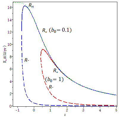
This model is a combination of two dominant universes, so there are two coincidence times: the earlier coincidence time in matter-dominated case and the later coincidence time in lambda-dominated universe. Hence the coincidence times can be found in two extreme limits. As wee see in Fig. 3, the later critical time is shown near $z=-1$ , while the earlier time is near $z\rightarrow\infty$ whose case is not shown here. When we extend $z$ infinitely, we will see that two horizons meet.

In the limit of $z+1\rightarrow\infty$ , the solution is approximately

(1+z)\approx\left(\frac{1}{2b_{0}H_{0}}\right)^{2}\frac{1}{\Omega_{\rm m0}},

(44)

which is the earlier coincidence time $t_{1}$ due to $\Omega_{\rm m0}$ . If we represent this time in terms of $t$ , we can see that this time is equal to $t_{\rm c}^{(m)}=(4b_{r}/3)^{3}t_{0}$ of the matter-dominated single-component universe with $\Omega_{\rm m0}=1$ . In the limit of $z+1\rightarrow 0$ , the solution is

(1+z)\approx(2b_{0}H_{0})\sqrt{\Omega_{\rm\Lambda 0}}

(45)

which is the late coincidence time $t_{2}$ due to $\Omega_{\rm\Lambda 0}$ . If we set $\Omega_{\rm\Lambda 0}=1$ , this time is equal to $t_{\rm c}^{(\Lambda)}=t_{0}-\ln(2H_{0}t_{0}b_{r})/H_{0}$ of the lambda-dominated single-component universe. The larger the size of the wormhole throat $b_{0}$ , the closer the later meeting time is to $z=-1$ . If the ratio $\Omega_{\rm m0}/\Omega_{\rm\Lambda 0}$ is larger, the coincidence time $t_{1}$ is earlier. The smaller the ratio, the later the coincidence time $t_{2}$ .

III.5 Past light cone and particle horizon distance

The past light cone is defined as a past null geodesics in the spacetime. The proper distance in the spacetime of the wormhole cosmological model is

d_{p}(t)=a(t)\int_{0}^{r}\left(1+\frac{b_{0}^{2}}{4r^{2}}\right)dr=a(t)r\left(1-\frac{b_{0}^{2}}{4r^{2}}\right)\equiv a(t)r^{*},

(46)

which is shortened to the factor of $(1-b_{0}^{2}/4r^{2})$ due to wormhole effect because of the range of the coordinate $r$ . The larger wormhole is subject to a more reduction in space near the origin. However, the null radial geodesic (constant $\theta,\phi$ ) is given by

dt^{2}=a^{2}\left(1+\frac{b_{0}^{2}}{4r^{2}}\right)^{2}dr^{2},

(47)

and the conformal time is just the proper distance along the null geodesic as

\int\frac{dt}{a}=\int_{0}^{r}\left(1+\frac{b_{0}^{2}}{4r^{2}}\right)dr=r^{*}.

(48)

As can be seen in Fig. 4, the null dashed line is the past light cone for the universe without wormhole in $r-\tau$ coordinates spacetime. However, the past light cone in wormhole cosmology is determined by the different proper time $r_{*}=r(1-b_{0}^{2}/4r^{2})$ instead of $r$ (Fig.4(a)). Thus the line of the null geodesic for wormhole cosmology is timelike solid line in the figure. If we eliminate the region $r<b_{0}/2$ and combine two solid lines, it becomes the past light cone for the wormhole universe. It is narrower than that in the universe without a wormhole whose null geodesic is in dashed line.

If they are represented together in $r_{*}-\tau$ coordinates spacetime in Fig. 4(b), the modified past light cone shows the null line $\tau=r_{*}$ and past light cone of the case without wormhole shows the spacelike line $\tau=r=\frac{1}{2}[r_{*}+\sqrt{R_{*}^{2}+b_{0}^{2}}]$ . The latter (the universe with wormhole) starts earlier by $\tau=b_{0}/2$ than the former (the universe without wormhole), as shown in Fig. 4(b). Of course, if we draw the past light cones in $(2+1)$ -dimensional spacetime with $r_{*}-\tau$ coordinates, they are null cone in the case with wormhole and spacelike cone in the case without wormhole, as shown in Fig. 4(c).

A Penrose diagram of the wormhole cosmological model is shown in Fig. 5. It is the just the case of curvature zero and matter-dominated universe. At the coordinate origin, there is a dynamical wormhole that starts at a time later than the initial singularity. The spacelike surface of coincidence time $t=t_{\rm c}$ is drawn in figure. We can think of the past light cones for several observers. When the observer such as $P^{\prime}$ is earlier than the generation of the wormhole, or the observer such as $P^{\prime\prime}$ is far from the wormhole, their past light cones will not pass through the wormhole. However, the past light cone of the observer such as $P$ who exists after the creation and near the wormhole, include a region of the other’s universe or a region far from the observer, because the past light cone of $P$ consists of the information from the same universe and the information from the other universe through the throat of the wormhole. Therefore, the past light cone after the time $t=t_{\rm c}$ is not defined unique way, in case of the travel-through-wormhole at least. As shown in the figure, the past light cone can be extended into another universe or far distant causally disconnected regions through the wormhole. The past light cone of the observer $P_{0}$ is the boundary between the case where it can pass through the wormhole and the case where it can not.

The particle horizon distance is determined from the distance from the observer to the end of the past light cone Harrison. In the following three cases there are problems with the existence of the particle horizon: (1) When the universe originates in the infinite past in conformal time, particle horizon does not exist Harrison. (2) In the case of the accelerating (de Sitter steady state, and $q>1$ ) universe of continual accelerated expansion, particle horizon does not exist Harrison. (3) In the universe with non-trivial topology such as wormhole cosmology, the distance of the past light cone is not unique. Thus the particle horizon distance is not determined in unique way for this universe with a wormhole. The distance of the past light cone from the observer to other universe by travel through the wormhole is quite different from the one in the same universe. When we think of a model with wormhole at the very early times, the two causally disconnected regions can be communicated with each other through the throat of the wormhole. This means that the horizon problem did not occur. This result is in accord with the Hochberg’s model hochberg.

For the universe of constant $\xi$ , deceleration parameter, with no wormholes, the particle horizon distance is $R_{\rm p}=R_{\rm H}/\xi$ and the speed of it is $dR_{\rm p}/dt=1+1/\xi$ in (16). Thus $R_{\rm p}>R_{\rm H}$ for matter-dominated universe and $R_{\rm p}=R_{\rm H}$ for radiation-dominated universe. However, in the case of wormhole cosmological model, the proper distance to the particle horizon is reduced by wormhole factor $(1-b_{0}^{2}/4r^{2})$ , after the generation of the wormhole, and the Hubble horizon is replaced by the apparent cosmological horizon. The effect of the wormhole factor on the proper distance is dominant near the wormhole, but there is a travel through the wormhole throat like the observer $P$ in Fig. 5. When the observer is far from the wormhole such as $P^{\prime\prime}$ , the observer’s past light cone does not pass the wormhole, and the particle horizon is still larger than the modified Hubble horizon $R_{+}$ . Therefore, we can say that the presence of a wormhole in our universe does not change the relationship between the particle horizon and the Hubble horizon, if only the observer is far from the wormhole sufficiently enough prevent from the travel through the wormhole throat.

IV summary and discussions

In this paper, we investigated the cosmological horizon of the wormhole cosmological model for matter-dominant universe and/or lambda. We checked the properties of the time dependencies of the apparent horizons and the role of wormhole in the universe. After the wormhole is created at Planck time with Planck size, the wormhole also expands along the scale factor. The apparent cosmological horizon, the modified Hubble horizon has the meaning of a boundary between observable and unobservable regions of the universe.

The observer’s past light cone depends on proper distance in the spacetime. The past light cones are examined for what happen in the model with a wormhole. Because the smaller-than-wormhole region is eliminated from the spacetime for the universe with a wormhole, the past light cone is narrower than the one in the universe without a wormhole. So the past light cone in the universe without a wormhole starts earlier than that in the universe with a wormhole in proper distance coordinates. Moreover, the travel-through-wormhole throat can shows a different way of communication from normal travel. Therefore, the particle horizon distance determined from the observer’s past light cone can not be defined unique way. For the case of the travel through the wormhole, the past light cone can be extended into another universe or far distant causally disconnected region. In this way we can say that the horizon problem does not occur in this wormhole cosmological model, because there were causal contact between two separated regions through wormhole mouth at very early times. When the observer is far from the wormhole or before generation of the wormhole, the particle horizon distance is the same as the wormhole-less case except that the proper distance is shortened by the wormhole factor after the generation of the wormhole.

We can think about the stability issue of the wormhole in the universe. As shown in the dynamics of the apparent horizons, the size of the wormhole throat varies with time and expands according to the scale factor. That is, the wormhole is unstable, even though our model does not allow the inflow. Such result have already been covered by Shinkai and Hayward Shinkai, which showed that a wormhole will collapse to black hole or expand to a huge size due to a normal or ghost matter inflows.

Another issue is the creation of a wormhole in the early time of the universe. Usually we consider the generation of wormholes in the early time, taking into consideration the quantum era and foams caused by the fluctuation of spacetime. In our model, instead of this, as we see, the construction of the wormhole was delayed by a very short time after big bang. In other words, the expansion rate of the scale factor is very fast, so a highly localized exotic matter for constructing a wormhole could not form any wormhole at the big bang time. Later, however, when the expansion rate of the universe falls down in a very short time, the wormhole and apparent cosmological horizons are created and expand along the scale factor. Even though there might be a question about the destruction of the wormhole structure due to the interaction between the background matter and the wormhole matter, the highly localized exotic matter maintains the wormhole and rapidly expands with scale factor without mixing with the background matter.

Acknowledgements.

This work was supported by National Research Foundation of Korea (NRF) funded by the Ministry of Education (2017-R1D1A1B03031081).

References

(1) Sung-Won Kim, Phys. Lett. B 780 (2018) 174: arXiv. 1801.07989.
(2) M. L. Mc Vittie, Mon. Not. R. Astron. Soc. 93 (1933) 315.
(3) Sung-Won Kim, Phys. Lett. A 166 (1992) 13.
(4) David Hochberg and Thomas W. Kepart, Phys. Rev. Lett. 70 (1993) 2665.
(5) Thomas A. Roman, Phys. Rev. D 47 (1993) 1370.
(6) Sung-Won Kim, Phys. Rev. D 53 (1996) 6889.
(7) Li-Xin Li, J. Geom. Phys. 40 (2001) 154.
(8) Pedro F. González-Díaz, Phys. Rev. D 68 (2003) 084016.
(9) B. Mirza, M. Eshaghi, and S. Dehdashti, Int. J. Mod. Phys. D 15 (2006) 1217.
(10) Ivana Bochiccio and Valerio Faraoni, Phys. Rev. D 82 (2010) 044040.
(11) M. Morris and K. S. Thorne, Am. J. Phys. 56 (1988) 395.
(12) Matt Visser, Phys. Rev. D 43 (1989) 3182.
(13) P.A.R. Ade et al. [Planck Collaboration], Astron. Astrophys. 594 (2016) A13.
(14) Edward Harrison, Astrophys. J. 383 (1991) 60. (2008) 024008.
(15) Hisa-aki Shinkai and Sean A. Hayward, Phys. Rev. D 66 (2002) 044005.