RMPflow: A Computational Graph for
Automatic Motion Policy Generation

We model motion as a second-order differential equation³³ 3 We assume the system has been feedback linearized. A torque-based setup can be similarly derived by setting the robot inertia matrix as the intrinsic metric on $\mathcal{C}$ Peters_AR_2008. of ${\ddot{\mathbf{q}}}=\pi(\mathbf{q},{\dot{\mathbf{q}}})$, where we call $\pi$ a motion policy and $(\mathbf{q},{\dot{\mathbf{q}}})$ the state. In contrast to an open-loop trajectory, which forms the basis of many motion planners, a motion policy expresses the entire continuous collection of its integral trajectories and therefore is robust to perturbations. Motion policies can model many adaptive behaviors, such as reactive obstacle avoidance DRCIntegratedSystemTodorov2013; 2017_rss_system or responses driven by planned Q-functions OptimalControlTheoryTodorov06, and their second-order formulation enables rich behavior that cannot be realized by the velocity-based approach liegeois1977automatic.

The geometry of motion has been considered by many planning and control algorithms. Geometrical modeling of task spaces is used in topological motion planning VijayakumarTopologyMotionPlanning2013, and motion optimization has leveraged Hessian to exploit the natural geometry of costs RatliffCHOMP2009; ToussaintTrajOptICML2009; Mukadam-ICRA-16; Dong-RSS-16. Ratliff et al. RIEMORatliff2015ICRA, e.g., use the workspace geometry inside a Gauss-Newton optimizer and generate natural obstacle-avoiding reaching motion through traveling along geodesics of curved spaces.

Geometry-aware motion policies were also developed in parallel in controls. OSC is the best example khatib1987unified. Unlike the planning approaches, OSC focuses on the internal geometry of the robot and considers only simple task-space geometry. It reshapes the workspace dynamics into a simple spring-mass-damper system with a constant inertia matrix, enforcing a form of Euclidean geometry in the task space. Variants of OSC have been proposed to consider different metrics Nakanishi_IJRR_2008; Peters_AR_2008; lo2016virtual, task hierarchies sentis2006whole; platt2011multiple, and non-stationary inputs IjspeertDMPs2013.

While these algorithms have led to many advances, we argue that their isolated focus on either the internal or the external geometry limits the performance. The planning approach fails to consider reactive dynamic behavior; the control approach cannot model the effects of velocity dependent metrics, which are critical to generating sensible obstacle avoidance motions, as discussed in the introduction. While the benefits of velocity dependent metrics was recently explored using RMPs ratliff2018riemannian, a systematic understanding is still an open question.

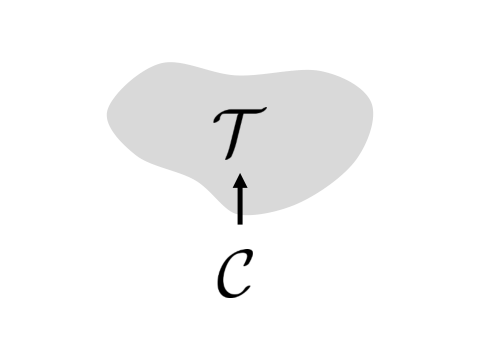
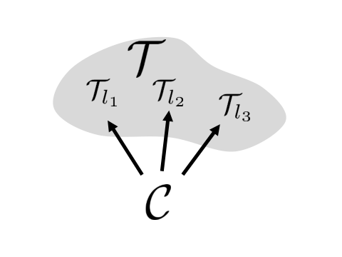
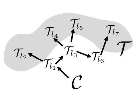
In most cases, the task-space manifold $\mathcal{T}$ is structured. In this paper, we consider the case where the task map $\psi$ can be expressed through a tree-structured composition of transformations $\{\psi_{e_{i}}\}$, where $\psi_{e_{i}}$ is the $i$th transformation. Fig. 1 illustrates some common examples. Each node denotes a manifold and each edge denotes a transformation. This family trivially includes the unstructured task space $\mathcal{T}$ (Fig. 1a) and the product manifold $\mathcal{T}=\mathcal{T}_{l_{1}}\times\dots\times\mathcal{T}_{l_{K}}$ (Fig. 1b), where $K$ is the number of subtasks. A more interesting example is the kinematic tree (Fig. 1c), where, e.g., the subtask spaces on the leaf nodes can describe the tracking and obstacle avoidance tasks along a multi-DOF robot.

The main motivation of explicitly handling the structure in the task map $\psi$ is two-fold. First, it allows RMPflow to exploit computation shared across different subtask maps. Second, it allows the user to focus on designing motion policies for each subtask individually, which is easier than directly designing a global policy for the entire task space $\mathcal{T}$. For example, $\mathcal{T}$ may describe the problem of humanoid walking, which includes staying balanced, scheduling contacts, and avoiding collisions. Directly parameterizing a policy to satisfy all these objectives can be daunting, whereas designing a policy for each subtask is more feasible.

Knowing the structure of the task map is not sufficient for consistently combining subtask policies: we require some geometric information about the motion policies’ behaviors ratliff2018riemannian. Toward this end, we adopt an abstract description of motion policies, called RMPs ratliff2018riemannian, for the nodes of the RMP-tree. Specifically, let $\mathcal{M}$ be an $m$-dimensional manifold with coordinate $\mathbf{x}\in\mathbb{R}^{m}$. The canonical form of an RMP on $\mathcal{M}$ is a pair $(\mathbf{a},\mathbf{M})^{\mathcal{M}}$, where $\mathbf{a}:\mathbb{R}^{m}\times\mathbb{R}^{m}\to\mathbb{R}^{m}$ is a continuous motion policy and $\mathbf{M}:\mathbb{R}^{m}\times\mathbb{R}^{m}\to\mathbb{R}_{+}^{m\times m}$ is a differentiable map. Borrowing terminology from mechanics, we call $\mathbf{a}(\mathbf{x},{\dot{\mathbf{x}}})$ the desired acceleration and $\mathbf{M}(\mathbf{x},{\dot{\mathbf{x}}})$ the inertia matrix at $(\mathbf{x},{\dot{\mathbf{x}}})$, respectively.⁴⁴ 4 Here we adopt a slightly different terminology from ratliff2018riemannian. We note that $\mathbf{M}$ and $\mathbf{f}$ do not necessarily correspond to the inertia and force of a physical mechanical system. $\mathbf{M}$ defines the directional importance of $\mathbf{a}$ when it is combined with other motion policies. Later in Section 4, we will show that $\mathbf{M}$ is closely related to Riemannian metric, which describes how the space is stretched along the curve generated by $\mathbf{a}$; when $\mathbf{M}$ depends on the state, the space becomes non-Euclidean. We additionally introduce a new RMP form, called the natural form. Given an RMP in its canonical form $(\mathbf{a},\mathbf{M})^{\mathcal{M}}$, the natural form is a pair $[\mathbf{f},\mathbf{M}]^{\mathcal{M}}$, where $\mathbf{f}=\mathbf{M}\mathbf{a}$ is the desired force map. While the transformation between these two forms may look trivial, their distinction will be useful later when we introduce the RMP-algebra.

The RMP-tree is the core data structure used by RMPflow. An RMP-tree is a directed tree, in which each node represents an RMP and its state, and each edge corresponds to a transformation between manifolds. The root node of the RMP-tree describes the global policy $\pi$ on $\mathcal{C}$, and the leaf nodes describe the local policies $\{\pi_{l_{i}}\}$ on $\{\mathcal{T}_{l_{i}}\}$. To illustrate, let us consider a node $u$ and its $K$ child nodes $\{v_{i}\}_{i=1}^{K}$. Suppose $u$ describes an RMP $[\mathbf{f},\mathbf{M}]^{\mathcal{M}}$ and $v_{i}$ describes an RMP $[\mathbf{f}_{i},\mathbf{M}_{i}]^{\mathcal{N}_{i}}$, where $\mathcal{N}_{i}=\psi_{e_{i}}(\mathcal{M})$ for some $\psi_{e_{i}}$. Then we write $u=((\mathbf{x},{\dot{\mathbf{x}}}),[\mathbf{f},\mathbf{M}]^{\mathcal{M}})$ and $v_{i}=((\mathbf{y}_{i},{\dot{\mathbf{y}}}_{i}),[\mathbf{f}_{i},\mathbf{M}_{i}]^{\mathcal{N}_{i}})$; the edge connecting $u$ and $v_{i}$ points from $u$ to $v_{i}$ along $\psi_{e_{i}}$. We will continue to use this example to illustrate how RMP-algebra propagates the information across the RMP-tree.

The RMP-algebra consists of three operators (pushforward, pullback, and resolve) to propagate information.⁵⁵ 5 Precisely it propagates the numerical values of RMPs and states at a particular time. They form the basis of the forward and backward passes for automatic policy generation, described in the next section.

1. 1.

   pushforward is the operator to forward propagate the state from a parent node to its child nodes. Using the previous example, given $(\mathbf{x},{\dot{\mathbf{x}}})$ from $u$, it computes $(\mathbf{y}_{i},{\dot{\mathbf{y}}}_{i})=(\psi_{e_{i}}(\mathbf{x}),\mathbf{J}_{i}(\mathbf{x}){\dot{\mathbf{x}}})$ for each child node $v_{i}$, where $\mathbf{J}_{i}=\partial_{\mathbf{x}}\psi_{e_{i}}$ is a Jacobian matrix. The name “pushforward” comes from the linear transformation of tangent vector ${\dot{\mathbf{x}}}$ to the image tangent vector ${\dot{\mathbf{y}}}_{i}$.

2. 2.

   pullback is the operator to backward propagate the natural-formed RMPs from the child nodes to the parent node. It is done by setting $[\mathbf{f},\mathbf{M}]^{\mathcal{M}}$ with

   $\displaystyle\textstyle\mathbf{f}=\sum_{i=1}^{K}\mathbf{J}_{i}^{\top}(\mathbf{f}_{i}-\mathbf{M}_{i}\dot{\mathbf{J}}_{i}{\dot{\mathbf{x}}})\qquad\text{and}\qquad\mathbf{M}=\sum_{i=1}^{K}\mathbf{J}_{i}^{\top}\mathbf{M}_{i}\mathbf{J}_{i}$

   (1)

   The name “pullback” comes from the linear transformations of the cotangent vector (1-form) $\mathbf{f}_{i}-\mathbf{M}_{i}\dot{\mathbf{J}_{i}}{\dot{\mathbf{x}}}$ and the inertia matrix (2-form) $\mathbf{M}_{i}$. In summary, velocities can be pushfowarded along the direction of $\psi_{i}$, and forces and inertial matrices can be pullbacked in the opposite direction.

   To gain more intuition of pullback, we write pullback in the canonical form of RMPs. It can be shown that the canonical form $(\mathbf{a},\mathbf{M})^{\mathcal{M}}$ of the natural form $[\mathbf{f},\mathbf{M}]^{\mathcal{M}}$ above is the solution to a least-squared problem:

   $\displaystyle\mathbf{a}$

   $\displaystyle=\textstyle\argmin_{\mathbf{a}^{\prime}}\frac{1}{2}\sum_{i=1}^{K}\|\mathbf{J}_{i}\mathbf{a}^{\prime}+\dot{\mathbf{J}}_{i}{\dot{\mathbf{x}}}-\mathbf{a}_{i}\|_{\mathbf{M}_{i}}^{2}$

   (2)

   where $\mathbf{a}_{i}=\mathbf{M}_{i}^{\dagger}\mathbf{f}_{i}$ and $\|\cdot\|_{\mathbf{M}_{i}}^{2}=\left\langle\cdot,\mathbf{M}_{i}\cdot\right\rangle$. Because ${\ddot{\mathbf{y}}}_{i}=\mathbf{J}_{i}{\ddot{\mathbf{x}}}+\dot{\mathbf{J}}_{i}{\dot{\mathbf{x}}}$, pullback attempts to find an $\mathbf{a}$ that can realize the desired accelerations $\{\mathbf{a}_{i}\}$ while trading off approximation errors with an importance weight defined by the inertia matrix $\mathbf{M}_{i}(\mathbf{y}_{i},{\dot{\mathbf{y}}}_{i})$. The use of state dependent importance weights is a distinctive feature of RMPflow. It allows RMPflow to activate different RMPs according to both configuration and velocity (see Section 3.6 for examples). Finally, we note that the pullback operator defined in this paper is slightly different from the original definition given in ratliff2018riemannian, which ignores the term $\dot{\mathbf{J}}_{i}{\dot{\mathbf{x}}}$ in (2). While ignoring $\dot{\mathbf{J}}_{i}{\dot{\mathbf{x}}}$ does not necessary destabilize the system lo2016virtual, its inclusion is critical to implement consistent policy behaviors.

3. 3.

   resolve is the last operator of RMP-algebra. It maps an RMP from its natural form to its canonical form. Given $[\mathbf{f},\mathbf{M}]^{\mathcal{M}}$, it outputs $(\mathbf{a},\mathbf{M})^{\mathcal{M}}$ with $\mathbf{a}=\mathbf{M}^{\dagger}\mathbf{f}$, where $\dagger$ denotes Moore-Penrose inverse. The use of pseudo-inverse is because in general the inertia matrix is only positive semi-definite. Therefore, we also call the natural form of $[\mathbf{f},\mathbf{M}]^{\mathcal{M}}$ the unresolved form, as potentially it can be realized by multiple RMPs in the canonical form.

Now we show how RMPflow uses the RMP-tree and RMP-algebra to generate a global policy $\pi$ on $\mathcal{C}$. Suppose each subtask policy is provided as an RMP. First, we construct an RMP-tree with the same structure as $\psi$, where we assign subtask RMPs as the leaf nodes and the global RMP $[\mathbf{f}_{r},\mathbf{M}_{r}]^{\mathcal{C}}$ as the root node. With the RMP-tree specified, RMPflow can perform automatic policy generation. At every time instance, it first performs a forward pass: it recursively calls pushforward from the root node to the leaf nodes to update the state information in each node in the RMP-tree. Second, it performs a backward pass: it recursively calls pullback from the leaf nodes to the root node to back propagate the values of the RMPs in the natural form, and finally calls resolve at the root node to transform the global RMP $[\mathbf{f}_{r},\mathbf{M}_{r}]^{\mathcal{C}}$ into its canonical form $(\mathbf{a}_{r},\mathbf{M}_{r})^{\mathcal{C}}$ for policy execution (i.e. setting $\pi(\mathbf{q},{\dot{\mathbf{q}}})=\mathbf{a}_{r}$).

The process of policy generation of RMPflow uses the tree structure for computational efficiency. For $K$ subtasks, it has time complexity $O(K)$ in the worst case as opposed to $O(K\log K)$ of a naive implementation which does not exploit the tree structure. Furthermore, all computations of RMPflow are carried out using matrix-multiplications, except for the final resolve call, because the RMPs are expressed in the natural form in pullback instead of the canonical form suggested originally in ratliff2018riemannian. This design makes RMPflow numerically stable, as only one matrix inversion $\mathbf{M}_{r}^{\dagger}\mathbf{f}_{r}$ is performed at the root node with both $\mathbf{f}_{r}$ and $\mathbf{M}_{r}$ in the span of the same Jacobian matrix due to pullback.

We give a quick overview of some RMPs useful in practice (a complete discussion of these RMPs are postponed to Appendix D). We recall from (2) that $\mathbf{M}$ dictates the directional importance of an RMP.

We define a new family of dynamics useful to specify RMPs on manifolds. Let manifold $\mathcal{M}$ be $m$-dimensional with chart $(\mathcal{M},\mathbf{x})$. Let $\mathbf{G}:\mathbb{R}^{m}\times\mathbb{R}^{m}\to\mathbb{R}^{m\times m}_{+}$, $\mathbf{B}:\mathbb{R}^{m}\times\mathbb{R}^{m}\to\mathbb{R}^{m\times m}_{+}$, and $\Phi:\mathbb{R}^{m}\to\mathbb{R}$. The tuple $(\mathcal{M},\mathbf{G},\mathbf{B},\Phi)$ is called a GDS if and only if

where $\bm{\Xi}_{\mathbf{G}}(\mathbf{x},{\dot{\mathbf{x}}})\coloneqq\frac{1}{2}\sum_{i=1}^{m}\dot{x}_{i}\partial_{{\dot{\mathbf{x}}}}\mathbf{g}_{i}(\mathbf{x},{\dot{\mathbf{x}}})$, $\bm{\xi}_{\mathbf{G}}(\mathbf{x},{\dot{\mathbf{x}}})\coloneqq\overset{\lower 0.81949pt\hbox{$\scriptscriptstyle\mathbf{x}$}}{\mathbf{G}}(\mathbf{x},{\dot{\mathbf{x}}}){\dot{\mathbf{x}}}-\frac{1}{2}\nabla_{\mathbf{x}}({\dot{\mathbf{x}}}^{\top}\mathbf{G}(\mathbf{x},{\dot{\mathbf{x}}}){\dot{\mathbf{x}}})$, and $\overset{\lower 0.81949pt\hbox{$\scriptscriptstyle\mathbf{x}$}}{\mathbf{G}}(\mathbf{x},{\dot{\mathbf{x}}})\coloneqq[\partial_{\mathbf{x}}\mathbf{g}_{i}(\mathbf{x},{\dot{\mathbf{x}}}){\dot{\mathbf{x}}}]_{i=1}^{m}$. We refer to $\mathbf{G}(\mathbf{x},{\dot{\mathbf{x}}})$ as the metric matrix, $\mathbf{B}(\mathbf{x},{\dot{\mathbf{x}}})$ as the damping matrix, and $\Phi(\mathbf{x})$ as the potential function which is lower-bounded. In addition, we define $\mathbf{M}(\mathbf{x},{\dot{\mathbf{x}}})\coloneqq\mathbf{G}(\mathbf{x},{\dot{\mathbf{x}}})+\bm{\Xi}_{\mathbf{G}}(\mathbf{x},{\dot{\mathbf{x}}})$ as the inertia matrix, which can be asymmetric. We say a GDS is non-degenerate if $\mathbf{M}(\mathbf{x},{\dot{\mathbf{x}}})$ is nonsingular. We will assume (3) is non-degenerate so that it uniquely defines a differential equation and discuss the general case in Appendix A. $\mathbf{G}(\mathbf{x},{\dot{\mathbf{x}}})$ induces a metric of ${\dot{\mathbf{x}}}$, measuring its length as $\frac{1}{2}{\dot{\mathbf{x}}}^{\top}\mathbf{G}(\mathbf{x},{\dot{\mathbf{x}}}){\dot{\mathbf{x}}}$. When $\mathbf{G}(\mathbf{x},{\dot{\mathbf{x}}})$ depends on $\mathbf{x}$ and ${\dot{\mathbf{x}}}$, it also induces the curvature terms $\bm{\Xi}(\mathbf{x},{\dot{\mathbf{x}}})$ and $\bm{\xi}(\mathbf{x},{\dot{\mathbf{x}}})$. In a particular case when $\mathbf{G}(\mathbf{x},{\dot{\mathbf{x}}})=\mathbf{G}(\mathbf{x})$, the GDSs reduce to the widely studied simple mechanical systems (SMSs) bullo2004geometric, $\mathbf{M}(\mathbf{x}){\ddot{\mathbf{x}}}+\mathbf{C}(\mathbf{x},{\dot{\mathbf{x}}}){\dot{\mathbf{x}}}+\nabla_{\mathbf{x}}\Phi(\mathbf{x})=-\mathbf{B}(\mathbf{x},{\dot{\mathbf{x}}}){\dot{\mathbf{x}}}$; in this case $\mathbf{M}(\mathbf{x})=\mathbf{G}(\mathbf{x})$ and the Coriolis force $\mathbf{C}(\mathbf{x},{\dot{\mathbf{x}}}){\dot{\mathbf{x}}}$ is equal to $\bm{\xi}_{\mathbf{G}}(\mathbf{x},{\dot{\mathbf{x}}})$. The extension to velocity-dependent $\mathbf{G}(\mathbf{x},{\dot{\mathbf{x}}})$ is important and non-trivial. As discussed in Section 3.6, it generalizes the dynamics of classical rigid-body systems, allowing the space to morph according to the velocity direction.

As its name suggests, GDSs possess geometric properties. Particularly, when $\mathbf{G}(\mathbf{x},{\dot{\mathbf{x}}})$ is invertible, the left-hand side of (3) is related to a quantity $\mathbf{a}_{\mathbf{G}}={\ddot{\mathbf{x}}}+\mathbf{G}(\mathbf{x},{\dot{\mathbf{x}}})^{-1}(\bm{\Xi}_{\mathbf{G}}(\mathbf{x},{\dot{\mathbf{x}}}){\ddot{\mathbf{x}}}+\bm{\xi}_{\mathbf{G}}(\mathbf{x},{\dot{\mathbf{x}}}))$, known as the geometric acceleration (cf. Section 4.4). In short, we can think of (3) as setting $\mathbf{a}_{\mathbf{G}}$ along the negative natural gradient $-\mathbf{G}(\mathbf{x},{\dot{\mathbf{x}}})^{-1}\nabla_{\mathbf{x}}\Phi(\mathbf{x})$ while imposing damping $-\mathbf{G}(\mathbf{x},{\dot{\mathbf{x}}})^{-1}\mathbf{B}(\mathbf{x},{\dot{\mathbf{x}}}){\dot{\mathbf{x}}}$.

Earlier, we mentioned that by tracking the geometry in pullback in (1), the task properties can be preserved. Here, we formalize the consistency of RMPflow as a closure of differential equations, named structured GDSs. Structured GDSs augment GDSs with information on how the metric matrix factorizes. Suppose $\mathbf{G}$ has a structure $\mathcal{S}$ that factorizes $\mathbf{G}(\mathbf{x},{\dot{\mathbf{x}}})=\mathbf{J}(\mathbf{x})^{\top}\mathbf{H}(\mathbf{y},{\dot{\mathbf{y}}})\mathbf{J}(\mathbf{x})$, where $\mathbf{y}:\mathbf{x}\mapsto\mathbf{y}(\mathbf{x})\in\mathbb{R}^{n}$ and $\mathbf{H}:\mathbb{R}^{n}\times\mathbb{R}^{n}\to\mathbb{R}^{n\times n}_{+}$, and $\mathbf{J}(\mathbf{x})=\partial_{\mathbf{x}}\mathbf{y}$. We say the tuple $(\mathcal{M},\mathbf{G},\mathbf{B},\Phi)_{\mathcal{S}}$ is a structured GDS if and only if

where $\bm{\eta}_{\mathbf{G};\mathcal{S}}(\mathbf{x},{\dot{\mathbf{x}}})\coloneqq\mathbf{J}(\mathbf{x})^{\top}(\bm{\xi}_{\mathbf{H}}(\mathbf{y},{\dot{\mathbf{y}}})+(\mathbf{H}(\mathbf{y},\dot{\mathbf{y}})+\bm{\Xi}_{\mathbf{H}}(\mathbf{y},{\dot{\mathbf{y}}}))\dot{\mathbf{J}}(\mathbf{x},{\dot{\mathbf{x}}}){\dot{\mathbf{x}}})$. Note the metric and factorization in combination defines $\bm{\eta}_{\mathbf{G};\mathcal{S}}$. As a special case, GDSs are structured GDSs with a trivial structure (i.e. $\mathbf{y}=\mathbf{x}$). Also, structured GDSs reduce to GDSs (i.e. the structure offers no extra information) if $\mathbf{G}(\mathbf{x},{\dot{\mathbf{x}}})=\mathbf{G}(\mathbf{x})$, or if $n,m=1$ (cf. Appendix B.1). Given two structures, we say $\mathcal{S}_{a}$ preserves $\mathcal{S}_{b}$ if $\mathcal{S}_{a}$ has the factorization (of $\mathbf{H}$) made by $\mathcal{S}_{b}$. In Section 4.4, we will show that structured GDSs are related to a geometric object, pullback connection, which turns out to be the coordinate-free version of pullback.

To show the closure property, we consider a parent node on $\mathcal{M}$ with $K$ child nodes on $\{\mathcal{N}_{i}\}_{i=1}^{K}$. We note that $\mathbf{G}_{i}$ and $\mathbf{B}_{i}$ can be functions of both $\mathbf{y}_{i}$ and ${\dot{\mathbf{y}}}_{i}$.

By the closure property above, we analyze the stability of RMPflow when the leaf nodes are (structured) GDSs. For compactness, we will abuse the notation to write $\mathbf{M}=\mathbf{M}_{r}$. Suppose $\mathbf{M}$ is nonsingular and let $(\mathcal{C},\mathbf{G},\mathbf{B},\Phi)_{\mathcal{S}}$ be the resultant structured GDS at the root node. We consider a Lyapunov candidate $V(\mathbf{q},{\dot{\mathbf{q}}})=\frac{1}{2}{\dot{\mathbf{q}}}^{\top}\mathbf{G}(\mathbf{q},{\dot{\mathbf{q}}}){\dot{\mathbf{q}}}+\Phi(\mathbf{q})$ and derive its rate using properties of structured GDSs.

To show the stability of RMPflow, we need to further check when the assumptions in Corollary 2 hold. The condition $\mathbf{B}(\mathbf{q},{\dot{\mathbf{q}}})\succ 0$ is easy to satisfy: by Theorem 4.1, $\mathbf{B}(\mathbf{q},{\dot{\mathbf{q}}})\succeq 0$; to strictly ensure definiteness, we can copy $\mathcal{C}$ into an additional child node with a (small) positive-definite damping matrix. The condition on $\mathbf{G}(\mathbf{q},{\dot{\mathbf{q}}})\succ 0$ can be satisfied similarly. In addition, we need to verify the assumption that $\mathbf{M}$ is nonsingular. Here we provide a sufficient condition. When satisfied, it implies the global stability of RMPflow.

We now discuss the coordinate-free geometric properties of $(\mathcal{C},\mathbf{G},\mathbf{B},\Phi)_{\mathcal{S}}$ generated by RMPflow. Due to space constraint, we only summarize the results (please see Appendix B.4 and, e.g., lee2009manifolds). Here we assume that $\mathbf{G}$ is positive-definite.

We first present the coordinate-free version of GDSs (i.e. the structure is trivial) by using a geometric object called affine connection, which defines how tangent spaces on a manifold are related. Let $T\mathcal{C}$ denote the tangent bundle of $\mathcal{C}$, which is a natural manifold to describe the state space. We first show that a GDS on $\mathcal{C}$ can be written in terms of a unique, asymmetric affine connection ${}^{\scriptstyle G}{\nabla}$ that is compatible with a Riemannian metric $G$ (defined by $\mathbf{G}$) on $T\mathcal{C}$. It is important to note that $G$ is defined on $T\mathcal{C}$ not the original manifold $\mathcal{C}$. As the metric matrix in a GDS can be velocity dependent, we need a larger manifold.

Next we present a coordinate-free representation of RMPflow.

While here we focus on the special case of RMPflow with GDSs, this family already covers a wide range of reactive policies commonly used in practice. For example, when the task metric is Euclidean (i.e. constant), RMPflow recovers OSC (and its variants) khatib1987unified; sentis2006whole; Peters_AR_2008; UdwadiaGaussPrincipleControl2003; lo2016virtual. When the task metric is only configuration dependent, RMPflow can be viewed as performing energy shaping to combine multiple SMSs in geometric control bullo2004geometric. Further, RMPflow allows using velocity dependent metrics, generating behaviors all those previous rigid mechanics-based approaches fail to model. We also note that RMPflow can be easily modified to incorporate exogenous time-varying inputs (e.g. forces to realize impedance control albu2002cartesian or learned perturbations as in DMPs IjspeertDMPs2013). In computation, the structure of RMPflow in natural-formed RMPs resembles the classical Recursive Newton-Euler algorithm walker1982efficient; Featherstone08 (see Appendix C). Alternatively, the canonical form of RMPflow in (2) resembles Gauss’ Principle Peters_AR_2008; UdwadiaGaussPrincipleControl2003, but with a curvature correction $\bm{\Xi}_{\mathbf{G}}$ on the inertia matrix (suggested by Theorem 4.1) to account for velocity dependent metrics. Thus, we can view RMPflow as a natural generalization of these approaches to a broader class of non-Euclidean behaviors.

References

- (1) Rimon, E., Koditschek, D.: The construction of analytic diffeomorphisms for exact robot navigation on star worlds. Transactions of the American Mathematical Society 327(1), 71–116 (1991)
- (2) Ratliff, N., Toussaint, M., Schaal, S.: Understanding the geometry of workspace obstacles in motion optimization. In: IEEE International Conference on Robotics and Automation (ICRA) (2015)
- (3) Ivan, V., Zarubin, D., Toussaint, M., Komura, T., Vijayakumar, S.: Topology-based representations for motion planning and generalization in dynamic environments with interactions. International Journal of Robotics Research (IJRR) 32(9-10), 1151–1163 (2013)
- (4) Watterson, M., Liu, S., Sun, K., Smith, T., Kumar, V.: Trajectory optimization on manifolds with applications to SO(3) and R3XS2. In: Robotics: Science and Systems (RSS) (2018)
- (5) Toussaint, M.: Robot trajectory optimization using approximate inference. In: ICML. pp. 1049–1056 (2009)
- (6) LaValle, S.M.: Planning Algorithms. Cambridge University Press, Cambridge, U.K. (2006), available at http://planning.cs.uiuc.edu/
- (7) Karaman, S., Frazzoli, E.: Sampling-based algorithms for optimal motion planning. International Journal of Robotics Research (IJRR) 30(7), 846–894 (2011), http://arxiv.org/abs/1105.1186
- (8) Gammell, J.D., Srinivasa, S.S., Barfoot, T.D.: Batch Informed Trees (BIT*): Sampling-based optimal planning via the heuristically guided search of implicit random geometric graphs. In: IEEE International Conference on Robotics and Automation (ICRA) (2015)
- (9) Mukadam, M., Dong, J., Yan, X., Dellaert, F., Boots, B.: Continuous-time Gaussian process motion planning via probabilistic inference. arXiv preprint arXiv:1707.07383 (2017)
- (10) Khatib, O.: A unified approach for motion and force control of robot manipulators: The operational space formulation. IEEE Journal on Robotics and Automation 3(1), 43–53 (1987)
- (11) Peters, J., Mistry, M., Udwadia, F.E., Nakanishi, J., Schaal, S.: A unifying framework for robot control with redundant DOFs. Autonomous Robots 1, 1–12 (2008)
- (12) Udwadia, F.E.: A new perspective on the tracking control of nonlinear structural and mechanical systems. Proceedings of the Royal Society of London A: Mathematical, Physical and Engineering Sciences 459(2035), 1783–1800 (2003), http://rspa.royalsocietypublishing.org/content/459/2035/1783
- (13) Kappler, D., Meier, F., Issac, J., Mainprice, J., Garcia Cifuentes, C., Wüthrich, M., Berenz, V., Schaal, S., Ratliff, N., Bohg, J.: Real-time perception meets reactive motion generation. IEEE Robotics and Automation Letters 3(3), 1864–1871 (2018), https://arxiv.org/abs/1703.03512
- (14) Mukadam, M., Cheng, C.A., Yan, X., Boots, B.: Approximately optimal continuous-time motion planning and control via probabilistic inference. In: IEEE International Conference on Robotics and Automation (ICRA) (2017)
- (15) Bullo, F., Lewis, A.D.: Geometric control of mechanical systems: modeling, analysis, and design for simple mechanical control systems, vol. 49. Springer Science & Business Media (2004)
- (16) Ratliff, N.D., Issac, J., Kappler, D., Birchfield, S., Fox, D.: Riemannian motion policies. arXiv preprint arXiv:1801.02854 (2018)
- (17) Walker, M.W., Orin, D.E.: Efficient dynamic computer simulation of robotic mechanisms. Journal of Dynamic Systems, Measurement, and Control 104(3), 205–211 (1982)
- (18) Albu-Schaffer, A., Hirzinger, G.: Cartesian impedance control techniques for torque controlled light-weight robots. In: IEEE International Conference on Robotics and Automation (ICRA). vol. 1, pp. 657–663 (2002)
- (19) Sentis, L., Khatib, O.: A whole-body control framework for humanoids operating in human environments. In: IEEE International Conference on Robotics and Automation (ICRA). pp. 2641–2648 (2006)
- (20) Lo, S.Y., Cheng, C.A., Huang, H.P.: Virtual impedance control for safe human-robot interaction. Journal of Intelligent & Robotic Systems 82(1), 3–19 (2016)
- (21) Erez, T., Lowrey, K., Tassa, Y., Kumar, V., Kolev, S., Todorov, E.: An integrated system for real-time model-predictive control of humanoid robots. In: IEEE/RAS International Conference on Humanoid Robots (2013)
- (22) Todorov, E.: Optimal control theory. In Bayesian Brain: Probabilistic Approaches to Neural Coding pp. 269–298 (2006)
- (23) Liegeois, A.: Automatic supervisory control of the configuration and behaviour of multibody mechanisms. IEEE Transactions on Systems, Man and Cybernetics 7(12), 868–871 (1977)
- (24) Ratliff, N., Zucker, M., Bagnell, J.A.D., Srinivasa, S.: CHOMP: Gradient optimization techniques for efficient motion planning. In: IEEE International Conference on Robotics and Automation (ICRA) (2009)
- (25) Mukadam, M., Yan, X., Boots, B.: Gaussian process motion planning. In: IEEE Conference on Robotics and Automation (ICRA) (2016)
- (26) Dong, J., Mukadam, M., Dellaert, F., Boots, B.: Motion planning as probabilistic inference using Gaussian processes and factor graphs. In: Robotics: Science and Systems (RSS) (2016)
- (27) Nakanishi, J., Cory, R., Mistry, M., Peters, J., Schaal, S.: Operational space control: A theoretical and empirical comparison. International Journal of Robotics Research (IJRR) 6, 737–757 (2008)
- (28) Platt, R., Abdallah, M.E., Wampler, C.W.: Multiple-priority impedance control. In: IEEE International Conference on Robotics and Automation (ICRA). pp. 6033–6038. Citeseer (2011)
- (29) Ijspeert, A.J., Nakanishi, J., Hoffmann, H., Pastor, P., Schaal, S.: Dynamical movement primitives: Learning attractor models for motor behaviors. Neural Computation 25(2), 328–373 (Feb 2013)
- (30) Lewis, A.D.: The geometry of the maximum principle for affine connection control systems (2000)
- (31) Khalil, H.K.: Noninear systems. Prentice-Hall, New Jersey 2(5), 5–1 (1996)
- (32) Lee, J.M., Chow, B., Chu, S.C., Glickenstein, D., Guenther, C., Isenberg, J., Ivey, T., Knopf, D., Lu, P., Luo, F., et al.: Manifolds and differential geometry. Topology 643, 658 (2009)
- (33) Featherstone, R.: Rigid Body Dynamics Algorithms. Springer (2008)
- (34) Schmidt, T., Newcombe, R., Fox, D.: DART: Dense articulated real-time tracking with consumer depth cameras. Autonomous Robots 39(3) (2015)
- (35) Taylor, J.R.: Classical Mechanics. University Science Books (2005)
- (36) Udwadia, F.E., Kalaba, R.E.: Analytical Dynamics: A New Approach. Cambridge University Press (1996)
Appendices
Appendix A Geometric Dynamical Systems
Here we summarize details and properties of GDSs introduced in Section 4.1.
A.1 From Geometric Mechanics to GDSs
Our study of GDSs is motivated by geometric mechanics. Many formulations of mechanics exist, including Lagrangian mechanics ClassicalMechanicsTaylor05 and the aforementioned Gauss’s Principle of Least Constraint udwadia1996analytical—–They are all equivalent, implicitly sharing the same mathematical structure. In that sense, geometric mechanics, which models physical systems as geodesic flow on Riemannian manifolds, is the most explicit of these, revealing directly the underlying manifold structure and connecting to the broad mathematical tool set from Riemannian geometry. These connections enable us here to generalize beyond the previous simple mechanical systems studied in bullo2004geometric to non-classical systems that more naturally describe robotic behaviors with non-Euclidean geometric properties.
A.2 Degenerate GDSs
Let us recall the definition of GDSs.
Definition 1.
Let and let and be differentiable. We say the tuple is a GDS if