Fast error–controlling MOID computation for confocal elliptic orbitsJournal: Astronomy and Computing
Abstract
We present an algorithm to compute the minimum orbital intersection distance (MOID), or global minimum of the distance between the points lying on two Keplerian ellipses. This is achieved by finding all stationary points of the distance function, based on solving an algebraic polynomial equation of th degree. The algorithm tracks numerical errors appearing on the way, and treats carefully nearly degenerate cases, including practical cases with almost circular and almost coplanar orbits. Benchmarks confirm its high numeric reliability and accuracy, and that regardless of its error–controlling overheads, this algorithm pretends to be one of the fastest MOID computation methods available to date, so it may be useful in processing large catalogs.
Keywords:
close encounters , near-Earth asteroids , NEOs , catalogs , computational methods1 Introduction
The MOID parameter, or the minimum distance between points on two Keplerian orbits, has an important value in various Solar System studies. It measures the closeness of two trajectories in the space, and hence ascertains whether two bodies have a risk to collide. For example, if MOID appeared below the sum of radii of two bodies than such bodies may avoid a collision only if they orbit in a mean-motion resonance, or via a perturbating effect that may increase the MOID to a safe level before the bodies could actually collide. Otherwise, the bodies will necessarily collide in some future.
Therefore, computing the MOID is very old task with an application to Potentially Hazardous Objects (PHOs) and Near-Earth Asteroids (NEAs).
This problem is investigated over decades already, see e.g. (Sitarski 1968; Dybczyński et al. 1986) and more recent works by Armellin et al. 2010; Hedo et al. 2018.
The MOID is a minimum of some distance or distance-like function that depends on two arguments, determining positions on two orbits. The methods of finding the minima of can be split in several general cathegories, depending on the dimensionality of the optimization task to be solved. This depends on how much work is pre-computed analytically.
- 1.
Global optimization in 2D. As an ultimately simple example this includes e.g. the 2D brute-force (exhaustive) search of on a 2D grid. Thanks to the existence of rigorous and finite upper limits on the gradient of , which appears to be a trigonometric polynomial, we can always limit the finite difference by and . Thanks to such error predictability, algorithms of the 2D class appear the most reliable ones, because we can always determine the MOID, along with the orbital positions and , to any desired accuracy. An advanced method based on the 2D global optimization of , which includes high-order Taylor models and interval arithmetics, was presented by Armellin et al. 2010. Nevertheless, even advanced methods of this type cannot be fast due to the need of considering 2D domains.
- 2.
1D optimization. Here we eliminate from the numeric search by solving it from an analytic equation. The remaining orbital position is determined by numeric optimization of the 1D function . In general, this is faster than 2D minimization, but the derivative of is no longer bounded, because may turn infinite sometimes. Such cases may appear even for very simple circular orbits. Therefore, in general this method cannot provide a strict mathematical guarantee of the desired numerical accuracy. However, it appears more reliable than the methods of the next class. The SDG method discussed by Hedo et al. 2018 basically belongs to this class.
- 3.
Methods of the 0D class, in which both and are solved for rather than found by numeric optimization. This includes the method by Kholshevnikov and Vassiliev 1999b and by Gronchi 2002; Gronchi 2005, because they do not explicitly deal with any numeric optimization at all. The task is analytically reduced to solving a nonlinear equation with respect to and then express also analytically. Methods of this class are ultimately fast but relatively vulnerable to loosing roots due to numerical errors (in nearly degenerate cases). This effect becomes important because the equation for is quite complicated and subject to round-off errors. Also, this equation often have close (almost multiple) roots that are always difficult for numeric processing.
Here we present an efficient numeric implementation of the algebraic approach presented by Kholshevnikov and Vassiliev 1999b, similar to the one presented by Gronchi 2002; Gronchi 2005. This method belongs to the fast 0D class. It is based on analytic determination of all the critical points of the distance function, , augmented with an algebraic elimination of one of the two positional variables. Mathematically, the problem is reduced to a single polynomial equation of th degree with respect to one of the eccentric anomalies.
Recently, Hedo et al. 2018 suggested a method that does not rely on necessary determination of all the stationary points for the distance. It basically splits the problem in two tasks of 1D optimization, so this method belongs to the 1D class. Nevertheless, it proved per cent faster than the 0D Gronchi algorithm, according to the benchmarks. Though the performance differences appeared relatively moderate, there were revealed occurences when the Gronchi’s code suffered from numeric errors, reporting a wrong value for the MOID. Therefore, in this task the numeric reliability of the method is no less important than just the computing speed.
Direct implementation of the methods by Kholshevnikov and Vassiliev 1999b and Gronchi 2002 might be vulnerable, because finding roots of a high-degree polynomial might be a numerical challenge sometimes. When dealing with large asteroid catalogs, various almost-degenerate cases appear sometimes, if the equations to be solved contain almost-double or almost-multiple roots. Such roots are difficult to be estimated accurately, because they are sensitive to numeric errors (even if there were no errors in the input orbital elements). Moreover, we have a risk of ambiguity: if the polynomial has two or more very close real roots then numeric errors may result in moving them to the complex plane entirely, so that we may wrongly conclude that there are no such real roots at all. Such effect of lost of real roots may potentially result in overestimating the MOID, i.e. it may appear that we lost exactly the solution corresponding to the global minimum of the distance. This issue can be solved by paying attention not only to the roots formally identified as real, but also to all complex-valued roots that appear suspiciously close to the real axis. To define formally what means ‘suspiciously close’ we need to estimate numeric error attached to a given root, not just its formal value.
In other words, our task assignes an increased role to the numeric stability of the computation, because errors are known to dramatically increase when propagating through mathematical degeneracies. This motivated us to pay major attention to error control when implementing the method by Kholshevnikov and Vassiliev 1999b in a numerical algorithm.
The structure of the paper is as follows. In Sect. 2, we give some mathematical framework that our algorithm relies upon. Sect. 3 describes the numeric algorithm itself. Sect. 4 contains some guidelines on how to select meaningful error tolerances for our algorithm. Sect. 5 presents its performance tests. In Sect. 6, we describe several auxiliary tools included in our MOID library.
The C++ source code of our MOID library named distlink is available for download at http://sourceforge.net/projects/distlink.
2 Mathematical setting
Consider two confocal elliptic orbits: determined by the five geometric Keplerian elements , and determined analogously by the same variables with a stroke. Our final task is to find the minimum of the distance between two points lying on the corresponding orbits, and the orbital positions where this minimum is attained (here stands for the eccentric anomaly). According to Kholshevnikov and Vassiliev 1999b, this problem is reduced to solving for the roots of a trigonometric polynomial of minimum possible algebraic degree (trigonometric degree ). It is expressed in the following form:
| (1) |
where
| (2) |
and , . The quantities , , , represent pairwise scalar products of the vectors and :
| (3) |
with analogous definitions for and .
When all the roots of are found, for each we can determine the second position from
| (4) |
where
| (5) |
The sign of should be chosen to satisfy
| (6) |
so there is only a single value of that corresponds to a particular solution for .
Finally, after both the orbital positions and were determined, the squared distance between these points is , where
| (7) |
Therefore, our general computation scheme should look as follows: (i) find all real roots of ; (ii) for each solution of determine its corresponding ; (iii) for each such pair compute ; and (iv) among these values of select the minimum one. This will give us the required MOID estimate. As we can see, the most difficult step is finding all real roots of the trigonometric polynomial , while the rest of the work is rather straightforward.
This trigonometric polynomial can be rewritten in one of the two standard forms:
| (8) |
where . The coefficients , , and can be expressed as functions of the quantities , , , , and , , . Most of such explicit formulae would be too huge and thus impractical, but nonetheless we computed an explicit form for the coefficient :
| (9) |
Here the asterisk means complex conjugation.
The number of real roots of cannot be smaller than (Kholshevnikov and Vassiliev 1999b). Also, this number is necessarily even, since is continuous and periodic. But the upper limit on the number of real roots is uncertain. In any case, it cannot exceed , the algebraic degree of , but numerical simulations performed by Kholshevnikov and Vassiliev 1999b never revealed more than real roots. Here we reproduce their empirical upper limit: based on a test computation of orbit pairs from the Main Belt (see Sect. 5), we obtained approximately one -root occurence per orbit pairs11 1 This is actually an upper limit on that rate, because our algorithm may intentionally count some complex roots with small imaginary part as real ones. This estimate is sensitive to the selected floating-point precision and to subtle details that affect overall numeric accuracy of the algorithm. It may even be possible that all these potential -root occurences contain only real roots.. No cases with or roots were met.22 2 We had one -root occurence using the standard double precision, but this case appeared to have only real roots with long double arithmetic.
Since the number of real roots of is highly variable and a priori unknown, certain difficulties appear when dealing with in the real space. In practice often becomes close to being degenerate, e.g. in the case of almost circular or almost coplanar orbits, which is frequent for asteroids and typical for major planets in the Solar System. In such cases, real roots of combine in close pairs or even close quadruples. The graph of passes then close to the abscissa near such roots. This means that numeric computing errors affect such nearly-multiple roots considerably, implying increased uncertainties. Moreover, we might be even uncertain about the very existence of some roots: does the graph of really intersects the abscissa or it passes slightly away, just nearly touching it? In practice this question may become non-trivial due to numerical errors, that might appear important because is mathematically complicated. Therefore, treating only in the real space might result in loosing its roots due to numeric errors.
But loosing real roots of would potentially mean to vulnerably overestimate the MOID, because there is a risk that the minimum distance occasionally corresponds to a lost root. Then it might be more safe to overestimate the number of real roots of , i.e. we should also test “almost-real” complex roots that correspond to a near-touching behaviour of , even if it does not apparently intersect the abscissa. This would imply some computational overheads and additional CPU time sacrificed for the algorithmic reliability and numeric stability. Also, this would mean to treat in the complex plane and find all its complex roots, rather than just the real ones. As such, we need to swap to complex notations.
By making the substitution or , we can transform to an algebraic polynomial of degree :
| (10) |
So, the task of finding roots of becomes equivalent to solving or .33 3 Since can take only real values, we always have and . Among all these complex roots we must select those that within numeric errors lie on the unit circle .
Since all and are real, the complex coefficients satisfy the property . Hence, roots of obey the following rule: if is such a root then is also a root of . Therefore, the entire set of these roots includes three families: (i) roots on the unit circle that correspond to real , (ii) roots outside of this circle, , and (iii) roots inside the unit circle, . The roots with are split into pairs of mutually inverse values that have and .
3 Numerical algorithm
3.1 Determining the polynomial coefficients and their uncertainty
First of all, we must represent the polynomial in its canonical form (8). For that, we need to compute the coefficients . The explicit formulae for are too complicated and impractical, except for the case given in (9). Instead of direct computation of , we determine them by means of the discrete Fourier transform (DFT hereafter):
| (11) |
Here, are computed by using the relatively compact formula (1). Regardless of the use of DFT, this approach appears computationally faster than computing all directly. We do not even use FFT algorithms for that, because of too small number of coefficients . For so small , the FFT technique did not give us any remarkable speed advantage in comparison with the direct application of the DFT (11).
However, the DFT can likely accumulate some rounding errors. The accuracy of so-determined can be roughly estimated by comparing the DFT estimate of with its explicit representation (9), which is still mathematically simple. We may assume that numerical errors inferred by the formula (9) are negligible, and that all the difference between (11) and (9) is solely explained by the DFT errors.
Moreover, we can compute the DFT (11) for any . In such a case, all the coefficients for must turn zero. However, due to numeric errors their DFT estimate may occur non-zero, and in such a case the magnitude of this can be used as a rough error assessment.
Based on this consideration, we adopted the following formulae to estimate the average error in :
| (12) |
Here, is determined from (9), while are DFT estimations from (11). The formula (12) represents a statistical estimation that treats numerical errors in as random quantities. It is based on the assumption that errors in different are statistically independent (uncorrelated) and have the same variance. In such a case, provides an estimate of that variance.
In our algorithm, we set , thus computing the DFT from points . In practical computation we always obtained not far from the machine precision, except for rare cases. We additionally notice that the error estimation (12) also includes, to a certain extent at least, the numeric error appeared when computing the values of by formula (1), not just the DFT errors inferred by (11).
3.2 Root-finding in the complex plane
When all are determined, along with their probable numerical error, we can determine all complex roots of . This is done via Newtonian iterations and obeys the following numeric scheme:
- 1.
Initial approximations for the first roots are selected in a specific optimized manner as detailed below.
- 2.
Initial approximation for each next root is chosen according to the prediction , where is the final estimation of the previous root. Thanks to such a choice, the algorithm will always extract a paired complex root immediately after . The Newtonian iterations for converge in this case very quickly (in two iterations or so). This does not work, if belongs to the family (such roots do not combine into inverse pairs), or if turns out to be that second root in the pair. Then such a starting approximation would be equal to either or , so the next extracted root will likely appear close to one of these.
- 3.
Each root is refined by Newtonian iterations (i) until some least required relative accuracy is achieved, and then (ii) until we reach the desired target relative accuracy or, at least, the maximum possible machine accuracy, if is unreachable. On the first phase, we iterate until the last Newtonian step falls below . The iterations are restarted from a different starting point, if they are trapped in an infinite loop at this phase (this is the known curse of the Newton method). On the second phase, the stopping criterion relies on the last and pre-last Newtonian steps, and . The iterations are continued either until , or until the relative step change, , drops below the machine epsilon . The latter criterion is motivated as follows. In the middle of iterations, whenever numeric round-off errors are not significant yet, the parameter should remain large positive, since each is much smaller than . But in the end either , if iterations get finally stuck at almost the same numeric value near the root, or occasionally attains negative values, if the iterations start to randomly jump about the root due to numeric errors. A good practical assumption for the accuracy parameters might be and or about .
- 4.
Whenever we have an accurate estimate of a root , this root is eliminated from through dividing it by via the Horner scheme. The remaining polynomial has a reduced degree. For the sake of numerical stability, we either extract the multiplier from , if , or from , if .
- 5.
The roots are extracted in such a way until we receive a quadratic polynomial in . Its two remaining roots are then obtained analytically.
The order, in which the roots are extracted, is important. If we extract ‘easy’ roots first, we spend little Newtonian iterations with a high-degree . Also, such ‘easy’ roots should likely be far from degeneracies and hence be numerically accurate. Therefore, they should not introduce big numeric errors when the Horner scheme is applied. The ‘difficult’ roots that require big number of Newtonian iterations should better be extracted later, when the degree of is reduced. If we act in an opposite manner, i.e. extract ‘difficult’ roots first, these difficult roots will inevitably increase numeric errors. After applying the Horner scheme, these increased errors are transferred to the coefficients , reducing the accuracy of all the remaining roots. Also, bad roots always require larger number of Newtonian iterations, which become even more expensive at the beginning, when the degree of is still large and its computation is more slow.
After some tests we decided that the best way is to extract in the very beginning extreme complex roots: and their inversions . Such roots are determined quickly and accurately, and the Horner scheme is very stable for them. Since in practical computations we always revealed at least complex roots, we try to extract these four roots in the beginning. The starting approximation for the first root, , is always set to zero. This will likely give us the root with smallest . The next root, , is started from and will be determined almost immediately. It will be the largest one. Initial approximations for the next too roots, and , are set from our usual rule, . Thanks to this, we obtain yet another smallest root as , and yet another largest root as .
After these four extreme complex roots are removed from , we try to extract the four guaranteed roots that lie on the unit circle. We select their initial approximations to be such that is located at the orbital nodes or from them. This is motivated by the practical observation that the MOID is usually attained near the orbital nodal line, see Sect. 6. Thanks to such a choice, these four roots are determined in a smaller number of Newtonian iterations.
The ninth root is iterated starting from again, and for the rest of roots we follow the general rule . Thanks to such a choice, the algorithm tries to extract the remaining roots starting far from the unit circle , approaching it in the end. Therefore, the most numerically difficult cases, which are usually located at , are processed last, when the degree of is already reduced in a numerically safe manner.
Using this optimized sequence we managed to reduce the average number of Newtonian iterations from – per root to – per root, according to our benchmark test case (Sect. 5). Also, this allowed to further increase the overall numeric accuracy of the roots and numeric stability of the results, because highly accurate roots are extracted first and roots with poor accuracy did not affect them.
3.3 Estimating roots uncertainty and roots selection
When all complex roots of are obtained, we need to select those roots that satisfy and thus correspond to real values of . However, in practice the equation will never be satisfied exactly, due to numerical errors. We need to apply some criterion to decide whether a particular is close to unit, within some admissible numeric errors, or not.
We approximate the relative error of the root by the following formula:
| (13) |
Its explanation is as follows.
Firstly, is the smaller (in absolute value) of the roots of a quadratic polynomial that approximates near :
| (14) |
Thus, the first term in (13), or , approximates the residual error of still remained after Newtonian iterations. It is zero if precisely. Here we use the initial polynomial of th degree, not the one obtained after dividing it by any of . For practical purposes, should be calculated using a numerically stabilized formula that avoids subtraction of close numbers whenever . For example, we can use
| (15) |
selecting such sign of that maximizes the denominator .
But just is not enough to characterize the uncertainty of in full. In fact, most of this uncertainty comes from the numerical errors appearing in through . Inaccurate computation of leads to errors in the estimated root . Using the quadratic approximation (14), the sensitivity of with respect to varying is expressed by the derivative . Hence, the second error term in (13) appears, , where represents the error estimate of :
| (16) |
where given in (12).
The quadratic approximation (14) is related to the iterative Muller method that takes into account the second derivative of . We needed to take into account because in practice the real roots of are often combined into close pairs, triggering a close-to-degenerate behaviour with small . In such a case the linear (Newtonian) approximation of yields too pessimistic error estimate for . The use of the quadratic approximation (14) instead allows us to adequately treat such cases with nearly double roots.
However, even with (14) it is still difficult to treat the cases in which the roots combine in close quadruples. Then becomes small too, along with and . The error estimate (13) becomes too pessimistic again. Such cases are very rare, but still exist. They may need to be processed with an alternative computation method (see Sect. 6).
In the error estimate (13), we neglect numerical errors of and of , assuming that these quantities do not vanish in general and thus always keep a satisfactory relative accuracy (this is typically true even for almost double paired roots).
We use the following numeric criterion to identify roots lying on the unit circle:
| (17) |
Here, is an auxiliary scaling parameter controlling the tolerance of the threshold. Normally, it should be set to unit and its meaning is to heuristically correct the estimated in case if there are hints that this error estimation is systematically wrong. The threshold is supposed to mean the so-called three-sigma rule. It was selected well above the unit in order to increase the safety of roots selection and hence the reliability of the entire algorithm.
After selecting all the roots that lie close enough to the unit circle, we may determine the corresponding eccentric anomaly , then its corresponding from (4) and from (7). The minimum among all computed yields us the required MOID estimate.
In general, the discriminant in (4) is non-negative if is a root of , but this can be violated in some special degenerate cases (Baluyev and Kholshevnikov 2005). Formally, negative means that MOID cannot be attained at the given orbital position , even if . This is quite legal, meaning that some roots of may be parasitic, i.e. corresponding to a critical point of for some complex (even if is real). However, may also turn negative due to numeric errors perturbing almost-zero . We could distinguish such cases based on some uncertainty estimate of , but in practice it appears easier to process all them just forcing . In the first case (if is negative indeed), this would imply just a negligible computation overhead because of unnecessary testing of an additional that cannot be a MOID. But in the second case (if appeared negative due to numeric errors) we avoid loosing a potential MOID candidate .
3.4 Refining the MOID by 2D iterations
Now we have quite a good approximation for the MOID and for the corresponding positions in and . However, their accuracy is typically 1-2 significant digits worse than the machine precision (even if we iterated the roots to the machine precision). The loss of numeric precision appears in multiple places: in rather complicated formulae like (1), in (4) if appeared small, in the DFT computation (11), and so on. As a result, whenever working in the standard double precision, we may receive average numeric errors of instead of the relevant machine epsilon . Although this average accuracy is pretty good for the most practical needs, in poorly-conditioned cases the errors may increase further. But fortunately, the results can be easily refined to the machine precision at the cost of negligible overheads.
This can be achieved by applying the 2D Newton iteration scheme to the function . Let us decompose it into the Taylor series:
| (18) |
Here, is the gradient and is the Hessian matrix of , considered at the current point , while is the 2D step in the plane . We need to find such where the gradient of (18) vanishes:
| (19) |
therefore the necessary 2D step is
| (20) |
To compute , , and , we do not rely on the formula (7), because it is poorly suited for practical numeric computations. It may generate a precision loss due to the subtraction of large numbers. Such a precision loss appears when MOID is small compared to and .
The derivatives of can be computed using the following formulae, obtained by direct differentiation:
| (21) |
In fact, the effect of the precision loss is present in (21) too, due to the difference , but formula (7) would exacerbate it further, because it hiddenly involves subtraction of squares of the quantities.
Now, according to Baluyev and Kholshevnikov 2005, the radius-vector on a Keplerian elliptic orbit is
| (22) |
with a similar expression for . The corresponding derivatives with respect to and are obvious.
The stopping criterion for the 2D iterations (20) is similar to the one used in the Newton-Raphson scheme for the roots . It applies the tolerance parameter to . The iterations are therefore continued either until this accuracy is reached by the angular variables and , or until we reach the maximum possible numeric precision, so that further iterations unable to increase it. The other control parameter is not used here.
In practice it appears enough to make just one or two refining iterations (20) to reach almost the machine accuracy in . In rare almost-degenerate cases we may need iterations or more, but the fraction of such occurences is small and quickly decreases for larger .
3.5 Estimating uncertainties of the MOID and of its orbital positions
The numeric errors in and come from three sources: the floating-point ‘storage’ errors, the residual errors appearing due to inaccurate fit of the condition , and the numeric errors appearing when computing . Each of these error components transfers to .
The first error part in can be roughly approximated as
| (23) |
assuming that is our universal error scaling factor. Since the gradient is negligible near the MOID, the Taylor decomposition (18) implies the following error in :
| (24) |
where has the meaning of the 2D numeric error in . From (23), we know only the typical length of , but the direction of this vector can be arbitrary. Then we can use the Rayleigh inequality
| (25) |
where is the maximum (in absolute value) eigenvalue of . Since the size of is only , it can be computed directly:
| (26) |
So, the indicative uncertainty in coming from this error source is
| (27) |
The second error part in can be derived from (20), substituting the residual gradient that appears after the last refining iteration:
| (28) |
From (18), this will imply the following error in :
| (29) |
The third error source comes from possible round-off errors in , which may perturbate the computed position of the local minimum of via (20). Let us assume that the numeric uncertainty of is , which has the meaning of a typical length of the computed vector at the strict (algebraic) stationary point of , where must vanish. Then from (20) one may derive that
| (30) |
where the is the minimum eigenvalue of :
| (31) |
Hence, the corresponding uncertainty in is estimated by
| (32) |
The corresponding uncertainty for can be expressed using (29), but now is basically an unknown random vector of average length . We can again apply the Rayleigh inequality to obtain
| (33) |
The quantity appears more complicated and is derived below.
The fourth error source in appears when applying the first formula of (21). If MOID is small then the relative error in increases due to the precision loss, appearing because of the subtraction of close vectors and . If these vectors have relative ‘storage’ errors about then their absolute numeric errors are and . Hence, the inferred cumulative uncertainty of the difference is about their quadrature sum:
| (34) |
Let us compute the inferred uncertainty in using the so-called delta method. Since then the error appearing due to a small perturbation is
| (35) |
By replacing the terms above with their uncertainties or with absolute values of vectors, and assuming that different terms are always added in the worst-case fashion, the final error component in may be estimated as follows:
| (36) |
Notice that we cannot in general neglect the last term in (36), because it may appear significant if is small.
Now we can also estimate the numeric uncertainty of by computing its finite difference from (21), analogously to :
| (37) |
By applying the same approach as for , we may obtain the following for the uncertainties in :
| (38) |
Since , and , and using (34), one can obtain
| (39) |
But now we can clearly see that the term is either small or of the same order as , so to simplify the formula we can simply neglect it and leave only the latter term. We therefore put:
| (40) |
This should be substituted to the formula (33) above.
Finally, summing up all four error components in yields the cumulative uncertainty
| (41) |
Of course, some of these error terms may often become negligible, but it is difficult to predict in advance which terms would dominate in this sum. Since either term may appear large in certain conditions, we need to preserve all of them for the sake of reliability.
After that, an indicative uncertainty for the is approximated by using the delta method as
| (42) |
This formula is valid only if is not close to zero (compared to ). Otherwise, the MOID uncertainty is
| (43) |
The two latter formulae can be combined into a single approximate one:
| (44) |
3.6 Self-testing numerical reliability
Finally, our algorithm includes a self-diagnostic test that verifies the following post-conditions:
- 1.
All roots that passed (17) must comply with the requested least accuracy: .
- 2.
The minimum of among all the roots that failed (17) must exceed , meaning that there is no other suspicious root candidates. That is, the families and must be separated by a clear gap.
- 3.
The number of roots that passed (17) must be even and greater than four (necessary algebraic conditions following from the theory).
- 4.
After the 2D refining, the Hessian is strictly positive-definite, so we indeed are at a local minimum (rather than maximum or saddle point).
- 5.
On the 2D refining stage, the total cumulative change in satisfies the condition . In some part this condition duplicates (i), ensuring the initial approximation of the corresponding root did not appear to have inacceptable accuracy. But it also ensures that the 2D refining did not switch us to a completely different root of (another stationary point of ). We pay no attention to here, because it is always derived from using (4), so its numeric error, even if large, is not indicative regarding the selection of a correct root of .
If some of these conditions are broken, the algorithm sets a warning flag. Receiving such a signal, the results should be considered unreliable. In practice this is a very seldom case (see next section), but still possible. Then the following sequence can be done to verify the results: (i) run the same algorithm on the same orbits and , but swap them with each other; (ii) if failed again, run the same algorithm using the long double precision instead of double; (iii) run the long double computation on swapped orbits; (iv) if everything failed, invoke an alternative MOID algorithm, e.g. the one from Sect. 6.
We notice that since the task is solved asymmetrically, the algorithm may yield slightly different results when computing and . If the orbital configuration does not imply degeneracies, both computations should offer the same MOID value, within the reported uncertainties. If they differ unacceptably, this can serve as an additional indicator that something went wrong.
However, this notice does not apply to the estimated MOID uncertainty. This uncertainty can appear different when computing and , because the polynomials and may have (and usually do have) different algebraic properties. In fact, if the goal is accuracy rather than speed, one may always compute the MOID in the both directions, and , selecting the value offering better accuracy.
4 On the choice of error tolerances
The algorithm involves three main parameters related to the error control: , , and .
The primary error tolerance is . It controls the resulting accuracy of the roots , and of the eccentric anomalies , but not of the MOID itself and not even of the adimensional function . By setting to a larger or smaller value we may obtain less or more accurate result (in terms of ). We can set , meaning to seek maximum precision possible with the hardware (though this probably requires to use the long double arithmetic, see below).
The auxiliary error tolerance does not actually control the accuracy of the results. Setting a smaller won’t result in a more numerically accurate MOID estimate. This parameter has two aspects: (i) it is used in the root-finding part to control the initial ‘burn-in’ stage of the Newton scheme and (ii) it is used as an indicative threshold to separate numerically ‘reliable’ cases from ‘unreliable’ ones.
Therefore, the common sense requires that must be greater (preferably, significantly greater) than . Forcing too small may result in the following undesired effects. First, the Newton root-finding scheme may drastically slow down, because its ‘burn-in’ stage does not expect that it may reach the machine precision and may otherwise iterate the roots until the internal iteration limit. The output precision would then be worse than anyway. Secondly, too small may trigger an unnecessary increase of the number of the unreliability warnings.
Concerning the unreliability warnings, the practical value of can be selected based on the observational uncertainty of orbital elements (relative uncertainty in terms of or absolute one in terms of the angular elements). This input uncertainty is typically considerably larger than the machine precision. With so-selected , the warning flag would indicate that the numeric accuracy of might be worse than the errors inferred by input observational uncertainties. Then the intermediate (inferred by ) numeric uncertainty of and may appear larger than what we can trigger by varying the orbital elements within their error boxes. In this case the warning is physically reasonable. But if the numeric uncertainty always remains below the observational one then signaling any warning does not make sense.
In any case, it does not make sense to set too much below the physical sizes of the objects (relative to ). For the Main Belt, this is AU corresponding to the smallest known asteroids of m in size.
If the uncertainty of orbital elements is unknown or irrelevant than the good choice of is , which follows from the properties of the Newton-Raphson method. In such a case, for each root we need to make just one or two iterations after the ‘burn-in’ part of the Newton scheme. This is because the number of accurate digits is roughly doubled after each Newtonian iteration. For example, if the accuracy of has been reached, on the next iteration we will likely have .
As to the last control parameter, , it may be used to manually scale up all the error assessments. So far in our tests we did not find practical reasons to set it to something different from . But whenever necessary, it can be used to disentangle the value used by the Newtonian root-finding scheme from the threshold used in the error control part. Since scales all the error estimates up, its effect is equivalent to reducing the error threshold from to , but the Newton scheme is always using and ignores the scale factor .
Summarizing, it appears that in the general case it is reasonable to set about the machine epsilon, , and to select such that is about the physically justified MOID uncertainty (relative to ).
5 Practical validation and performance benchmarks
We tested our algorithm on the first numbered asteroids from the Main Belt, implying orbit pairs. The orbital elements were taken from the catalog astorb.dat of the Lowell observatory.44 4 See url ftp://ftp.lowell.edu/pub/elgb/astorb.html.
Our algorithm succeeded nearly always. When using the standard double floating-point arithmetic, the self-test conditions listed above were failed only once per orbit pairs. In case of such a warning the first attempt was to rerun the same algorithm interchanging the orbits and . Since the method treats orbits asymmetrically, this usually helps. Double-warnings occured in our test once per orbit pairs.
We note that if the algorithms returns a bad self-diagnostic flag, this does not yet mean that it failed to compute the MOID and the result is necessarily wrong or just absent. One of the reasons for a warning is that some root (not even necessarily related to the global minimum) is worse than the required least accuracy . But worse does not mean necessarily useless. This just means that the result needs an attention and probably needs a more detailed investigation using different other methods to confirm or refine the results. Occurences when the resulting MOID appears entirely wrong and has inacceptable accuracy, represent only a small fraction of all those cases when the warning was reported.

We also tested the Gronchi FORTRAN code in the same setting. We found only two orbit pairs for which it failed with a error and no-result, and swapping the orbits did not help. A single-fail case, when the first attempt to compute MOID failed, but swapping the orbits did help, occured once per MOID computations. For the majority of orbit pairs this algorithm gave some numeric MOID value at least, but in itself this does guarantees that all these values are accurate.
We provide a comparison of our new algorithm with the Gronchi code in Fig. 1. We compute the differences of the Gronchi MOID minus the MOID obtained by our new algorithm in two settings. In the first case, we run both algorithms for each orbit pair twice, to compute and . With the Gronchi code, we select the minimum MOID between the two, and for our new code we select the best-accuracy MOID. If Gronchi algorithm failed with no-result in one of the two runs, the corresponding MOID value was ignored, and only the other one was used. If both values of the MOID obtained by Gronchi’s algorithm were failed, this orbit pair itself was ignored. Additionally, if our new algorithm reported a warning, we either ignored this MOID in favour of the other value, or invoked the fallback algorithm from Sect. 6, if that second MOID estimate appeared unreliable too. The MOID difference between the Gronchi code and new algorithm was then plotted in the top panel of Fig. 1. In the second setting, we plainly performed just a single MOID computation for each orbit pair without orbit interchange, either using the Gronchi code or our new algorithm. Orbit pairs for which Gronchi code failed or our algorithm reported a warning, were ignored and removed. The corresponding MOID difference is plotted in the bottom panel of Fig. 1.
We may see that there are multiple occurences when Gronchi code obtained clearly overestimated MOID value (i.e., it missed the true global minimum). But all the cases, in which Gronchi algorithm produced smaller MOID than our library, correspond to the MOID difference of AU at most, with AU in average. So all these occurences look like some remaining round-off errors (possibly even in the Gronchi code rather than in distlink). Therefore, we did not find an occurence in which distlink would yield clearly wrong MOID value without setting the unreliability flag.
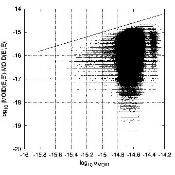
In Fig. 2 we compare the quadrature sum of the reported MOID uncertainties, , with the difference that can be deemed as an empiric estimate of the actual MOID error. We may conclude that our algorithm provides rather safe and realistic assessment of numeric errors, intentionally a bit pessimistic. We did not met a case with the empiric error exceeding the predicted uncertainty.


From Fig. 3 one can see that we spend, in average, about Newtonian iterations per each root. One way how we may further increse the speed of computation is to reduce this number. However, this number is already quite small, so there is no much room to significantly reduce it. On the refining stage the algorithm usually performs just one or two 2D Newtonian iterations in the plane . The fraction of occurences when three or more refining iterations are made is very small and further decreases quickly. The maximum number of refining iterations made in this test was .
| Hardware | double arithmetic | long double arithmetic | ||
|---|---|---|---|---|
| distlink | Gronchi code | distlink | Gronchi code | |
| (fast alg.) | (fast alg.) | |||
| Intel Core i7 | s | s | s | NA |
| Supermicro & Xeon | s | s | s | NA |
| AMD FX | s | s | s | NA |
In Table 1, we present our performance benchmarks for this test application. They were done for the following hardware: (i) Intel Core i7-6700K at GHz, (ii) Supermicro server with Intel Xeon CPU E5-2630 at GHz, and (iii) AMD 990FX chipset with AMD FX-9590 CPU at GHz. The second configuration is rather similar to one of those used by Hedo et al. 2018.
We used either 80-bit long double floating-point arithmetic or the 64-bit double one, and requested the desired accuracy of : or , respectively. We did not use , because in the double case many CPUs hiddenly perform much of the local computation in long double precision instead of the requested double. Newtonian iterations are then continued to this undesiredly increased level of precision, if , thus introducing an unnecessary minor slowdown. The least required accuracy was set to in all of the tests.
All the code was compiled with GCC (either g++ or gfortran) and optimized for the local CPU architecture (-O3 -march=native -mfpmath=sse). The Gronchi primary computing subroutine compute_critical_points_shift() was called from our C++ program natively, i.e. without any intermediary file IO wrapping that would be necessary if we used the main program CP_comp.x from the Gronchi package.
To accurately measure the time spent purely inside just the MOID computation, and not on the file IO or other algorithmic decorations around it, we always performed three independent runs on the test catalog: (i) an ‘empty’ run without any calls to any MOID algorithm, only iteration over the catalog; (ii) computation of all MOIDs using the algorithm of this paper, without writing results to a file; (iii) same for the Gronchi algorithm. The time differences (ii)-(i) or (iii)-(i) gave us the CPU time spent only inside the MOID computation. We never included the CPU time spent in the kernel mode. We assume this system time likely refers to some memory pages manipulation or other similar CPU activity that appears when the program iteratively accesses data from a big catalog. In any case, this system time would be just a minor addition to the result ( per cent at most).
The reader may notice that the hardware can generate huge performance differences, not necessarily owing to just the CPU frequency. Moreover, even the performance on the same AMD machine differs drastically between the double and long double tests. This puzzling difference appears mainly due to slow 80-bit floating-point arithmetic on AMD, not because of e.g. different number of Newtonian iterations per root (which appeared almost the same in all our tests, – iterations per root).
We conclude that our algorithm looks quite competitive and probably even outperforming the benchmarks obtained by Hedo et al. 2018 for their set of tested algorithms (– s per orbit pair on a Supermicro/Xeon hardware). They used double precision rather than long double one.
Therefore, our algorithm possibly pretends to be the fastest one available to date, or at least it belongs to the family of the fastest ones. In the majority of cases it yields considerably more accurate and reliable results, usually close to the machine precision, and its accuracy may seriously degrade only in extraordinary rare nearly degenerate cases, which are objectively hard to process.
6 Additional tools
Our main algorithm based on determining the roots of is fast but might become vulnerable in the rare cases of lost roots. Whenever it signals a warning, alternative algorithms should be used, trading computing speed for better numeric resistance with respect to degeneracies.
In addition to the basic 0D method based on root-finding, our library implements a “fallback” algorithm of the 1D type, based on the brute force-like minimization of . This method is numerically reliable thanks to its simplicity, and its slow speed is not a big disadvantage, because it needs to be run only if the basic fast method failed. In our benchmarking test it appeared times or times slower than our fast algorithm or the Gronchi code, respectively. But this is likely sensitive to its input parameters.
First of all, the algorithm scans only a restricted range in the variable, discarding the values where the MOID cannot be attained. The requied range is determined as follows. Using e.g. formulae from (Kholshevnikov and Vassiliev 1999a), compute the minimum internodal distance . Since MOID is usually attained near the orbital nodes, this quantity and its corresponding orbital positions already provide rather good approximation to the MOID. Then consider two planes parallel to the orbit , and separated from it by . We need to scan only those pieces of orbit that lie between these planes, i.e. lie within band from the plane. The points on outside of this set are necessarily more distant from than , so the MOID cannot be attained there. This trick often reduces the range dramatically. This optimization was inspired by the discussion given in (Hedo et al. 2018). The detailed formulae for the reduced range of are given in A.
Moreover, this algorithm automatically selects the optimal orbits order or to have a smaller angular range to scan. In the case if the cumulative ranges appear equal (e.g. if we occasionally have the full-circle in both cases) then the user-supplied order is preserved.
The efficiency of this approach is demonstrated in Fig. 4, where we plot the distribution density for the total range length obtained, as computed for our test case of asteroid pairs. The fraction of the cases in which this range could not be reduced at all (remained at ) is only , and in the majority of occurences it could be reduced to something well below rad. The efficiency of the reduction increases if MOID is small. Then the total scan range may be reduced to just a few degrees.

The minimization of is based on subsequent sectioning of the initial angular range for . The user can set an arbitrary sequence of integer numbers that define how many segments are considered at different stages. The initial angular range is partitioned into equal segments separated by the equidistant nodes , and the node with a minimum is determined. We note that the input parameter is always interpreted as if it corresponded to the entire range, even if the actual scan range is reduced as described above. The segment length on the first step is normally set to regardless of the scan range, unless this scan range is itself smaller than . On the second stage, the segment surrounding the minimum is considered. It is sectioned into equal segments, and the node corresponding to the minimum is determined again. On the third stage, the segment is sectioned into smaller segments, and so on. On the th stage, the length of the segment between subsequent nodes is reduced by the factor , so only are meaningful. Starting from the stage number , the segments are always partitioned into subsegments, until the global minimum of is located with a desired accuracy in and . It is recommended to set large enough, e.g. , in order to sample the objective function with its potentially intricate variations densely enough, whereas the last can be set to , meaning the bisection.
We notice that this method was not designed for a standalone use. It was not even supposed to be either more reliable or more accurate in general than our primary fast method. It was supposed to provide just yet another alternative in rare special cases when the primary method did not appear convincingly reliable. Its practical reliability depends on the input parameters very much: too small may lead to frequent loosing of local minima in , if they are narrow. Hence we may miss the correct global minimum sometimes. But this effect can be always suppressed by selecting a larger . In our tests, with this algorithm generated one wrong MOID per trials, so it is not recommended for a general sole use. This could be improved by implementing an adaptive sampling in the variable, e.g. depending on the derivative , but we did not plan to go that far with this method. We note that narrow local minima of are, informally speaking, in some sense antagonistic to almost-multiple critical points, so this fallback algorithm is vulnerable to rather different conditions than our primary fast method. Therefore it can serve as a good complement to the latter.
Also, we include in the library several fast tools that may appear useful whenever we need to actually compute the MOID only for those object that are close to an orbital intersection. These tools may help to eliminate most of the orbit pairs from the processing. The first one represents an obvious pericenter–apocenter test: , and . If any of these quantities appeared positive and above some upper threshold then surely , and one may immediately discard such orbital pair from the detailed analysis.
Our library also includes functions for computing the so-called linking coefficients introduced by Kholshevnikov and Vassiliev 1999a. The linking coefficients are functions of two orbits that have the dimension of squared distance, like , and they are invariable with respect to rotations in . Kholshevnikov and Vassiliev 1999a introduced three linking coefficients that should be selected depending on whether the orbits are (nearly) coplanar or not. See all the necessary formulae and discussion in that work.
For our goals it might be important that at least one of these linking coefficients, , can be used as an upper limit on the MOID. It represents a signed product of two internodal distances from (51), so the squared MOID can never be larger than . This allows us to limit the MOID from another side, contrary to the pericenter-apocenter test. Moreover, based on we introduce yet another linking coefficient defined as
| (45) |
This modified provides even tighter upper limit on the squared MOID, but still preserves the sign that indicates the orbital linkage in the same way as did.
It is important for us that all linking coefficients are computed very quickly in comparison to any MOID algorithm, because they are expressed by simple elementary formulae.
The linking coefficients were named so because their original purpose was to indicate whether two orbits are topologically linked like two rings in a chain, or not. The intermediate case between these two is an intersection, when the linking coefficient vanishes together with the MOID. Therefore, these indicators can be potentially used as computationally cheap surrogates of the MOID. But in addition to measuring the closeness of two orbits to an intersection, linking coefficients carry information about their topological configuration. Also, these quantities can be used to track the time evolution of the mutual topology of perturbed non-Keplerian orbits, for example to locate the moment of their intersection without computing the MOID.
7 Further development and plans
Yet another possible way to extend our library is to implement the method by Baluyev and Kholshevnikov 2005 for computing the MOID between general confocal unperturbed orbits, including hyperbolic and parabolic ones. This task can be also reduced to finding real roots of a polynomial similar to .
In a future work we plan to provide statistical results of applying this algorithm to the Main Belt asteroids, also including the comparison of the MOID with linking coefficients and other indicators of orbital closeness.
Acknowledgements
This work was supported by the Russian Science Foundation grant no. 18-12-00050. We express gratitude to the anonymous reviewers for the fruitful comments and useful suggestions on the manuscript.
Appendix A Reducing the scan range for the eccentric anomaly
Let us introduce , which is a unit vector orthogonal to the orbital plane of . The vectors , , form an orthonormal basis in . Then from (22) let us compute the dot-product
| (46) |
which represents a projection of the distance vector on the basis vector . Note that the dot-product is always zero. Now, we need this distance projection to be within from zero, because otherwise the absolute distance can be only larger than . This yields two inequality constraints
| (47) |
implying an elementary trigonometric equation that can be solved via arcsines.
The final set of computing formulae can be expressed as follows. Let us introduce the vector
| (48) |
which is directed to the ascending node of assuming reference . The angle is the mutual inclination between the orbits. Then determine the angle from
| (49) |
It represents the true anomaly on , where that ascending node is located. Basically, is the angle between and , counted positive in the direction of . The location on the other orbit can be determined in a similar way. Explicit formula for the scalar product is given in (Kholshevnikov and Vassiliev 1999a) via orbital elements, though we prefer to multiply the vectors directly, using the following expression for :
After that let us compute
| (51) |
where and are orbital parameters, .
Now, the inequalities (47) may be simplified if we decompose the vectors and in the basis :
| (52) |
Writing down the orthogonality condition between and and the norm of in these coordinates, we have
| (53) |
Therefore, we may set and in (47), and the sign choice is not important here.
In general, we have three types of solution for .
- 1.
If and then we have two small segments for near the nodes, defined as and ;
- 2.
If and then we have the entire circular range for .
- 3.
If then there is just one big segment for that covers angles roughly from one node to another, defined as either , if , or , if ;
In practice, the first type of occurence is the most frequent one, so the speed improvement is dramatic. Notice that for (coplanar orbits) the angle formally becomes undefined, but this is not important because then and we just obtain the full-circle range for . So the degenerate case is not a big numeric issue in practice.
References
- Armellin et al. (2010) Armellin, R., di Lizia, P., Berz, M., Makino, K., 2010. Computing the critical points of the distance function between two Keplerian orbits via rigorous global optimization. Celest. Mech. Dyn. Astron. 107, 377–395.
- Baluyev and Kholshevnikov (2005) Baluyev, R.V., Kholshevnikov, K.V., 2005. Distance between two arbitrary unperturbed orbits. Celest. Mech. Dyn. Astron. 91, 287–300.
- Dybczyński et al. (1986) Dybczyński, P.A., Jopek, T.J., Serafin, R.A., 1986. On the minimum distance between two Keplerian orbits with a common focus. Celest. Mech. 38, 345–356.
- Gronchi (2002) Gronchi, G.F., 2002. On the stationary points of the squared distance between two ellipses with a common focus. SIAM J. Sci. Comput. 24, 61–80.
- Gronchi (2005) Gronchi, G.F., 2005. An algebraic method to compute the critical points of the distance function between two Keplerian orbits. Celest. Mech. Dyn. Astron. 93, 295–329.
- Hedo et al. (2018) Hedo, J.M., Ruíz, M., Peláez, J., 2018. On the minimum orbital intersection distance computation: a new effective method. MNRAS 479, 3288–3299.
- Kholshevnikov and Vassiliev (1999a) Kholshevnikov, K., Vassiliev, N., 1999a. On linking coefficient of two Keplerian orbits. Celest. Mech. Dyn. Astron. 75, 67–74.
- Kholshevnikov and Vassiliev (1999b) Kholshevnikov, K., Vassiliev, N., 1999b. On the distance function between two Keplerian elliptic orbits. Celest. Mech. Dyn. Astron. 75, 75–83.
- Sitarski (1968) Sitarski, G., 1968. Approaches of the parabolic comets to the outer planets. Acta Astronomica 18, 171–195.