跳到论文正文
W Papers独立论文阅读器 arXiv:1811.06239 论文正文 计算阅读时间 · 0%
引用这篇论文根据当前论文元数据生成,正式投稿前建议核对。


License: arXiv.org perpetual non-exclusive license
arXiv:1811.06239v1 [math.NA] 15 Nov 2018

Error and stability analysis of an anisotropic phase-field model for binary-fluid mixtures in the presence of magnetic-field

A. Rasheed Thanks: Department of Mathematics, Lahore University of Management Sciences, Opposite Sector U, DHA,Lahore Cantt 54792, Pakistan, amer.rasheed@lums.edu.pk,    A. Belmiloudi Thanks: Mathematics Research Institute of Rennes (IRMAR), European University of Brittany, INSA, 20 Av. Buttes de Coesmes, CS70839, 35708 Rennes Cedex7, France, aziz.belmiloudi@math.cnrs.fr
Abstract

In this article, we study the error and stability of the proposed numerical scheme in order to solve a two dimensional anisotropic phase-field model with convection and externally applied magnetic field in an isothermal solidification of binary alloys. The proposed numerical scheme is based on mixed finite element method satisfying the CFL condition. A particular application with real physical parameters of Nickel-Copper(Ni-Cu) is considered in order to validate the numerical scheme employed. The results of stability and error analysis substantiates complete accordance with the postulated theoretical error estimates which demonstrates the efficiency of the presented method.

keyword Phase field methods; Stability and error analysis; binary alloys; magnetic-field.

1 Introduction

The quality of the final solidified metal is dependent on the dendrite structure evolution during the process of solidification of metals. In order to ameliorate the quality of the solidified materials, it is important to understand and render control over dendritic structure formation during the process of solidification of alloys. During the past decade, the scientists have investigated a great deal of experimental and theoretical studies to explore the microstructure of dendrites during the process of solidification of alloys. Phase field method has been widely used by researchers in order to simulate and study the structure and formation of dendrites (see for instance [1, 2, 3, 6, 10, 15, 16, 17, 27, 29, 30, 31]) and the references therein. Unfortunately, the presented models donot render control on dendritic evolution and micro-segregation. Moreover, some experimental observations show that the control on dendrite growth can be achieved in the during the solidification process by applying electric and magnetic fields externally, see for example [14, 24] and the references therein. For similar other applications wherin authors have discussed the effect of magnetic field on the metals and alloys, refer to the studies, e.g., for the semi-conductor flow in the melt crystal evolution, [7], for the MHD flows [12], [11], [32], [9] and for the processes of dendritic solidification, [23], [24], [25] and the references therein.

In view of aforementioned facts, Rasheed and Belmiloudi in [20] (see also [18, 19, 22]) has presented a phase-field model which incorporates melt flow and magnetic field. Initially, the model of Warren-Boettinger [31] is considered and then, among other, Navier Stokes equations, the phase-field and solute equations with a magnetic field applied externally on the domain. The newly developed phase-field model consists three systems, the magnetohydrodynamic system which describes the melt convection by using incompressible Navier-Stokes equations together with the Lorentz force and boussinesq approximations, the phase-field system which represents the phase change and the concentration system describing the concentration change in dendrites during solidification process. The phase field and concentration equations are of convection diffusion type systems. We refer the reader to [20] for more detailed description of the model.

The existence and uniqueness of the solutions of the derived model is presented in the article [20]. In order to perform realistic physical simulations it is indispensable to develop a stable and convergent numerical scheme. This article is devoted to present a numerical approximation scheme using mixed finite-elements and numerical stability and error analysis for Rasheed and Belmiloudi model [RasheedBelmiloudi] for the anisotropic case. Some numerical results in the isotropic case are presented in the article [21].

The paper has been organized as follows. In section 2 we recall the mathematical model briefly and its weak formulation in section 3. Section 4 is describes the discrete variational formulation, in the context of a mixed finite element method. The numerical stability and error analysis are presented and validated by numerical experiments in section 5.

2 Mathematical formulation

Initially a region Ω\Omega is assumed to be occupied by a binary alloy containing two pure elements, the solute B (e.g., Cu) and the solvent A (e.g., Ni), which is electrically conducting incompressible fluid. To construct a numerical scheme and study its numerical stability and error, we recall the model for dendritic solidification given by [20]. Let 𝐮\mathbf{u}, pp, ψ\psi, cc and 𝐁\mathbf{B} represent the velocity vector, pressure, phase-field variable, relative concentration and externally magnetic field respectively. Wwe have the following system

{ρ0(∂t𝐮+(𝐮⋅∇)𝐮)=−∇p+μΔ𝐮+𝓐1(ψ,c)+b(ψ)((𝐮×𝐁)×𝐁)on𝒬,div​𝐮=0on𝒬,∂tψ+(𝐮⋅∇)ψ=div(𝒜g(∇ψ)∇ψ)−𝒜2(ψ,c)on𝒬,∂tc+(𝐮⋅∇)c=div(D(ψ)∇c+𝒜3(ψ,c)∇ψ)on𝒬,subject to the initial conditions(𝐮,ψ,c)​(t=0)=(𝐮0,ψ0,c0)onΩ,and the boundary conditions𝐮=0,𝒜g(∇ψ)∇ψ⋅𝐧=0,(D(ψ)∇c+𝒜3(ψ,c)∇ψ)⋅𝐧=0onΣ,\hskip-8.5359pt\begin{cases}\displaystyle\rho_{0}\big(\partial_{t}\mathbf{u}+(\mathbf{u}\cdot\nabla)\mathbf{u}\big)=-\nabla p+\mu\Delta\mathbf{u}+\boldsymbol{\mathcal{A}}_{1}(\psi,c)+b(\psi)\big(\left(\mathbf{u}\times\mathbf{B}\big)\times\mathbf{B}\right)&\text{on}\penalty\ \penalty\ {\cal Q},\\ \displaystyle\rm{div}\mathbf{u}=0&\text{on}\penalty\ \penalty\ {\cal Q},\\ \displaystyle\partial_{t}\psi+(\mathbf{u}\cdot\nabla)\psi=\rm{div}\left(\mathcal{A}_{g}(\nabla\psi)\nabla\psi\right)-\mathcal{A}_{2}(\psi,c)&\text{on}\penalty\ \penalty\ {\cal Q},\\ \displaystyle\partial_{t}c+(\mathbf{u}\cdot\nabla)c=\rm{div}\left(D(\psi)\nabla c+\mathcal{A}_{3}(\psi,c)\nabla\psi\right)&\text{on}\penalty\ \penalty\ {\cal Q},\\ \text{subject to the initial conditions}\\ \left(\mathbf{u},\psi,c\right)(t=0)=\left(\mathbf{u}_{0},\psi_{0},c_{0}\right)&\text{on}\penalty\ \penalty\ \Omega,\\ \text{and the boundary conditions}\\ \mathbf{u}=0,\quad\mathcal{A}_{g}(\nabla\psi)\nabla\psi\cdot\mathbf{n}=0,\quad(D(\psi)\nabla c+\mathcal{A}_{3}(\psi,c)\nabla\psi)\cdot\mathbf{n}=0&\text{on}\penalty\ \penalty\ \Sigma,\end{cases} (2.1)

where Ω⊂ℜ2\Omega\subset\Re^{2} is a Lipschitz and sufficiently smooth open solidification domain with polygonal boundary ∂Ω\partial\Omega, TT is the final time of the solidification process, 𝒬=Ω×(0,T){\cal Q}=\Omega\times\left(0,T\right), Σ=∂Ω×(0,T)\Sigma=\partial\Omega\times\left(0,T\right), ρ0=ρ0(A)+ρ0(B)2\rho_{0}=\frac{\rho_{0}^{(A)}+\rho_{0}^{(B)}}{2} and μ=μ(A)+μ(B)2\mu=\frac{\mu^{(A)}+\mu^{(B)}}{2} are the average density and viscosity, D⁡(ψ)D(\psi) is the diffusion coefficient and 𝐧\mathbf{n} is the unit outward normal to ∂Ω\partial\Omega. The anisotropy matrix 𝒜g\mathcal{A}_{g} is defined by

𝒜g​(∇ψ)=Mψ​(ηγ2​(θ)−ηγ​(θ)​ηγ′​(θ)ηγ​(θ)​ηγ′​(θ)ηγ2​(θ))\mathcal{A}_{g}(\nabla\psi)=M_{\psi}\begin{pmatrix}\eta^{2}_{\gamma}(\theta)&-\eta_{\gamma}(\theta)\eta^{\prime}_{\gamma}(\theta)\\ \eta_{\gamma}(\theta)\eta^{\prime}_{\gamma}(\theta)&\eta^{2}_{\gamma}(\theta)\end{pmatrix}

where Mψ>0M_{\psi}>0 and ηγ\eta_{\gamma} is the anisotropy function defined as [31]

ηγ=ϵ0​(1+γ​cos⁡(k​θ)),\eta_{\gamma}=\epsilon_{0}(1+\gamma\cos(k\theta)), (2.2)

γ≥0\gamma\geq 0 is the anisotropic amplitude, the integer k>1k>1 corresponds to the number of branching directions, ϵ0\epsilon_{0} is a constant and θ\theta (the angle between the xx-axis and ∇ψ\nabla\psi)

θ=arctan⁡(ψyψx),\theta=\arctan\left(\frac{\psi_{y}}{\psi_{x}}\right), (2.3)

where xx and yy are subscripts used to represent the partial derivatives with respect to spatial coordinates, that is ψx=∂ψ/∂x\psi_{x}=\partial\psi/\partial x and ψy=∂ψ/∂y\psi_{y}=\partial\psi/\partial y. For low to moderate accuracy, γ>0\gamma>0 is selected so that the condition ηγ​(θ)+d2​ηγd​θ2​(θ)>0\displaystyle\eta_{\gamma}(\theta)+\frac{d^{2}\eta_{\gamma}}{d\theta^{2}}(\theta)>0 is valid for all θ\theta. For k=4k=4 (fourfold anisotropy) which is a case of physical appearance, the previous condition is valid if γ<115≈0,6667\gamma<\frac{1}{15}\approx 0,6667. The operators 𝓐𝟏\boldsymbol{\mathcal{A}_{1}}, 𝒜2\mathcal{A}_{2} and 𝒜3\mathcal{A}_{3} are defined by

𝓐𝟏(ψ,c)=βca1(ψ)c𝐆+ζ𝐟(ψ),𝒜2(ψ,c)=Mψ(λ1​(c)δ2g′(ψ)+λ2​(c)δp¯′(ψ)),𝒜3​(ψ,c)=α0​D​(ψ)​c​(1−c)​(λ1′​(c)δ​g′​(ψ)−λ2′​(c)​p¯′​(ψ)),\begin{array}[]{lcr}\boldsymbol{\mathcal{A}_{1}}(\psi,c)=\beta_{c}a_{1}(\psi)c\mathbf{G}+\zeta{\bf f}(\psi),\quad\displaystyle\mathcal{A}_{2}(\psi,c)=M_{\psi}(\frac{\lambda_{1}(c)}{\delta^{2}}g^{\prime}(\psi)+\frac{\lambda_{2}(c)}{\delta}\bar{p}^{\prime}(\psi)),\\ \displaystyle\mathcal{A}_{3}(\psi,c)=\alpha_{0}D(\psi)c(1-c)\left(\frac{\lambda_{1}^{\prime}(c)}{\delta}g^{\prime}(\psi)-\lambda_{2}^{\prime}(c)\bar{p}^{\prime}(\psi)\right),\\ \end{array} (2.4)

For a detailed description and derivation of the mathematical model, the reader is referred to [20].

3 Weak formulation

The inner product and norm in L2​(Ω)L^{2}(\Omega) are defined respectively by (.,.)(.,.) and ∣.∣\mid.\mid and

𝒲=(H01(Ω))2={v∈(H1(Ω))2|v=0on∂Ω},𝒲d={v∈𝒲|div(v)=0},ℳ=H1(Ω),ℋ={q∈L2(Ω)|∫Ωqdx=0},\displaystyle\begin{array}[]{lll}&\displaystyle{\cal{W}}=(H_{0}^{1}(\Omega))^{2}=\left\{\textbf{v}\in\ \left(H^{1}(\Omega)\right)^{2}\ |\ \textbf{v}=0\ \mbox{on}\ \partial\Omega\right\},\ \ \ \displaystyle{\cal{W}}_{d}=\left\{\textbf{v}\in\ {\cal{W}}\ |\ \rm{div}(\textbf{v})=0\ \right\},\\ &\displaystyle{\cal{M}}=H^{1}(\Omega),\ \ \ \displaystyle{\cal{H}}=\left\{q\in L^{2}(\Omega)\ \left|\right.\int_{\Omega}qd\textbf{x}=0\right\},\end{array}

where 𝒲{\cal{W}} is equipped with the norm ∥∇.∥\parallel\nabla.\parallel. The scalar product and norm in ℋ{\cal{H}} are denoted by the usual L2​(Ω)L^{2}(\Omega) inner product and its norm (.,.)(.,.) and ∣.∣\mid.\mid, respectively.

Remark 3.1

: In order to assure that the pressure is unique, we impose the condition ∫Ωq​𝑑x=0\displaystyle\int_{\Omega}qd\textbf{x}=0 on the pressure which is defined within a class of equivalence, regardless of a time-dependent function. We may impose also other conditions on the pressure, in accordance on its regularity, e.g., the pressure is constant on part of the boundary, etc.

The bilinear and trilinear forms are defined as follows (for all (𝐮,𝐯,𝐰)∈(𝒲)3(\mathbf{u},\mathbf{v},\mathbf{w})\in({\cal{W}})^{3}, p∈ℋp\in{\cal{H}}, (c,z)∈(ℳ)2(c,z)\in({\cal{M}})^{2} and (ϕ,ψ)∈(ℳ)2(\phi,\psi)\in({\cal{M}})^{2}):

au(𝐮,𝐯)=μ∫Ω∇𝐮⋅∇𝐯d𝐱,cp(u,p)=−(div(u),p),bu(𝐮,𝐯,𝐰)=ρ0∑i,j=12∫Ωui(∂ivj)wjd𝐱,bc(𝐮,c,z)=∑i=12∫Ωui(∂ic)zd𝐱,bψ(𝐮,ψ,ϕ)=∑i=12∫Ωui(∂iψ)ϕd𝐱.\displaystyle\begin{array}[]{lll}&\displaystyle a_{u}(\mathbf{u},\mathbf{v})=\mu\int_{\Omega}\nabla\mathbf{u}\cdot\nabla\mathbf{v}d\mathbf{x},\ \ c_{p}\left(\textbf{u},p\right)=-\left(\rm{div}(\textbf{u}),p\right),\ \ b_{u}(\mathbf{u},\mathbf{v},\mathbf{w})=\rho_{0}\sum_{i,j=1}^{2}\int_{\Omega}u_{i}(\partial_{i}v_{j})w_{j}d\mathbf{x},\\ &\displaystyle b_{c}(\mathbf{u},c,z)=\sum_{i=1}^{2}\int_{\Omega}u_{i}(\partial_{i}c)zd\mathbf{x},\ \ b_{\psi}(\mathbf{u},\psi,\phi)=\sum_{i=1}^{2}\int_{\Omega}u_{i}(\partial_{i}\psi)\phi d\mathbf{x}.\end{array}

Moreover, if div⁡(𝐮)=0\rm{div}(\mathbf{u})=0, the trilinear forms satisfy the classical relations given in the following Lemma (see e.g. [5, 28]):

Lemma 3.1

The trilinear forms bu,bψ,bcb_{u},b_{\psi},b_{c} have the following properties

  • (i)

    For all u∈𝒲d,v∈𝒲\textbf{u}\in{\cal{W}}_{d},\ \textbf{v}\in{\cal{W}} and ψ,c∈ℳ\psi,c\in{\cal{M}}

    bu​(u,v,v)=0,bψ​(u,ψ,ψ)=0,bc​(u,c,c)=0.\displaystyle b_{u}(\textbf{u},\textbf{v},\textbf{v})=0,\ \ b_{\psi}(\textbf{u},\psi,\psi)=0,\ \ b_{c}(\textbf{u},c,c)=0.
  • (ii)

    For all u∈𝒲d,v,w∈𝒲\textbf{u}\in{\cal{W}}_{d},\ \textbf{v},\textbf{w}\in{\cal{W}} and ψ,ϕ,c,z∈ℳ\psi,\phi,c,z\in{\cal{M}}

    bu​(u,v,w)=−bu​(u,w,v),bψ​(u,ψ,ϕ)=−bψ​(u,ϕ,ψ),bc​(u,c,z)=−bc​(u,z,c).\displaystyle b_{u}(\textbf{u},\textbf{v},\textbf{w})=-b_{u}(\textbf{u},\textbf{w},\textbf{v}),\ \ b_{\psi}(\textbf{u},\psi,\phi)=-b_{\psi}(\textbf{u},\phi,\psi),\ \ b_{c}(\textbf{u},c,z)=-b_{c}(\textbf{u},z,c).

In order to obtain the weak formulations of the underlying model we multiply the first and second equations of (2.1) by v∈𝒲\textbf{v}\in{\cal{W}}, third equation of (2.1) by ϕ∈ℳ\phi\in{\cal{M}} and last equation of (2.1) by z∈ℳz\in{\cal{M}}. Further we integrate the results over Ω\Omega and then using Green’s formulas and boundary conditions, we obtain the following weak formulation of the problem (2.1) (wherein we added an artificial source term Fu\textbf{F}_{u}, FψF_{\psi} and FcF_{c} in each equation of the model for fabricating exact solutions to perform the convergence and stability of the numerical scheme): Find (u,p,ψ,c)∈𝒲×ℋ×ℳ×ℳ(\textbf{u},p,\psi,c)\in\cal{W}\times\cal{H}\times\displaystyle{\cal{M}}\times\displaystyle{\cal{M}} such that ∀(v,q,φ,z)∈𝒲×ℋ×ℳ×ℳ\forall\ (\textbf{v},q,\varphi,z)\in\cal{W}\times\cal{H}\times\displaystyle{\cal{M}}\times\displaystyle{\cal{M}}

{ρ0​(∂tu,v)+au​(u,v)+bu​(u,u,v)+cp​(v,p)−(𝓐1​(ψ,c),v)−(b⁡(ψ)​((u×B)×B),v)=(Fu,v),−cp​(u,q)=0,(∂tψ,φ)+bψ(u,ψ,φ)+(𝒜g(∇ψ)∇ψ,∇φ)+(𝒜2(ψ,c),φ)=(Fψ,φ),(∂tc,z)+bc(u,c,z)+(D(ψ)∇c,∇z)+(𝒜3(ψ,c)∇ψ,∇z)=(Fc,z),(u,ψ,c)​(t=0)=(u0,ψ0,c0).\hskip-8.5359pt\begin{cases}&\displaystyle\rho_{0}\left(\partial_{t}\textbf{u},\textbf{v}\right)+a_{u}(\textbf{u},\textbf{v})+b_{u}(\textbf{u},\textbf{u},\textbf{v})+c_{p}\left(\textbf{v},p\right)-\left(\boldsymbol{\mathcal{A}}_{1}(\psi,c),\textbf{v}\right)\\ &\displaystyle\hskip 85.35826pt-\left(b(\psi)((\textbf{u}\times\textbf{B})\times\textbf{B}),\textbf{v}\right)=\left(\textbf{F}_{u},\textbf{v}\right),\\ &\displaystyle-c_{p}\left(\textbf{u},q\right)=0,\\ &\displaystyle\left(\partial_{t}\psi,\varphi\right)+b_{\psi}(\textbf{u},\psi,\varphi)+(\mathcal{A}_{g}(\nabla\psi)\nabla\psi,\nabla\varphi)+\left(\mathcal{A}_{2}(\psi,c),\varphi\right)=\left(F_{\psi},\varphi\right),\\ &\displaystyle\left(\partial_{t}c,z\right)+b_{c}(\textbf{u},c,z)+\left(D(\psi)\nabla c,\nabla z\right)\displaystyle+\left(\mathcal{A}_{3}(\psi,c)\nabla\psi,\nabla z\right)=\left(F_{c},z\right),\\ &\displaystyle\left(\textbf{u},\psi,c\right)(t=0)=\left(\textbf{u}_{0},\psi_{0},c_{0}\right).\end{cases} (3.3)

4 Discrete weak formulation and finite element discretization

Let 𝒯h{\cal T}_{h} be a family of triangulations which discretize the domain Ω¯\overline{\Omega} with maximum mesh spacing parameter 0<h=max℧∈𝒯h⁡d​i​a​m​(Ω)<h0<10<h=\max_{\mho\in{\cal T}_{h}}diam(\Omega)<h_{0}<1. To develop the Galerkin approximation of (3.3), we consider the ℙl\mathbb{P}_{l}, ℙl−1\mathbb{P}_{l-1} and ℙl\mathbb{P}_{l} finite element subspaces 𝒲h{\cal W}_{h}, ℋh{\cal H}_{h} and ℳh{\cal M}_{h} of 𝒲\cal{W}, ℋ\cal{H} and ℳ\cal{M} respectively over the partition 𝒯h{\cal T}_{h}, where the polynomials ℙl\mathbb{P}_{l} is the space of polynomials of degree at most ll. Furthermore, in order to derive theoretical error estimates of the PDEs like 2.1, we impose the following assumptions (see [4, 26])

  1. (C1)

    ∃c1>0\exists\ c_{1}>0, such that ∀X=(u,ψ,c)∈(Hr+1​(Ω))4∩(𝒲×ℳ2)\forall\textbf{X}=(\textbf{u},\psi,c)\in\left(H^{r+1}(\Omega)\right)^{4}\cap\left({\cal W}\times{\cal M}^{2}\right) and ∀r∈[1,l]\forall r\in\left[1,l\right]

    infXh∈𝒲h×ℳh2‖X−Xh‖≤c1​hr​‖X‖Hr+1​(Ω).\displaystyle\inf_{\textbf{X}_{h}\in{\cal W}_{h}\times{\cal M}^{2}_{h}}\left\|\textbf{X}-\textbf{X}_{h}\right\|\ \leq\ c_{1}h^{r}\left\|\textbf{X}\right\|_{H^{r+1}(\Omega)}.
  2. (C2)

    ∃c2>0\exists\ c_{2}>0, such that ∀q∈Hr​(Ω)∩ℋ\forall\ q\in H^{r}(\Omega)\cap{\cal H} and ∀r∈[1,l]\forall\ r\in\left[1,l\right]

    infqh∈ℋh‖q−qh‖≤c2​hr​‖q‖Hr​(Ω).\displaystyle\inf_{q_{h}\in{\cal H}_{h}}\left\|q-q_{h}\right\|\ \leq\ c_{2}h^{r}\left\|q\right\|_{H^{r}(\Omega)}.
  3. (C3)

    ∃c3>0\exists\ c_{3}>0 such that (Inf-Sup condition)

    infqh∈ℋhsupvh∈𝒲hcp​(vh,qh)‖vh‖​|qh|≥c3.\displaystyle\inf_{q_{h}\in{\cal H}_{h}}\sup_{\textbf{v}_{h}\in{\cal W}_{h}}\frac{c_{p}(\textbf{v}_{h},q_{h})}{\left\|\textbf{v}_{h}\right\|\left|q_{h}\right|}\ \geq\ c_{3}.
  4. (C4)

    Let X0=(u0,ψ0,c0)∈(Hr+1​(Ω))4\textbf{X}_{0}=(\textbf{u}_{0},\psi_{0},c_{0})\in\left(H^{r+1}(\Omega)\right)^{4} with r∈[1,l]r\in[1,l], then

    h⁡‖X0−X0​h‖+|X0−X0​h|≤c4​hr+1,\displaystyle h\left\|\textbf{X}_{0}-\textbf{X}_{0h}\right\|+\left|\textbf{X}_{0}-\textbf{X}_{0h}\right|\ \leq\ c_{4}h^{r+1},

    where X0​h=(u0​h,ψ0​h,c0​h)∈𝒲h×ℳh2\textbf{X}_{0h}=(\textbf{u}_{0h},\psi_{0h},c_{0h})\in{\cal W}_{h}\times{\cal M}^{2}_{h} is the approximation of X0\textbf{X}_{0}.

  5. (C5)

    For all integers 𝔪,𝔭,𝔮\mathfrak{m},\mathfrak{p},\mathfrak{q} and 𝔨\mathfrak{k} with 0<𝔭,𝔮≤∞0<\mathfrak{p},\mathfrak{q}\leq\infty and ∀K∈𝒯h\forall\ K\in{\cal T}_{h}, we have

    ‖Xh‖W𝔪,𝔮​(K)≤c4​hn/𝔮−n/𝔭+𝔨−𝔪​‖Xh‖W𝔨,𝔭​(K),∀Xh∈𝒲h×ℳh2,\displaystyle\left\|\textbf{X}_{h}\right\|_{W^{\mathfrak{m},\mathfrak{q}}(K)}\ \leq\ c_{4}\ h^{n/\mathfrak{q}-n/\mathfrak{p}+\mathfrak{k}-\mathfrak{m}}\ \left\|\textbf{X}_{h}\right\|_{W^{\mathfrak{k},\mathfrak{p}}(K)},\ \ \ \forall\ \textbf{X}_{h}\in{\cal W}_{h}\times{\cal M}^{2}_{h},
    ‖Xh‖W𝔪,𝔮​(Ω)≤c4​hn/𝔮−n/𝔭+𝔨−𝔪​‖Xh‖W𝔨,𝔭​(Ω),∀Xh∈𝒲h×ℳh2.\displaystyle\left\|\textbf{X}_{h}\right\|_{W^{\mathfrak{m},\mathfrak{q}}(\Omega)}\ \leq\ c_{4}\ h^{n/\mathfrak{q}-n/\mathfrak{p}+\mathfrak{k}-\mathfrak{m}}\ \left\|\textbf{X}_{h}\right\|_{W^{\mathfrak{k},\mathfrak{p}}(\Omega)},\ \ \ \forall\ \textbf{X}_{h}\in{\cal W}_{h}\times{\cal M}^{2}_{h}.

The space and time discretization of the problem (3.3) i.e. the discrete weak formulation of the problem (2.1) can now be easily defined. We shall describe in detail the numerical scheme and present the space discretization and the general form of the differential-algebraic systems for (3.3). Further we present the time discretization of the problem briefly. The discrete weak formulation is presented as follows: Find (uh,ph,ψh,ch)∈𝒲h×ℋh×ℳh×ℳh(\textbf{u}_{h},p_{h},\psi_{h},c_{h})\in{\cal W}_{h}\times{\cal H}_{h}\times{\cal M}_{h}\times{\cal M}_{h} such that ∀(vh,qh,φh,zh)∈𝒲h×ℋh×ℳh×ℳh\forall(\textbf{v}_{h},q_{h},\varphi_{h},z_{h})\in{\cal W}_{h}\times{\cal H}_{h}\times{\cal M}_{h}\times{\cal M}_{h}

{ρ0​(∂tuh,vh)+au​(uh,vh)+bu​(uh,uh,vh)+cp​(vh,ph)−(𝓐1​(ψh,ch),vh)−(b⁡(ψh)​((uh×B)×B),vh)=(Fu,vh),−cp​(uh,qh)=0,(∂tψh,φh)+bψ(uh,ψh,φh)+(𝒜g(∇ψh)∇ψh,∇φh)+(𝒜2(ψh,ch),φh)=(Fψ,φh),(∂tch,zh)+bc(uh,ch,zh)+(D(ψh)∇ch,∇zh)+(𝒜3(ψh,ch)∇ψh,∇zh)=(Fc,zh),(uh,ψh,ch)​(t=0)=(u0​h,ψ0​h,c0​h).\hskip-8.5359pt\begin{cases}&\displaystyle\rho_{0}\left(\partial_{t}\textbf{u}_{h},\textbf{v}_{h}\right)+a_{u}\left(\textbf{u}_{h},\textbf{v}_{h}\right)+b_{u}\left(\textbf{u}_{h},\textbf{u}_{h},\textbf{v}_{h}\right)+c_{p}\left(\textbf{v}_{h},p_{h}\right)-\left(\boldsymbol{\mathcal{A}}_{1}(\psi_{h},c_{h}),\textbf{v}_{h}\right)\\ &\hskip 113.81102pt-\left(b(\psi_{h})((\textbf{u}_{h}\times\textbf{B})\times\textbf{B}),\textbf{v}_{h}\right)=\left(\textbf{F}_{u},\textbf{v}_{h}\right),\\ &\displaystyle-c_{p}\left(\textbf{u}_{h},q_{h}\right)=0,\\ &\displaystyle\left(\partial_{t}\psi_{h},\varphi_{h}\right)+b_{\psi}(\textbf{u}_{h},\psi_{h},\varphi_{h})+(\mathcal{A}_{g}(\nabla\psi_{h})\nabla\psi_{h},\nabla\varphi_{h})+\left(\mathcal{A}_{2}(\psi_{h},c_{h}),\varphi_{h}\right)=\left(F_{\psi},\varphi_{h}\right),\\ &\displaystyle\left(\partial_{t}c_{h},z_{h}\right)+b_{c}\left(\textbf{u}_{h},c_{h},z_{h}\right)+\left(D(\psi_{h})\nabla c_{h},\nabla z_{h}\right)+\left(\mathcal{A}_{3}(\psi_{h},c_{h})\nabla\psi_{h},\nabla z_{h}\right)=\left(F_{c},z_{h}\right),\\ &\left(\textbf{u}_{h},\psi_{h},c_{h}\right)(t=0)=\left(\textbf{u}_{0h},\psi_{0h},c_{0h}\right).\end{cases} (4.1)

Let (φi​h)1≤i≤M(\varphi_{ih})_{1\leq i\leq M}, (qi​h)2​M+1≤i≤2​M+N(q_{ih})_{2M+1\leq i\leq 2M+N} and (zi​h)2​M+N+1≤i≤2​M+N+M~(z_{ih})_{2M+N+1\leq i\leq 2M+N+\tilde{M}} be the basis of 𝒲h{\cal W}_{h}, ℋh{\cal H}_{h} and ℳh{\cal M}_{h} respectively and

uh​(x,t)\displaystyle\displaystyle\textbf{u}_{h}(x,t) =\displaystyle= ∑i=1M[ui​h​(t)vi​h​(t)]​φi​h​(x)=∑i=1Mui​h​(t)​φ¯i​hu​(x)+∑i=1Mvi​h​(t)​φ¯i​hv​(x),\displaystyle\sum^{M}_{i=1}\Big[\begin{array}[]{c}u_{ih}(t)\\ v_{ih}(t)\end{array}\Big]\varphi_{ih}(x)=\sum^{M}_{i=1}u_{ih}(t)\underline{\varphi}^{u}_{ih}(x)+\sum^{M}_{i=1}v_{ih}(t)\underline{\varphi}^{v}_{ih}(x),
ph​(x,t)\displaystyle\displaystyle p_{h}(x,t) =\displaystyle= ∑i=2​M+12​M+Npi​h​(t)​qi​h​(x),ψh​(x,t)=∑i=2​M+N+12​M+N+M~ψi​h​(t)​zi​h​(x),\displaystyle\sum^{2M+N}_{i=2M+1}p_{ih}(t)q_{ih}(x),\ \ \ \displaystyle\psi_{h}(x,t)=\sum^{2M+N+\tilde{M}}_{i=2M+N+1}\psi_{ih}(t)z_{ih}(x), (4.5)
ch​(x,t)\displaystyle\displaystyle c_{h}(x,t) =\displaystyle= ∑i=2​M+N+M~+12​M+N+2​M~ci​h​(t)​zi​h​(x),\displaystyle\sum^{2M+N+2\tilde{M}}_{i=2M+N+\tilde{M}+1}c_{ih}(t)z_{ih}(x),

where ui​h=(ui​hvi​h),φ¯i​hu=(φi​h0),φ¯i​hv=(0φi​h).\textbf{u}_{ih}=\left(\begin{array}[]{c}u_{ih}\\ v_{ih}\end{array}\right),\ \ \ \underline{\varphi}^{u}_{ih}=\left(\begin{array}[]{c}\varphi_{ih}\\ 0\end{array}\right),\ \ \ \underline{\varphi}^{v}_{ih}=\left(\begin{array}[]{c}0\\ \varphi_{ih}\end{array}\right).
and vh\textbf{v}_{h} may be represented as

vh=[φi​h​(x)φi​h​(x)]=[φi​h​(x)0]+[0φi​h​(x)]=φ¯i​hu​(x)+φ¯i​hv​(x)\displaystyle\textbf{v}_{h}=\Big[\begin{array}[]{c}\varphi_{ih}(x)\\ \varphi_{ih}(x)\end{array}\Big]=\Big[\begin{array}[]{c}\varphi_{ih}(x)\\ 0\end{array}\Big]+\Big[\begin{array}[]{c}0\\ \varphi_{ih}(x)\end{array}\Big]=\underline{\varphi}^{u}_{ih}(x)+\underline{\varphi}^{v}_{ih}(x)

In order to derive the numerical scheme, first few terms have been elaborated subsequently. Making use of (4) and (4), the first term ρ0​(∂tuh,vh)\rho_{0}\left(\partial_{t}\textbf{u}_{h},\textbf{v}_{h}\right) in the first equation of weak formulation (4.1) yields

ρ0​(∂tuh,vh)\displaystyle\rho_{0}\left(\partial_{t}\textbf{u}_{h},\textbf{v}_{h}\right) =\displaystyle= ρ0​(∑i=1Md​ui​h​(t)d​t​φ¯i​hu​(x)+∑i=1Md​vi​h​(t)d​t​φ¯i​hv​(x),φ¯i​hu​(x)+φ¯i​hv​(x))\displaystyle\rho_{0}\left(\sum^{M}_{i=1}\dfrac{du_{ih}(t)}{dt}\underline{\varphi}^{u}_{ih}(x)+\sum^{M}_{i=1}\dfrac{dv_{ih}(t)}{dt}\underline{\varphi}^{v}_{ih}(x)\ ,\ \underline{\varphi}^{u}_{ih}(x)+\underline{\varphi}^{v}_{ih}(x)\right)
=\displaystyle= ρ0​∑i=1M(φ¯i​hu​(x),φ¯i​hu​(x))​d​ui​h​(t)d​t+ρ0​∑i=1M(φ¯i​hv​(x),φ¯i​hv​(x))​d​vi​h​(t)d​t\displaystyle\rho_{0}\sum^{M}_{i=1}\left(\underline{\varphi}^{u}_{ih}(x)\ ,\ \underline{\varphi}^{u}_{ih}(x)\right)\dfrac{du_{ih}(t)}{dt}+\rho_{0}\sum^{M}_{i=1}\left(\underline{\varphi}^{v}_{ih}(x)\ ,\ \underline{\varphi}^{v}_{ih}(x)\right)\dfrac{dv_{ih}(t)}{dt}

Consider the second term

au​(uh,vh)\displaystyle a_{u}\left(\textbf{u}_{h},\textbf{v}_{h}\right) =\displaystyle= au​(∑i=1Mui​h​(t)​φ¯i​hu​(x)+∑i=1Mvi​h​(t)​φ¯i​hv​(x),φ¯i​hu​(x)+φ¯i​hv​(x))\displaystyle a_{u}\left(\sum^{M}_{i=1}u_{ih}(t)\underline{\varphi}^{u}_{ih}(x)+\sum^{M}_{i=1}v_{ih}(t)\underline{\varphi}^{v}_{ih}(x)\ ,\ \underline{\varphi}^{u}_{ih}(x)+\underline{\varphi}^{v}_{ih}(x)\right)
=\displaystyle= ∑i=1Mau​(φ¯i​hu​(x),φ¯i​hu​(x))​ui​h​(t)+∑i=1Mav​(φ¯i​hv​(x),φ¯i​hv​(x))​vi​h​(t)\displaystyle\sum^{M}_{i=1}a_{u}\left(\underline{\varphi}^{u}_{ih}(x)\ ,\ \underline{\varphi}^{u}_{ih}(x)\right)u_{ih}(t)+\sum^{M}_{i=1}a_{v}\left(\underline{\varphi}^{v}_{ih}(x)\ ,\ \underline{\varphi}^{v}_{ih}(x)\right)v_{ih}(t)

and third term can be obtained in a similar manner as

bu​(uh,uh,vh)\displaystyle b_{u}\left(\textbf{u}_{h},\textbf{u}_{h},\textbf{v}_{h}\right) =\displaystyle= bu​(uh,∑i=1Mui​h​(t)​φ¯i​hu​(x)+∑i=1Mvi​h​(t)​φ¯i​hv​(x),φ¯i​hu​(x)+φ¯i​hv​(x))\displaystyle b_{u}\left(\textbf{u}_{h}\ ,\ \sum^{M}_{i=1}u_{ih}(t)\underline{\varphi}^{u}_{ih}(x)+\sum^{M}_{i=1}v_{ih}(t)\underline{\varphi}^{v}_{ih}(x)\ ,\ \underline{\varphi}^{u}_{ih}(x)+\underline{\varphi}^{v}_{ih}(x)\right)
=\displaystyle= bu​(uh,∑i=1Mui​h​(t)​φ¯i​hu​(x),φ¯i​hu​(x))+bu​(uh,∑i=1Mvi​h​(t)​φ¯i​hv​(x),φ¯i​hv​(x))\displaystyle b_{u}\left(\textbf{u}_{h}\ ,\ \sum^{M}_{i=1}u_{ih}(t)\underline{\varphi}^{u}_{ih}(x)\ ,\ \underline{\varphi}^{u}_{ih}(x)\right)+b_{u}\left(\textbf{u}_{h}\ ,\ \sum^{M}_{i=1}v_{ih}(t)\underline{\varphi}^{v}_{ih}(x)\ ,\ \underline{\varphi}^{v}_{ih}(x)\right)
=\displaystyle= ∑i=1Mbu​(uh,φ¯i​hu​(x),φ¯i​hu​(x))​ui​h​(t)+∑i=1Mbu​(uh,φ¯i​hv​(x),φ¯i​hv​(x))​vi​h​(t)\displaystyle\sum^{M}_{i=1}b_{u}\left(\textbf{u}_{h}\ ,\ \underline{\varphi}^{u}_{ih}(x)\ ,\ \underline{\varphi}^{u}_{ih}(x)\right)u_{ih}(t)+\sum^{M}_{i=1}b_{u}\left(\textbf{u}_{h}\ ,\ \underline{\varphi}^{v}_{ih}(x)\ ,\ \underline{\varphi}^{v}_{ih}(x)\right)v_{ih}(t)

Substituting above expressions into the first equation of weak form (4.1) and using (4) and (4), the semi-discrete weak form yields

∑i=1Mρ0​(φ¯i​hu,φ¯j​hu)​d​ui​hd​t+∑i=1M(au​(φ¯i​hu,φ¯j​hu)+bu​(uh,φ¯i​hu,φ¯j​hu)CLOSEOPEN−(b⁡(ψh)​((φ¯i​hu×B)×B),φ¯j​hu))​ui​h+∑i=2​M+12​M+N(qi​h,d​i​v​(φ¯j​hu))​pi​h−(𝓐1​(ψh,ch),φ¯j​hu)+∑i=1Mρ0​(φ¯i​hv,φ¯j​hv)​d​vi​hd​t+∑Mi=1(au(φ¯vi​h,φ¯vj​h)+bu(uh,φ¯vi​h,φ¯vj​h)OPEN−(b⁡(ψh)​((φ¯i​hv×B)×B),φ¯j​hv))​vi​h+∑i=2​M+12​M+N(qi​h,d​i​v​(φ¯j​hv))​pi​h−(𝓐1(ψh,ch),φ¯vj​h)=(Fu,φ¯uj​h+φ¯vj​h), for all 1≤j≤M,−∑2​M+Ni=2​M+1{(div(φ¯ui​h),qj​h)ui​h+(div(φ¯vi​h),qj​h)vi​h}=0, 2M+1≤j≤2M+N,∑2​M+N+M~i=2​M+N+1(zi​h,zj​h)d​ψi​hd​t+∑2​M+N+M~i=2​M+N+1{bψ(uh,zi​h,zj​h)+(𝒜g(∇ψh)∇zi​h,∇zj​h)}ψi​h+(A2(ψh,ch),zj​h)=(Fψ,zj​h), for all 2M+N+1≤j≤2M+N+M~,∑2​M+N+2​M~i=2​M+N+M~+1(zi​h,zj​h)d​ci​hd​t+∑2​M+N+2​M~i=2​M+N+M~+1{bc(uh,zi​h,zj​h)+(D(ψh)∇zi​h,∇zj​h)}ci​h+∑2​M+N+M~i=2​M+N+1(A3(ψh,ch)∇zi​h,∇zj​h)ψi​h=(Fc,zj​h), for all 2M+N+M~+1≤j≤2M+N+2M~.\displaystyle\begin{array}[]{lll}&\displaystyle\sum^{M}_{i=1}\rho_{0}\left(\underline{\varphi}^{u}_{ih},\underline{\varphi}^{u}_{jh}\right)\frac{du_{ih}}{dt}+\displaystyle\sum^{M}_{i=1}\left(a_{u}\left(\underline{\varphi}^{u}_{ih},\underline{\varphi}^{u}_{jh}\right)+b_{u}\left(\textbf{u}_{h},\underline{\varphi}^{u}_{ih},\underline{\varphi}^{u}_{jh}\right)\right.\\ &\hskip 56.9055pt\left.-\left(b(\psi_{h})((\underline{\varphi}^{u}_{ih}\times\textbf{B})\times\textbf{B}),\underline{\varphi}^{u}_{jh}\right)\right)u_{ih}+\displaystyle\sum^{2M+N}_{i=2M+1}\left(q_{ih},div(\underline{\varphi}^{u}_{jh})\right)p_{ih}\\ &\hskip 56.9055pt-\left(\boldsymbol{\mathcal{A}}_{1}(\psi_{h},c_{h}),\underline{\varphi}^{u}_{jh}\right)+\displaystyle\sum^{M}_{i=1}\rho_{0}\left(\underline{\varphi}^{v}_{ih},\underline{\varphi}^{v}_{jh}\right)\frac{dv_{ih}}{dt}\\ &\hskip 56.9055pt+\displaystyle\sum^{M}_{i=1}\left(a_{u}\left(\underline{\varphi}^{v}_{ih},\underline{\varphi}^{v}_{jh}\right)+b_{u}\left(\textbf{u}_{h},\underline{\varphi}^{v}_{ih},\underline{\varphi}^{v}_{jh}\right)\right.\\ &\hskip 56.9055pt\left.-\left(b(\psi_{h})((\underline{\varphi}^{v}_{ih}\times\textbf{B})\times\textbf{B}),\underline{\varphi}^{v}_{jh}\right)\right)v_{ih}+\displaystyle\sum^{2M+N}_{i=2M+1}\left(q_{ih},div(\underline{\varphi}^{v}_{jh})\right)p_{ih}\\ &\hskip 56.9055pt-\left(\boldsymbol{\mathcal{A}}_{1}(\psi_{h},c_{h}),\underline{\varphi}^{v}_{jh}\right)=\left(\textbf{F}_{u},\underline{\varphi}^{u}_{jh}+\underline{\varphi}^{v}_{jh}\right),\ \ \ \text{\penalty\ for all\penalty\ }1\leq j\leq M,\\ &\displaystyle-\sum^{2M+N}_{i=2M+1}\Bigl\{\left(div(\underline{\varphi}^{u}_{ih}),q_{jh}\right)u_{ih}+\left(div(\underline{\varphi}^{v}_{ih}),q_{jh}\right)v_{ih}\Bigr\}=0,\ \ \ 2M+1\leq j\leq 2M+N,\\ &\displaystyle\sum^{2M+N+\tilde{M}}_{i=2M+N+1}\left(z_{ih},z_{jh}\right)\frac{d\psi_{ih}}{dt}+\sum^{2M+N+\tilde{M}}_{i=2M+N+1}\Bigl\{b_{\psi}\left(\textbf{u}_{h},z_{ih},z_{jh}\right)+\left(\mathcal{A}_{g}(\nabla\psi_{h})\nabla z_{ih},\nabla z_{jh}\right)\Bigr\}\psi_{ih}\\ &\hskip 56.9055pt+\left(A_{2}\left(\psi_{h},c_{h}\right),z_{jh}\right)\displaystyle=\left(F_{\psi},z_{jh}\right),\ \ \text{\penalty\ for all\penalty\ }2M+N+1\leq j\leq 2M+N+\tilde{M},\\ &\displaystyle\sum^{2M+N+2\tilde{M}}_{i=2M+N+\tilde{M}+1}\left(z_{ih},z_{jh}\right)\frac{dc_{ih}}{dt}+\sum^{2M+N+2\tilde{M}}_{i=2M+N+\tilde{M}+1}\Bigl\{b_{c}\left(\textbf{u}_{h},z_{ih},z_{jh}\right)\\ &\hskip 56.9055pt+\left(D(\psi_{h})\nabla z_{ih},\nabla z_{jh}\right)\Bigr\}c_{ih}\displaystyle+\sum^{2M+N+\tilde{M}}_{i=2M+N+1}\left(A_{3}(\psi_{h},c_{h})\nabla z_{ih},\nabla z_{jh}\right)\psi_{ih}\\ &\hskip 56.9055pt\displaystyle=\left(F_{c},z_{jh}\right),\ \ \text{\penalty\ for all\penalty\ }2M+N+\tilde{M}+1\leq j\leq 2M+N+2\tilde{M}.\end{array}

These equations can be written in the differential-algebraic system form (DAE) as

𝕄​d​𝐘hd​t+𝔸⁡(𝐘h)​𝐘h+𝐋⁡(𝐘h)=𝐑,𝐘h​(t=0)=𝐘0h,\displaystyle\mathbb{M}\ \frac{d\mathbf{Y}^{h}}{dt}+\mathbb{A}(\mathbf{Y}^{h})\mathbf{Y}^{h}+\mathbf{L}(\mathbf{Y}^{h})=\mathbf{R},\qquad\mathbf{Y}^{h}(t=0)=\mathbf{Y}^{h}_{0}, (4.25)
𝐘h=(𝐮1​h⋯𝐮M​hp1​h⋯pN​hψ1​h⋯ψM~​hc1​h⋯cM~​h)t,\displaystyle\mathbf{Y}^{h}=\begin{pmatrix}\mathbf{u}_{1h}\,\cdots\,\mathbf{u}_{Mh}&p_{1h}\,\cdots\,p_{Nh}&\psi_{1h}\,\cdots\,\psi_{\tilde{M}h}&c_{1h}\,\cdots\,c_{\tilde{M}h}\end{pmatrix}^{t},

where 𝐑=(R10R3R4)t\mathbf{R}=\begin{pmatrix}R_{1}&0&R_{3}&R_{4}\end{pmatrix}^{t}, 𝐋⁡(Yh)=(L10L30)t\mathbf{L}(Y_{h})=\begin{pmatrix}L_{1}&0&L_{3}&0\end{pmatrix}^{t} and, for K1=2​M+N+2​M~K_{1}=2M+N+2\tilde{M} and K2=2​M+N+2​M~K_{2}=2M+N+2\tilde{M}

𝕄=(M11000000000M330000M44)∈ℝK1,K2,𝔸⁡(𝐘h)=(A11A1200A2100000A33000A43A44)∈ℝK1,K2,\displaystyle\mathbb{M}=\begin{pmatrix}M_{11}&0&0&0\\ 0&0&0&0\\ 0&0&M_{33}&0\\ 0&0&0&M_{44}\end{pmatrix}\in\mathbb{R}^{K_{1},K_{2}},\qquad\mathbb{A}(\mathbf{Y}_{h})=\begin{pmatrix}A_{11}&A_{12}&0&0\\ A_{21}&0&0&0\\ 0&0&A_{33}&0\\ 0&0&A_{43}&A_{44}\end{pmatrix}\in\ \mathbb{R}^{K_{1},K_{2}},

with

(M11)j​i=ρ0(φ¯ui​h,φ¯uj​h)+ρ0(φ¯vi​h,φ¯vj​h),(M33)j​i=(zi​h,zj​h),(M44)j​i=(zi​h,zj​h),(A11)j​i=au​(φ¯i​hu,φ¯j​hu)+au​(φ¯i​hv,φ¯j​hv)+bu​(𝐮h,φ¯i​hu,φ¯j​hu)+bu​(𝐮h,φ¯i​hv,φ¯j​hv)−(b⁡(ψh)​((φ¯i​hu×𝐁)×𝐁),φ¯j​hu)−(b⁡(ψh)​((φ¯i​hv×𝐁)×𝐁),φ¯j​hv),(A12)j​i=(qi​h,∇⋅(φ¯j​hu))+(qi​h,∇⋅φ¯j​hv)=(A21)i​j,(A33)j​i=(𝒜g(∇ψh)∇zi​h,∇zj​h)+bψ(𝐮h,zi​h,zj​h),(A43)j​i=(𝒜2(ψh,ch)∇zi​h,∇zj​h),(A44)j​i=(D(ψh)∇zi​h,∇zj​h)+bc(𝐮h,zi​h,zj​h),(L1)j=(𝓐1(ψh,ch),φ¯uj​h)+(𝓐1(ψh,ch),φ¯vj​h),(L3)j=ϵ1(𝒜2(ψh,ch),zj​h),(R1)j=(𝐅u,φ¯uj​h)+(𝐅u,φ¯vj​h),(R3)j=(Fψ,zj​h),(R4)j=(Fc,zj​h).\displaystyle\begin{array}[]{lll}&\displaystyle\left(M_{11}\right)_{ji}=\rho_{0}\left(\underline{\varphi}^{u}_{ih},\underline{\varphi}^{u}_{jh}\right)+\rho_{0}\left(\underline{\varphi}^{v}_{ih},\underline{\varphi}^{v}_{jh}\right),\quad\left(M_{33}\right)_{ji}=\left(z_{ih},z_{jh}\right),\quad\left(M_{44}\right)_{ji}=\left(z_{ih},z_{jh}\right),\\ &\left(A_{11}\right)_{ji}=a_{u}\left(\underline{\varphi}^{u}_{ih},\underline{\varphi}^{u}_{jh}\right)+a_{u}\left(\underline{\varphi}^{v}_{ih},\underline{\varphi}^{v}_{jh}\right)+b_{u}\left(\mathbf{u}_{h},\underline{\varphi}^{u}_{ih},\underline{\varphi}^{u}_{jh}\right)+b_{u}\left(\mathbf{u}_{h},\underline{\varphi}^{v}_{ih},\underline{\varphi}^{v}_{jh}\right)\\ &\hskip 42.67912pt-\left(b(\psi_{h})((\underline{\varphi}^{u}_{ih}\times\mathbf{B})\times\mathbf{B}),\underline{\varphi}^{u}_{jh}\right)-\left(b(\psi_{h})((\underline{\varphi}^{v}_{ih}\times\mathbf{B})\times\mathbf{B}),\underline{\varphi}^{v}_{jh}\right),\\ &\left(A_{12}\right)_{ji}=\left(q_{ih},\nabla\cdot(\underline{\varphi}^{u}_{jh})\right)+\left(q_{ih},\nabla\cdot\underline{\varphi}^{v}_{jh}\right)=\left(A_{21}\right)_{ij},\\ &\left(A_{33}\right)_{ji}=\left(\mathcal{A}_{g}(\nabla\psi_{h})\nabla z_{ih},\nabla z_{jh}\right)+b_{\psi}\left(\mathbf{u}_{h},z_{ih},z_{jh}\right),\\ &\left(A_{43}\right)_{ji}=\left(\mathcal{A}_{2}(\psi_{h},c_{h})\nabla z_{ih},\nabla z_{jh}\right),\qquad\left(A_{44}\right)_{ji}=\left(D(\psi_{h})\nabla z_{ih},\nabla z_{jh}\right)+b_{c}\left(\mathbf{u}_{h},z_{ih},z_{jh}\right),\\ &\left(L_{1}\right)_{j}=\left(\boldsymbol{\mathcal{A}}_{1}(\psi_{h},c_{h}),\underline{\varphi}^{u}_{jh}\right)+\left(\boldsymbol{\mathcal{A}}_{1}(\psi_{h},c_{h}),\underline{\varphi}^{v}_{jh}\right),\qquad\left(L_{3}\right)_{j}=\epsilon_{1}\left(\mathcal{A}_{2}(\psi_{h},c_{h}),z_{jh}\right),\\ &\left(R_{1}\right)_{j}=\left(\mathbf{F}_{u},\underline{\varphi}^{u}_{jh}\right)+\left(\mathbf{F}_{u},\underline{\varphi}^{v}_{jh}\right),\quad\left(R_{3}\right)_{j}=\left(F_{\psi},z_{jh}\right),\quad\,\,\left(R_{4}\right)_{j}=\left(F_{c},z_{jh}\right).\end{array}

The equation (4.25) can be written in general form as

ℱ⁡(t,𝐘h​(t),d​𝐘hd​t)=0,𝐘h​(t=0)=𝐘0h.\displaystyle{\cal F}(t,\mathbf{Y}^{h}(t),\frac{d\mathbf{Y}^{h}}{dt})=0,\ \ \ \ \mathbf{Y}^{h}(t=0)=\mathbf{Y}^{h}_{0}. (4.34)

In order to consider the fully discrete scheme, for an integer K>0K>0, we introduce the timestep τ=TK\tau=\frac{T}{K}, the time subdivision ti=i​τt_{i}=i\tau (0≤i≤K0\leq i\leq K) of [0,T][0,T] and, for sufficiently regular function v, we denote by vi\textbf{v}_{i} the value of v at time tit_{i} and by ∂τ,nv=vn+1−vnτ\partial_{\tau,n}\textbf{v}=\frac{\textbf{v}_{n+1}-\textbf{v}_{n}}{\tau}.

The differential-algebraic system (4.25) is first fully discretized by invoking Euler’s backward difference method as

ℱ⁡(tn+1,𝐘n+1h,∂τ,n𝐘h)=0\displaystyle{\cal F}(t_{n+1},\mathbf{Y}^{h}_{n+1},\partial_{\tau,n}\mathbf{Y}^{h})=0 (4.35)

and then solved by employing the Newton iteration technique on the resulting non-linear fixed-point system, for this purpose we have used the solver DASSL [13].

Then, the following a priori error estimates for the solution (Ψh,ph)(\Psi_{h},p_{h}), with Ψh=(uh,ψh,ch)\Psi_{h}=(\textbf{u}_{h},\psi_{h},c_{h}), of the finite element discretization (4.35) can be obtained by using the assumptions (C1)-(C5) and method as those in e.g. [4, 26] (for some β1,β2>1\beta_{1},\beta_{2}>1 and α≥1\alpha\geq 1)

‖Ψh−Ψ‖ℓ2​(0,T,L2​(Ω))≤Cδ​(τα+hβ1)​ and ​‖ph−p‖ℓ2​(0,T,L2​(Ω))≤Cδ​(τα+hβ2)\left\|\Psi_{h}-\Psi\right\|_{\ell^{2}(0,T,L^{2}(\Omega))}\leq C_{\delta}(\tau^{\alpha}+h^{\beta_{1}})\text{\penalty\ and\penalty\ }\left\|p_{h}-p\right\|_{\ell^{2}(0,T,L^{2}(\Omega))}\leq C_{\delta}(\tau^{\alpha}+h^{\beta_{2}}) (4.36)

where Cδ>0C_{\delta}>0 is independent of hh, Ψ=(u,ψ,c)\Psi=(\textbf{u},\psi,c) is the known exact solution of the problem under consideration and the space ℓp​(0,T,𝕏)\ell^{p}(0,T,{\mathbb{X}}), for a Banach space 𝕏{\mathbb{X}} and 0<p<+∞0<p<+\infty is defined by

ℓp​(0,T,𝕏)={v:(t1,…,tk)→𝕏​such that​‖v‖ℓp​(0,T,𝕏)=(τ​∑i=1k‖vi‖𝕏p)1/p<∞}.\displaystyle\ell^{p}(0,T,{\mathbb{X}})=\Bigl\{\textbf{v}:(t_{1},...,t_{k})\rightarrow{\mathbb{X}}\ \mbox{such that}\ \left\|\textbf{v}\right\|_{\ell^{p}(0,T,\mathbb{X})}=\left(\tau\sum^{k}_{i=1}\left\|\textbf{v}_{i}\right\|^{p}_{\mathbb{X}}\right)^{1/p}<\infty\Bigr\}.

In the next section, we shall present the results (4.36) in order to validate the error analysis and stability of numerical scheme by by considering some examples.

5 Analysis of the numerical scheme

We shall discuss error analysis of the scheme with the help of numerical examples to verify theoretical estimates (4.36) and stability of the method. To obtain the convergence rates of the derived scheme, two numerical tests are conducted: the first compute the time discretization error, and the second calculate the spatial discretization error. In order to validate the numerical stability of the method, we incorporated (1−ϵ​r​a​n​d​f)(1-\epsilon\ randf) on the right hand side terms to introduce perturbations by introducing ϵ\epsilon in the numerical solution, where r​a​n​d​frandf denotes random function (that generates some F-distributed random variables) assumes values in [0,1][0,1] and ϵ\epsilon is parameter to control perturbation. The parameters are same as given in [31] and the constants for the melt–flow equations are taken in view of the physical properties of the nickel–copper (Ni–Cu) system see Table 1 (see e.g., [20]).

Property Name Symbol Unit Nickel (A) Copper (B)
Melting temperature TmT_{m} KK 17281728 13581358
Latent heat LL J/m3J/m^{3} 2350×1062350\times 10^{6} 1758×1061758\times 10^{6}
Diffusion coeff. liquid DLD_{L} m2/sm^{2}/s 10−910^{-9} 10−910^{-9}
Diffusion coeff. solid DSD_{S} m2/sm^{2}/s 10−1310^{-13} 10−1310^{-13}
Linear kinetic coeff. β\beta m/K/sm/K/s 3.3×10−33.3\times 10^{-3} 3.9×10−33.9\times 10^{-3}
Interface thickness δ\delta mm 8.4852×10−88.4852\times 10^{-8} 6.0120×10−86.0120\times 10^{-8}
Density ρ\rho K​g/m3Kg/m^{3} 78107810 80208020
viscosity μ\mu P​a⋅sPa\cdot s 4.110×10−64.110\times 10^{-6} 0.597×10−60.597\times 10^{-6}
Surface energy σ\sigma J/m2J/m^{2} 0.370.37 0.290.29
Electrical conductivity σe\sigma_{e} S/mS/m 14.3×10614.3\times 10^{6} 59.6×10659.6\times 10^{6}
Molar volume VmV_{m} m3m^{3} 7.46×10−67.46\times 10^{-6} 7.46×10−67.46\times 10^{-6}
Mode Number kk N/A 4 4
Anisotropy Amplitude γ0\gamma_{0} N/A 0.040.04 0.040.04
Table 1: Physical values of constants

As exact solutions, we consider the two following examples (with T=1T=1 and 𝐁=12​(1,1){\bf B}=\frac{1}{\sqrt{2}}(1,1)).

  • •

    Example 1 :

    ue​x​(x,y,t)=2(2​π)2​e1−t​s​i​n​(x)2​y​(1−y2​π)​(1−yπ),ve​x(x,y,t)=−2(2​π)2e1−tsin(x)cos(x)y2(1−y2​π)2,pe​x(x,y,t)=e1−tcos(y),ψe​x(x,y,t)=e1−t2(cos(x)cos(y)+1),ce​x(x,y,t)=8(2​π)2e1−tx2(1−x2​π)2(cos(y)+1),\hskip-14.22636pt\begin{array}[]{lll}\displaystyle u_{ex}(x,y,t)=\frac{2}{(2\pi)^{2}}e^{1-t}sin(x)^{2}y(1-\frac{y}{2\pi})(1-\frac{y}{\pi}),\\ \displaystyle v_{ex}(x,y,t)=-\frac{2}{(2\pi)^{2}}e^{1-t}sin(x)cos(x)y^{2}(1-\frac{y}{2\pi})^{2},\penalty\ \penalty\ p_{ex}(x,y,t)=e^{1-t}cos(y),\\ \displaystyle\psi_{ex}(x,y,t)=\frac{e^{1-t}}{2}(cos(x)cos(y)+1),\penalty\ \penalty\ c_{ex}(x,y,t)=\frac{8}{(2\pi)^{2}}e^{1-t}x^{{}^{2}}(1-\frac{x}{2\pi})^{2}(cos(y)+1),\end{array} (5.1)

    where Ω=[0,2​π]×[0,2​π]\Omega=[0,2\pi]\times[0,2\pi].

  • •

    Example 2 :

    ue​x​(x,y,t)=4​π​et−1​x2​(1−x)2​s​i​n​(2​π​y)​c​o​s​(2​π​y),ve​x(x,y,t)=−2et−1x(2x2−3x+1)sin2(2πy),pe​x(x,y,t)=et−1cos(2πx),ψe​x(x,y,t)=14et−1(cos(2πx)+cos(2πy)+2),ce​x(x,y,t)=8et−1(x2(1−x)2+y2(1−y)2),\hskip-14.22636pt\begin{array}[]{lll}\displaystyle u_{ex}(x,y,t)=4\pi e^{t-1}x^{2}(1-x)^{2}sin(2\pi y)cos(2\pi y),\\ \displaystyle v_{ex}(x,y,t)=-2e^{t-1}x(2x^{2}-3x+1)sin^{2}(2\pi y),\penalty\ \penalty\ p_{ex}(x,y,t)=e^{t-1}cos(2\pi x),\\ \displaystyle\psi_{ex}(x,y,t)=\frac{1}{4}e^{t-1}(cos(2\pi x)+cos(2\pi y)+2),\penalty\ \penalty\ c_{ex}(x,y,t)=8e^{t-1}(x^{2}(1-x)^{2}+y^{2}(1-y)^{2}),\end{array} (5.2)

    where Ω=[0,1]×[0,1]\Omega=[0,1]\times[0,1].

The terms Fu\textbf{F}_{u}, FψF_{\psi} and FcF_{c} on right hand sides are computed carefully to ensure that (5.1) (resp. (5.2)) is the exact solution of system (2.1). We consider four meshes with step size h (see Fig.1 and Table 2).

Refer to caption
Figure 1: Meshes
Mesh hh Elements Boundary elements
1.0 0.20 106.0 5.0
2.0 0.150 200.0 7.0
3.0 0.10 434.0 10.0
4.0 0.050 1712.0 20.0
Table 2: Mesh Statistics

5.1 Numerical error analysis

In order to validate the error estimates numerically and the convergence orders of scheme, two types of computations have been made. First, we have computed the convergence rates with respect to apatial coordinates wherein sufficiently small timesteps τ\tau (as compared to the spatial step size hh) are fixed and we have varied the spatial step size hh as described in Table 2 of mesh statistics. The rates β1\beta_{1} and β2\beta_{2} have been calculated with respect to hh and we use the Lagrange-quadratic ℙ2\mathbb{P}_{2} and Lagrange-cubic ℙ3\mathbb{P}_{3} finite elements for the phase-field and concentration system, and the velocity/pressure mixed finite elements ℙ2−ℙ1\mathbb{P}_{2}-\mathbb{P}_{1} and ℙ3−ℙ2\mathbb{P}_{3}-\mathbb{P}_{2} for the melt flow system.

The Fig. 2 and Fig. 3 represent the L2​(𝒬)L^{2}({\cal Q})-norms of errors of u, pp, ψ\psi and cc which are plotted versus hh and τ\tau respectively, in l​o​glog-scales. For hh-curves, we use τ=0.01\tau=0.01, τ=0.001\tau=0.001 and τ=0.0001\tau=0.0001 for linear, quadratic and cubic polynomials, respectively. It is to be noted that the slopes of error curves are approximately equal to 33 and 44 for quadratic and cubic finite elements respectively for the velocity, phase-field and concentration, whereas the slopes of error curves for the pressure are approximately equal to 22 and 33 for linear and quadratic finite elements respectively; refer to Table 3 and Table 4. τ\tau-curves slopes of all the curves are approximately 1, i.e., α=1\alpha=1; refer to Table 5 and Table 6. Both numerical estimates are in an excellent agreement with error estimates (4.36).

(a) Spatial error curves in Example 1
(b) Spatial error curves in Example 2
Figure 2: Error curves with respect to spatial step hh obtained in Examples 11 and 2.2.
Error Estimate P2−P1\textbf{P}_{2}-\textbf{P}_{1} P3−P2\textbf{P}_{3}-\textbf{P}_{2}
β1\beta_{1} for u 2.62012.6201 3.87303.8730
Example 1 β2\beta_{2} for pp 1.92071.9207 3.06463.0646
β1\beta_{1} for u 2.76642.7664 4.03034.0303
Example 2 β2\beta_{2} for pp 2.34622.3462 3.43023.4302
Table 3: Order of convergence βi,(i=1,2),\beta_{i},\ (i=1,2), for velocity u and pressure pp in Examples 11 and 22.
Error Estimate P2\textbf{P}_{2} P3\textbf{P}_{3}
β1\beta_{1} for ψ\psi 2.70012.7001 3.75003.7500
Example 1 β1\beta_{1} for cc 2.92782.9278 3.87393.8739
β1\beta_{1} for ψ\psi 2.92002.9200 3.82003.8200
Example 2 β1\beta_{1} for cc 2.89722.8972 4.06814.0681
Table 4: Order of convergence β1\beta_{1} for phase-field ψ\psi and concentration cc in Examples 11 and 22.
(a) Temporal error curves in Example 1
(b) Temporal error curves in Example 2
Figure 3: Error curves with respect to temporal step τ\tau obtained in Examples 11 and 22.
Error Estimate P2−P1\textbf{P}_{2}-\textbf{P}_{1} P3−P2\textbf{P}_{3}-\textbf{P}_{2}
α\alpha for u 1.14941.1494 1.14461.1446
Example 1 α\alpha for pp 1.07331.0733 1.06341.0634
α\alpha for u 0.90110.9011 0.91520.9152
Example 2 α\alpha for pp 1.00321.0032 0.99440.9944
Table 5: Order of convergence α\alpha for velocity u and pressure pp in Examples 11 and 22.
Error Estimate P2\textbf{P}_{2} P3\textbf{P}_{3}
α\alpha for ψ\psi 1.05581.0558 1.03961.0396
Example 1 α\alpha for cc 1.06021.0602 1.05651.0565
α\alpha for ψ\psi 0.98210.9821 0.98560.9856
Example 2 α\alpha for cc 0.97920.9792 0.98150.9815
Table 6: Order of convergence α\alpha for phase-field ψ\psi and concentration cc in Examples 11 and 22.

5.2 Numerical stability analysis

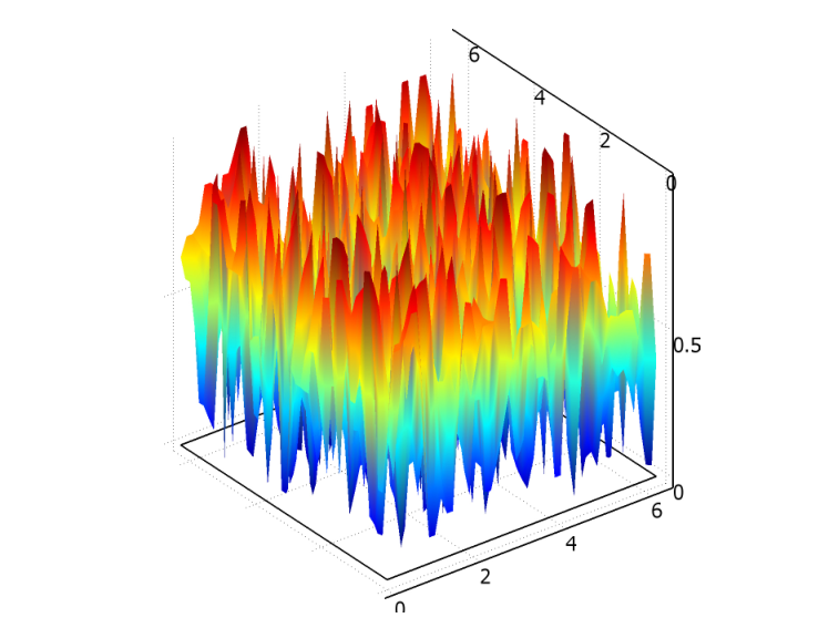
An extra term (1−ϵ​r​a​n​d​f)(1-\epsilon\ randf) has been incorporated in the right hand side terms of each equation in (4.35) to introduce ϵ\epsilon-perturbations, where r​a​n​d​frandf assumes values in [0,1][0,1] (see e.g. Fig. 4) and ϵ\epsilon is the perturbation control parameter. We fix h=0.2h=0.2 and τ=0.1\tau=0.1 and we use quadratic finite elements ℙ2\mathbb{P}_{2} for ψ\psi, cc and u and linear finite elements ℙ1\mathbb{P}_{1} for pp in order to study the stability of the method. We perform three different computational stability tests (in Fig.5, Fig.6, Fig.7 and Fig.8).
Refer to caption
Figure 4: Random function.
(a) Error curves in Example 1
(b) Error curves in Example 2
Figure 5: Errors Curves of norm E​Eϵ,e​xEE_{\epsilon,ex}.
(a) Error curves in Example 1
(b) Error curves in Example 2
Figure 6: Errors Curves of norm Eϵ,a​p​pE_{\epsilon,app}.

In Fig. 5, the L2​(𝒬)L^{2}({\cal Q})-norm of the discrepancy between exact solution Φe​x=(Φe​x(s))s=1,4=(ue​x,pe​x,ψe​x,ce​x)\Phi_{ex}=(\Phi_{ex}^{(s)})_{s=1,4}=(\textbf{u}_{ex},p_{ex},\psi_{ex},c_{ex}) and its ϵ\epsilon-perturbation Φϵ=(Φϵ(s))s=1,4=(uϵ,pϵ,ψϵ,cϵ)\Phi_{\epsilon}=(\Phi_{\epsilon}^{(s)})_{s=1,4}=(\textbf{u}_{\epsilon},p_{\epsilon},\psi_{\epsilon},c_{\epsilon}) i.e. Eϵ,e​x​(Φϵ(s)−Φe​x(s))=‖Φϵ(s)−Φe​x(s)‖L2​(Q)E_{\epsilon,ex}\left(\Phi_{\epsilon}^{(s)}-\Phi_{ex}^{(s)}\right)=\left\|\Phi_{\epsilon}^{(s)}-\Phi_{ex}^{(s)}\right\|_{L_{2}(Q)}, for s=1,4s=1,4 are plotted versus ϵ\epsilon (which are shown for ϵ=0.01,0.05,0.1,0.15,0.2,0.3,0.4\epsilon=0.01,0.05,0.1,0.15,0.2,0.3,0.4). A linear dependence of errors on ϵ\epsilon is observed, indeed, Eϵ,e​x​(Φϵ(s)−Φe​x(s))≈ms​ϵE_{\epsilon,ex}\left(\Phi_{\epsilon}^{(s)}-\Phi_{ex}^{(s)}\right)\approx\ m_{s}\ \epsilon, for s=1,4s=1,4, where msm_{s} represents the slope of the error curve; refer to Table 7. In Fig. 6, the error Eϵ,a​p​p​(Φϵ(s)−Φa​p​p(s))=‖Φϵ(s)−Φa​p​p(s)‖L2​(Q)E_{\epsilon,app}\left(\Phi_{\epsilon}^{(s)}-\Phi_{app}^{(s)}\right)=\left\|\Phi_{\epsilon}^{(s)}-\Phi_{app}^{(s)}\right\|_{L_{2}(Q)}, for s=1,4s=1,4 between the approximate solution Φa​p​p=(Φa​p​p(s))s=1,4=(ua​p​p,pa​p​p,ψa​p​p,ca​p​p)\Phi_{app}=(\Phi_{app}^{(s)})_{s=1,4}=(\textbf{u}_{app},p_{app},\psi_{app},c_{app}) without random (i.e., OPENϵ=0)\epsilon=0) and Φϵ\Phi_{\epsilon}, are plotted against ϵ\epsilon. The same observation holds as in Fig. 5; refer also to Table 7.

Finally, in Fig. 7 and Fig. 8, the solutions are shown on a part of domain and at time t=1t=1 in order demonstrate stability with respect to perturbations. In Fig. 7, we fix y=π/2y=\pi/2 and xx varies for velocity and concentration, and t=1t=1, x=πx=\pi and yy varies for pressure and phase field. In Fig. 8 we fix x=1/2x=1/2 and yy varies for velocity and phase field, and x=1/2x=1/2 and yy varies. The graphs shows that the solution is stable.

Slope Eϵ,e​xE_{\epsilon,ex} Eϵ,a​p​pE_{\epsilon,app}
mum_{\textbf{u}} 0.17010.1701 0.17540.1754
mψm_{\psi} 0.86380.8638 0.88180.8818
Example 1 mcm_{c} 0.43410.4341 0.43710.4371
mpm_{p} 1.47381.4738 1.49131.4913
mum_{\textbf{u}} 0.06280.0628 0.06350.0635
mψm_{\psi} 0.12830.1283 0.13470.1347
Example 2 mcm_{c} 0.10180.1018 0.10650.1065
mpm_{p} 1.48771.4877 1.42361.4236
Table 7: Slopes of Norm L2L_{2} in Examples 11 and 22.
Figure 7: Solution curves for the different values of ϵ\epsilon in Example 22.
Figure 8: Solution curves for the different values of ϵ\epsilon in Example 11.

6 Concluding remarks

This paper presents a numerical investigation and resolution of the isothermal anisotropic solidification model (2.1). The purpose of this study is to validate the derived numerical scheme by performing its error and stability analysis. The model has been discretized with respect to spatial and time variables . The discretization result into a system of nonlinear ordinary differential equations. The resulting non-linear systems are solved by using a solver DASSL.

Second, the convergence and stability of the numerical scheme has been validated (both with respect to space and time variables) by considering two examples with known exact solutions. It is numerically demonstrated that the error estimates with respect to spatial coordinates are of order i+1i+1 for 𝐮{\bf u}, ψ\psi and cc and of order ii for pp, and the error estimates for time are of order 1 for (𝐮,p,ψ,c)({\bf u},p,\psi,c). Both of these numerical estimates are in excellent accordance with the estimates (4.36). The stability of the scheme has also been verified by introducing a random function, which varies between 0 and 1, in the model. It is found that the numerical scheme is completely stable and it has linear dependence with the increase in percentage error.

7 Declarations

Competing interests: The author declare that he has no competing interests.
Acknowledgments: The author is thankful to the journal for consideration of this manuscript.

References

  • [1] Zhu M. F., Ting D., Lee S. Y. and Hong C. P., “Modeling of solutal dendritic growth with melt convection”, Computers and Mathematics with Applications, Vol. 55, pp. 1620-1628, 2008.
  • [2] Sun D. K., Zhu M.F., Pan S.Y., Yang C.R. and Raabe D., “Lattice Boltzmann modeling of dendritic growth in forced and natural convection”, Computers and Mathematics with Applications, Vol. 61, pp. 3585-3592, 2011.
  • [3] Anderson D. M., McFadden G. B., Wheeler A. A., “A phase-field model of solidification with convection”, Physica D, Vol. 135, pp. 175-194, 2000.
  • [4] Belmiloudi A., “Method of characteristics and error estimates of the perturbation of given mean flow. Application of mathematics in Engineering and Business Sozopol”, Proceedings of the XXII Summer School, pp. 25-38, 1996.
  • [5] Belmiloudi A., “ Robin-type boundary control problems for the nonlinear Boussinesq type equations”, Journal of Mathematical Analysis & Applications, Vol. 273, pp. 428-456, 2002.
  • [6] Belmiloudi A., “ Robust and optimal control problems to a phase-field model for the solidification of a binary alloy with a constant temperature”, Journal of Dynamical & Control Systems, Vol. 10, pp. 453-499, 2004.
  • [7] Belmiloudi A., “Stabilization, optimal and robust control: Theory and Applications in Biological and Physical Systems”, Springer-Verlag, London, Berlin, 2008.
  • [8] Chen Z., Hoffmann K. H., “ An error estimate for a finite-element scheme for a phase field model”, IMA J. Numer. Anal., Vol. 14, pp. 243–255, 1994.
  • [9] Galindo V., Gerbeth G., Ammon W. V., Tomzig E., Virbulis J., “Crystal growth melt flow previous term control next term by means of magnetic fields”, Energy Conv. Manage. Vol. 43, pp. 309-316, 2002.
  • [10] Grujicic M., Cao G., Millar R. S., “Computer modelling of the evolution of dendrite microstructure in binary alloys during non-isotheraml solidification”, J. Materials synthesis and processing, Vol. 10, No. 4, 191-203, 2002.
  • [11] Gunzberger M., Ozugurlu E., Turner J., Zhang H., “Controlling transport phenomena in the Czochralski crystal growth process”, J. Crystal Growth, Vol. 234, pp. 47-62, 2002.
  • [12] Hadid H. B., Henry D., Kaddeche S., “Numerical study of convection in the horizontal Bridgman configuration under the action of a constant magnetic field. Part 1. Two dimensional flow”, J. Fluid Mech., Vol. 333, pp. 23-56, 1997.
  • [13] Petzold L. R., “A discription of DASSL: A differential/algebraic system solver”, Scientific computing, IMACS Trans. Sci. Comput., pp. 65-68, 1983.
  • [14] Li M., Takuya T., Omura N., Miwa K., ”Effects of magnetic field and electric current on the solidification of AZ91D magnesium alloys using an electromagnetic vibration technique”, J. of Alloys and Compounds, Vol. 487, pp. 187-193, 2009.
  • [15] Ramizer J. C., Beckermann C., Kerma A., Diepers H. J., “Phase-field modeling of binary alloy solidification with couple heat and solute diffusion”, Physical Review E, Vol 69, pp. (051607-1)-(051607-16), 2004.
  • [16] Ramizer J. C., Beckermann C., “Examination of binary alloy free dendritic growth theories with a phase-field model”, Acta Materialia, Vol. 53, pp. 1721-1736, 2005.
  • [17] Rappaz M., Rettenmayr M., “Simulation of solidification”, Current Opinion in Solid State and Materials Science, Vol. 3, pp. 275-282, 1998.
  • [18] Rasheed A., Belmiloudi A., Mahe F., ”Dynamics of dendrite growth in a binary alloy with magnetic field affect”, Discrete and Continuous Dynamical Systems, Vol. 2011, pp. 1224-1233, Special Issue, 2011.
  • [19] Rasheed A., Belmiloudi A., ”An analysis of the Phase-field model for isothermal binary alloy solidification with convection under the influence of magnetic field”, Journal of Mathematical Analysis & Applications, Vol. 390, pp. 244-273, 2012.
  • [20] Rasheed A., Belmiloudi A., ”Mathematical Modelling and Numerical Simulation of Dendrite Growth Using Phase-Field Method with a Magnetic Field Effect”, Communications in Computational Physics, Vol. 14, pp. 477-508, 2013.
  • [21] Rasheed A., Wahab, A., ”Numerical analysis of an isotropic phase-field model with magnetic-field effect”, C.R. Acad. Sci. Paris, Ser. I, Vol. 353, pp. 219-224, 2015.
  • [22] Rasheed A., Belmiloudi A., ”Phase-field method for computationally efficient modeling of the solidification of binary alloy with magnetic field effect”, In. Proceedings of the NumAn2010 Conference in Numerical Analysis; Recent Approaches to Numerical Analysis: Theory, Methods and Applications, (eds., V. Dougalis, E. Gallopoulos, A. Hadjidimos et al.), pp. 222-230, 2010.
  • [23] Roplekar J. K., Dantzig J. A., “A study of solidification with a rotating magnetic field”, Int. J. Cast Met. Res. Vol. 14, pp. 79-95, 2001.
  • [24] Prescott P. J., Incropera F. P., “Magnetically damped convection during solidification of a binary metal alloy”, Trans. ASME, Vol. 115, pp. 302-310, 1993.
  • [25] Sampath R., “The adjoint method for the design of directional binary alloy solidification processes in the presence of a strong magnetic field”, Thesis, Cornell University USA, 2001.
  • [26] Süli E., “Convergence and non-linear stability of Lagrange-Galerkin method for the Navier-Stokes equations.”, Numer. Math, Vol. 53, pp. 459-483, 1988.
  • [27] Takaki T., Fukuoka T., Tomita Y., “Phase-field Simulations during Directional Solidification of a Binary Alloy using Adaptive Finite Element Method”, J. Crystal Growth, Vol. 283, pp. 263-278, 2005.
  • [28] Temam,R., “Navier–Stokes Equations”, North-Holland, Amsterdam, 1977.
  • [29] Tonhardt R., Amberg G., “Simulation of natural convection effects on succinonitrile crystals”, Physical Review E, Vol. 62, No. 1, pp. 828-836, 2000.
  • [30] Tong X., Beckermann C., Kerma A., Li Q., “Phase-field simulations of dendritic crystal growth in a forced flow”, Physical Review E, Vol 63, pp. (061601-1)-(061601-16), 2001.
  • [31] Warren J. A., Boettinger W. J., “Prediction of dendritic growth and microsegregation patterns in a binary alloy using the phase-field method”, Acta metall. mater, Vol. 43, No. 2, pp. 689-703, 1995.
  • [32] Watanabe M., Vizman D., Friedrich J., Mueller G., “Large modification of crystal-melt interface shape during Si crystal growth by using electromagnetic Czochralski method”, J. Crystal Growth, Vol. 292, pp. 252-256, 2006.