Lackadaisical quantum walk for spatial search

It was suggested by Richard Feynman and Paul Benioff in $1982$ that computations based on the principles of quantum mechanics would be more efficient than a classical computer. Although in principle, a classical computer can simulate a reasonable size quantum system, it is not efficient. One of the keys to the success of building quantum computers is to have efficient quantum algorithms nielsen; giri to run on these devices. A significant achievement in this direction is realized when Peter Shor in $1994$ shor1; shor2 showed that a quantum algorithm can factorize a large number in polynomial-time. Then in $1996$ Grover grover1; grover2; radha1; korepin1; zhang came up with an algorithm which can search for a target element in an unsorted database of size $N$ in $\mathcal{O}(\sqrt{N})$ time, which is quadratically faster than the exhaustive classical search of running time $\mathcal{O}(N)$. In Grover search, an initial state is prepared on which Grover iterator(unitary operator) is acted repeatedly until the target state is achieved with significant success probability. This can be seen as a rotation of a state in a two-dimensional plane defined by the initial state and the target state.

Another search problem is when the elements of a database are distributed on a graph vertices childs; amba1; amba2; meyer; amba4. Grover search can be implemented with the help of quantum walks on a complete graph, where each vertex is connected to all other vertices by an edge and each vertex has a directed self-loop. Grover search can then be seen as a search on both the spaces of vertices and edges. However, Grover search is not suitable for spatial search. One such example is a two-dimensional lattice of $\sqrt{N}\times\sqrt{N}$ vertices. The naive argument shows that Grover algorithm will take $\mathcal{O}(\sqrt{N})$ iteration time to search for a target state. However each Grover query needs $\mathcal{O}(\sqrt{N})$ time to perform reflection operation. Therefore the total running time becomes $\mathcal{O}(N)$ beni, which is the same as the time taken by classical exhaustive search. However it has been shown am; amba1 that a recursive algorithm combined with amplitude amplification brassard can search a two-dimensional lattice in $\mathcal{O}\left(\sqrt{N}\log^{2}N\right)$ time, which is better than the exhaustive classical search but less efficient than the Grover algorithm by a factor of $\log^{2}N$. For dimensions $d\geq 3$ it can search one target in $\mathcal{O}(\sqrt{N})$ time steps with optimal speed.

Searching a graph by quantum walks(QW) portugal, which is the quantum version of classical random walks, has been an important technique in achieving the desired speed. Since the probability distribution of quantum walks spreads quadratically faster than the classical random walks it is expected that the search algorithms based on quantum walks would outperform classical search algorithms. There are two types of quantum walks, namely, discrete and continuous time quantum walks, both of them can search a two-dimensional lattice for a single target in $\mathcal{O}\left(\sqrt{N}\log N\right)$ time and $d\geq 3$-dimensional lattice in $\mathcal{O}\left(\sqrt{N}\right)$ time amba2; childs1. In the critical case of $d=2$ dimensions a factor of $\mathcal{O}\left(\sqrt{\log N}\right)$ improvement in time complexity has been achieved tulsi; amba3; wong1.

Recently lackadaisical quantum walk search has been introduced wong1; wong2; wong3, which reduced the running time of search on a two-dimensional lattice by a factor of $\mathcal{O}\left(\sqrt{\log N}\right)$. Motivated by this result we in this article numerically investigate lackadaisical quantum walk search in one and two-dimensional lattice space. In particular, we will investigate how much improvement in success probability and running time is possible for a search of a single target state in the one-dimensional lattice. And for two-dimensional lattice, we study the running time and success probability for the search of multiple target states. In the case of Grover algorithm when the number of target states $M$ are increased the running time decreases as $\mathcal{O}(\sqrt{\frac{N}{M}})$. Discrete-time quantum walk search for one of the multiple targets can be reduced to single target search case, but the running time increases by a factor of $\mathcal{O}\left(\log N\right)$ amba2. For recent works on the search of multiple targets arranged in a cluster by quantum/lackadaisical quantum walks see refs. rivosh; saha; nahi.

This article is arranged in the following fashion. In section II we briefly discuss quantum walk search. In section III we study lackadaisical quantum walk search on one-dimension with periodic boundary conditions. In section IV we discuss lackadaisical quantum walk search for multiple target states on a two-dimensional lattice and finally in section V we conclude.

Here we briefly discuss how discrete-time quantum walk can be exploited to search on a graph. We consider a Cartesian graph $G(V,E)$, however the discussion can be generalized to other graphs as well. The space of vertices $\mathcal{H}_{V}$ with dimensions $N$ is the the space of database where we want to define our quantum search. On $d$-dimensional Cartesian graph with periodic boundary conditions each vertex is attached to $2d$-edges. A walker on a vertex can move to $2d$ possible direction by one step at a time. Similar to the coin tossing in classical random walk here we have a $2d$-dimensional coin space $\mathcal{H}_{C}$. So the quantum walk is defined on the tensor product space $\mathcal{H}=\mathcal{H}_{C}\times\mathcal{H}_{V}$. For the search algorithm we usually start with an initial state which is an equal superposition of the basis states on both the coin and vertex space

where $|\psi_{c}\rangle$ and $|\psi_{v}\rangle$ are the basis states of the coin space and vertex space respectively. We need to apply a suitably chosen unitary operator $\mathcal{U}$ on $|\psi_{in}\rangle$ till it reaches sufficiently close to the target state we are searching for. For the quantum walk

where $C$ is the coin operator which acts on the coin space as an unitary operator. Hadamard coin and Grover coin are some coin operators used in quantum walks. However, for the quantum search we have to distinguish the target states $|t_{v}\rangle$ from the non-target states, which we can do by applying two different coins, one to the target states and other to the non-target states. Another useful way is to apply the same coin $C_{1}$ on both types of states but with opposite signs

The shift operator $S$ moves the walker from one vertex to its immediate nearest neighbor vertices connected by $2d$-edges. However this shift operator is not efficient for search. Another one is the flip-flop shift operator, which besides shifting the walker from one vertex to the other it also inverts the direction as

As mentioned before in quantum search the final state is obtained after repeated application of $\mathcal{U}$ to the initial state

If $|\langle t_{v}|\psi_{f1}\rangle|\approx 1$, we reached to the target state with hight fidelity with the time complexity of the algorithm being $T_{1}$. In cases, where $|\langle t_{v}|\psi_{f1}\rangle|=1/T_{2}<<1$, amplitude amplification technique of Grover is used $T_{2}$ times to amplify the amplitude of the target state to $\mathcal{O}(1)$ in the evolving state. So, the total time complexity becomes $T=T_{1}T_{2}$. For the two-dimensional lattice $T_{1}=\mathcal{O}(\sqrt{N\log N})$ and $T_{2}=\mathcal{O}\left(\sqrt{\log N}\right)$, total time complexity is $T=\mathcal{O}(\sqrt{N}\log N)$ with $\mathcal{O}(1)$ success probability of the target state.

A one-dimensional lattice of size $N$ with periodic boundary conditions is the simplest model for search by quantum walk. The standard deviation for the quantum walk $\sigma{(t)}=t$ is quadratic compared to the standard deviation $\sigma{(t)}=\sqrt{t}$ of the corresponding classical random walk with after $t$ time steps. This ballistic spread of probabilities is a possible indication that the quantum walk would be faster than the classical walk. In the worst case scenario exhaustive classical search algorithm can find a target state in $\mathcal{O}(N)$ time. A classical algorithm based on the random walk can find a target state in $\mathcal{O}(N^{2})$ time. However a quantum algorithm based on quantum walk finds a target state in $\mathcal{O}(N)$ time but with $1/N$ success probability, which is not at all any improvement from the success probability of the target state in the initial state. Numerical simulation in ref. lovett for $N=50$ vertices on a line with periodic boundary conditions shows that the peak of success probability of about $2\pi/N$ is obtained for a search of single target state after about $5N$ time. They used a symmetric version of the Hadamard coin $H_{\gamma}^{1}$ with $\gamma=0.45$ for the transformation of the target state and $\gamma=0.5$ for the transformation of the non-target states.

Since the lackadaisical quantum walk improves the efficiency of searching on two-dimensional lattice wong3, we discuss how it works for a search on a one-dimensional lattice. We add one self-loop on each vertex of the lattice with a specific weight. The Hilbert space of the quantum coin $\mathcal{H}_{C}$ is spaned by the basis states $|x_{c}^{-}\rangle,|x_{c}^{+}\rangle,|x_{c}^{0}\rangle$ and the Hilbert space of the vertices $\mathcal{H}_{V}$ is given the basis states $|x_{v}\rangle$; $x_{v}\in[0,N-1]$. The quantum walker can go one step to the left, one step to the right or can stay in the same position as

where $S$ is the flip-flop shift operator, which can also be obtained from eq. (4) by putting $d=1$. Quantum search starts with an initial state

where the coin state $|\psi_{c}^{1D}\rangle$ is a weighted superposition of the coin basis

For the lackadaisical quantum walk we first need to rotate the coin state $|\psi_{c}^{1D}\rangle$ by a coin operator then the vertex state is evolved by the flip-flop shift operator $S$. We choose the Grover diffusion operator

for rotation of the coin state. To perform a search by LQW we have to devise a way to recognize the target state from the rest of the states, which we do by modifying the coin operator. We use $C_{G}$ for all basis states of vertex space except for the target state $|t_{v}\rangle$ in which case we use $-C_{G}$. We can express this modified coin operator as a single quantum coin operator as

Note that the operator $\tilde{C_{G}}$ acts not only on the coin space but also on the vertex space. The initial state evolves under the repeated application of the evolution operator

However the state thus obtained

has very low success probability in general for quantum walk searches with no self-loop. Slightly better success probability can be achieved by suitably choosing the coin operators as has been shown in ref. lovett by using biased Hadamard coin or symmetric version of the Hadamard coin

For $\delta=0$ eq. (III) is a biased Hadamard coin $H_{\gamma}^{0}$ and for $\delta=1$(positive square-root) it is a symmetric Hadamard coin $H_{\gamma}^{1}$. In FIG. 1(a) we have shown the variation of the success probability of the target state on a line of size $N=200$ with respect to the running time $T$. First peak of the success probability of $\approx 0.026$ is reached at $T=561$ for a coin $C_{sym}$ which acts as a symmetric Hadamard coin $H_{0.5}^{1}$ on the non-target states and $H_{0.4}^{1}$ on the target state

Numerical study on search by lackadaisical quantum walk shows more promising results. The first peak of the success probability of $\approx 0.75$ is reached at $T=200$ for a self-loop of $a=2/N$ in FIG. 1(b). The first peak of the success probability of $\approx 75$ percent(FIG. 2(b)) is reached in time $N$(FIG. 2(a)) for long range of the sizes $N\in\left[100,5000\right]$ of the one-dimensional lattice. Note that success probability of $\approx 75$ percent is almost constant for large $N$ and is fairly large compared to the search by regular quantum walk without self-loop. So the algorithm can find the target state in $\mathcal{O}(N)$ time steps.

Alternatively one can think of applying lackadaisical quantum walk till the success probability first reaches to $p_{s}=\mathcal{O}(1/\log N)$ and then apply amplitude amplification (brassard) $1/\sqrt{p_{s}}$ times to get success probability of $\mathcal{O}(1)$. In FIG. 3(b) blue square curve is the success probability when it first crosses the $\mathcal{O}(1/\log N)$ mark shown against the numbers of vertices $N$ on the lattice. The corresponding running time is plotted as blue square curve in FIG. 3(a). From the curve fitting it shows that the running time is $\mathcal{O}(N^{0.93010129})$ for a self-loop $a=2/N$. Since $\mathcal{O}(1/\log N)$ is a low success probability for large lattice size $N$ one has to apply amplitude amplification $\mathcal{O}\left(\sqrt{\log N}\right)$ times to achieve $\mathcal{O}(1)$ success probability, which increases the time complexity to $T=\mathcal{O}(N^{0.93010129}\sqrt{\log N})$. By a suitable curve fit again we obtain $T=\mathcal{O}(N^{0.98212135})\simeq\mathcal{O}(N)$, which is in good agreement with the result of the running time $\mathcal{O}(N)$ obtained in FIG. 2 using only lackadaisical quantum walk.

On a periodic $2$-dimensional lattice of size $\sqrt{N}\times\sqrt{N}$, there are $N$ vertex points $(x,y)$ and each vertex has $4$-edges. The collection of vertices is basically the unsorted database in our case and form the Hilbert space of vertices $\mathcal{H}_{V}$ with the basis states $|x_{v}^{1},x_{v}^{2}\rangle$. We add one self-loop to each vertex so the coin space has $5$ dimensions. The initial state for the purpose of the lackadaisical quantum walk is given by

where the coin state is

For the lackadaisical quantum walk we first need to rotate this coin state by a coin operator, which is followed by flip-flop shift operator to evolve the vertex state. We choose the Grover diffusion operator

for the rotation of the coin state. To recognize the target state from the rest of the states we modify the coin operator

where $|T_{M}\rangle=1/M\left(|t_{1}\rangle+|t_{2}\rangle+\cdots,|t_{M}\rangle\right)$ is the equal superposition of $M$ target states. The initial state after repeated application of $\mathcal{U}_{2D}$ becomes

where $\mathcal{U}_{2D}=S_{d=2}\tilde{C_{2D}}$. The shift operator $S_{d=2}$ can be readily obtained by putting $d=2$ in eq. (4).

In FIG. 4(a) numerical simulations for the running time for the cases $M=1$(green square curve), $M=2$(blue square curve) and $M=3$(cyan square curve) has been shown for the two-dimensional lattice size $\sqrt{N}=\left(10,11,\cdots,209\right)$ and their corresponding success probability to find one of the target states has been plotted in FIG. 4(b). Best fit for the running time shown by the red dashed curves in FIG. 4(a) for $M=1,2,3$ targets are given by

respectively for three target states $|\lfloor\sqrt{N}/2\rfloor,\lfloor\sqrt{N}/2\rfloor\rangle,|2,2\rangle$ and $|7,7\rangle$. We have also studied running time and sucess probability for $M=4,5$ and $6$ targets in FIG. 5 where $|\lfloor\sqrt{N}/2\rfloor,\lfloor\sqrt{N}/2\rfloor\rangle,|2,2\rangle$, $|7,7\rangle$, $|4,4\rangle$, $|8,8\rangle$ and $|10,10\rangle$ are the target states. Best fit for the running time shown in the red dashed curves in FIG. 5(a) are given by

The pre-factor for the running time in eqs. (24) and (25) increases slightly when the number of targets increase. Our numerical simulation results for multi target spacial search upto $M=6$ presented in eqs. (24) and (25) suggests that lackadaisical quantum walk can search one of the $M$ target states in

time steps. Note that we have chosen different values for the self-loop weight $a$ for different number of target states keeping large lattice size in mind, since we are interested in time complexity for large $N$. In the standard analysis of lackadaisical quantum walk search, the value of $a$ for which the first peak of the success probability is maximum, is chosen for the evaluation of the running time as has been presented in ref. wong3. This critical value of $a$ usually depends on the number of targets, the size of the lattice, the particular graph and its degree on which the quantum search is carried out. The variation of the success probability to find one of the target states as a function of $Na$ is shown in FIG. 6 for fixed $N$ and $M$.

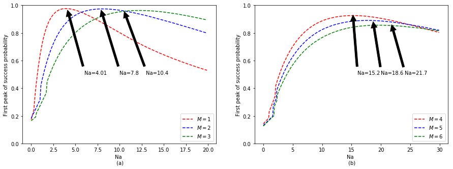
The success probabilities are close to the peaks for the values of $a$(self-loop) we have chosen in our analysis as can be seen from FIG. 6. Note that the success probabilities bellow about $N=2500$ slightly drop in FIG. 4 and 5, because our choices of the self-loop weight are not optimal for small lattice size.

Quantum walk has been an important tool for developing quantum search algorithms. On two-dimensional lattice, it has been observed that the regular quantum walk(no self-loop) searches a target state with $\mathcal{O}\left(\frac{1}{\log N}\right)$ success probability in $\mathcal{O}\left(\sqrt{N\log N}\right)$ time steps. Since this success probability is not significant we need to exploit amplitude amplification technique of Grover to get constant $\mathcal{O}(1)$ success probability at the cost of an increase of the running time by a factor of $\mathcal{O}\left(\sqrt{\log N}\right)$. The total time complexity is therefore $\mathcal{O}\left(\sqrt{N}\log N\right)$. One can improve the running time by introducing an ancilla qubit and modifying the quantum walk search tulsi so that constant $\mathcal{O}(1)$ success probability is achieved in $\mathcal{O}\left(\sqrt{N\log N}\right)$ time steps without involving amplitude amplification. Another approach is to consider a small neighborhood of the target state amba3, whose total probability is $\mathcal{O}(1)$ without further performing amplitude amplification.

Improvement of the running time has also been attributed to the laziness of the quantum walk in a recent work wong3 where a self-loop is attached on each vertex of the two-dimensional lattice. This approach, known as the lackadaisical quantum walk, has generated some interests in the critical case of $d=2$ dimensional lattice. We have studied the effect of laziness to search a target on a one-dimensional periodic lattice. It is known that quantum walk search in one-dimensional lattice is inefficient. However, our study shows that using the lackadaisical quantum walk we can increase the efficiency of the algorithm. In $N$ time steps it is possible to achieve a constant $\mathcal{O}(0.75)$ success probability exploiting only lackadaisical quantum walk with self-loop weight $a=2/N$(laziness), which is much better than to have a peak success probability of $2\pi/N$ after $2N$ or more time steps lovett by using regular quantum walk for search. Lackadaisical quantum walks followed by amplitude amplification can find a target state with $\mathcal{O}(1)$ success probability in $\mathcal{O}(N)$ time steps.

In two-dimensional lattice we have studied the effect of lackadaisical quantum walk to search one of the $M$ target states. The success probability and running time greatly varies as a function of the self-loop weight $a$ saha; nahi. However for some suitable choices of the self-loop weight one of the $M=1,2,3$ target states can be searched in $\mathcal{O}\left(\sqrt{\frac{N}{M}\log\frac{N}{M}}\right)$ time steps with $\mathcal{O}(1)$ success probability. We found that $T_{1}=0.76766755\sqrt{N\log N}$, $T_{2}=0.773523\sqrt{\frac{N}{2}\log\frac{N}{2}}$ and $T_{3}=0.87265627\sqrt{\frac{N}{3}\log\frac{N}{3}}$ are the best fit with the numerical data for the three target states $|\lfloor\sqrt{N}/2\rfloor,\lfloor\sqrt{N}/2\rfloor\rangle,|2,2\rangle$ and $|7,7\rangle$. We have also extended our analysis up to $M=6$ in FIG. 5. The choice of these target states is random in our numerical simulation, except for the cases of so-called exceptional configurations nahi of the target states for which there is no speedup. Note also that searching of $M$ targets arranged in a $\sqrt{M}\times\sqrt{M}$ group or uniformly distributed with a spacing of $\sqrt{N/M}$ between two targets have been studied rivosh, which shows that for the distributed case after $\mathcal{O}\left(\sqrt{\frac{N}{M}\log\frac{N}{M}}\right)$ time steps success probability of $\mathcal{O}\left(1/\log(N/M)\right)$ is achieved in regular quantum walk search. And for the grouped case $\Omega\left(\sqrt{N}-\sqrt{M}\right)$ time steps are required. The same system has also been studied saha by exploiting lackadaisical quantum walk, which gives better success probability. However, in our case, the arrangement of the targets does not have any specific restrictions on their arrangement.

It would be interesting to extend our study to other graph structures in two-dimensions to understand how the connectivity affects the success probability and running time in the presence of self-loop. Lattice without periodic boundary conditions is also another potential system to study search algorithm by lackadaisical quantum walk.

P. R. Giri is supported by International Institute of Physics, UFRN, Natal, Brazil. V. Korepin is grateful to SUNY Center of Quantum Information Science at Long Island for support.

References

- (1) M. A. Nielsen and I.L. Chuang, “Quantum Computation and Quantum Information”, (Cambridge: Cambridge University Press) (2000).
- (2) P. R. Giri and V. E. Korepin, Quantum Information Processing 16 1-36 (2017).
- (3) P. W. Shor, Polynomial-time algorithms for prime factorization and discrete logarithms on a quantum computer, Proc: 35th Annual Symposium on Foundations of Computer Science, Santa Fe, NM, 20-22, Nov. (1994).
- (4) P. W. Shor, SIAM J. Sci. Stat. Comput. 26 1484 (1997).
- (5) L. K. Grover, A fast quantum mechanical algorithm for database search, Pro. 28th Annual ACM Symp. Theor. Comput. (STOC) 212 (1996).
- (6) L. K. Grover, Phys. Rev. Lett. 79 325 (1997).
- (7) L. K. Grover and J. Radhakrishnan, ACM Symp. Parallel Algorithms and Architectures, Las Vegas, Nevada, USA 186 (2005).
- (8) B. S. Choi and V. E. Korepin, Quantum Inf. Process. 6 37 (2007).
- (9) K. Zhang, V. E. Korepin, Quantum Inf. Process. 17 143 (2018).
- (10) A. M. Childs and J. Goldstone, Phys. Rev. A 70 022314 (2004).
- (11) S. Aaronson and A. Ambainis, Proc. 44th IEEE Sympo-sium on Foundations of Computer Science, 200?209 (2003).
- (12) S. Aaronson and A. Ambainis, Theor. Comput. 1(4) 47-79 (2005).
- (13) A. Ambainis, J. Kempe and A. Rivosh, Proceedings 16th Annual ACM-SIAM Symposium Discrete Algorithms, SODA 05, 1099-1108. SIAM, Philadelphia, PA (2005).
- (14) D. A. Meyer and T. G. Wong, Phys. Rev. Lett. 114 110503 (2015).
- (15) S. Chakraborty, L. Novo, A. Ambainis and Yasser Omar, Phys. Rev. Lett. 116, 100501 (2016).
- (16) P. Benioff, Contemporary Mathematics 305 1?12, American Mathematical Society, Providence, RI (2002).
- (17) G. Brassard, P. Høyer, M. Mosca and A. Tapp, Quantum Amplitude Amplification and Estimation, Quantum computation and Quantum information, 305 53-74 (2000).
- (18) R. Portugal, Quantum Walks and Search Algorithms, Springer, New York (2013).
- (19) A. M. Childs and J. Goldstone, Phys. Rev. A 70, 042312 (2004).
- (20) A. Tulsi, Phys. Rev. A 78 012310 (2008).
- (21) A. Ambainis, A. Bakurs, N. Nahimovs, R. Ozols and A. Rivosh, Proceedings 7th Annual Conference Theory of Quantum Computation, Communication, and Cryptography, TQC 2012, 87–97. Springer, Tokyo (2013).
- (22) T. G. Wong, J. Phys. A Math. Theor. 48 43, 435304 (2015).
- (23) T. G. Wong, J. Phys. A Math. Theor. 50 47 475301 (2017).
- (24) T. G. Wong, Quantum Information Processing 17 68 (2018).
- (25) N. Nahimovs and A. Rivosh, Proceedings of SOFSEM, 9587 381-391 (2016).
- (26) A. Saha, R. Majumdar, D. Saha, A. Chakrabarti, and S. Sur-Kolay, arXiv:1804.01446 [quant-ph].
- (27) N. Nahimovs, arXiv:1808.00672 [quant-ph].
- (28) N. B. Lovett, M. Everitt, M. Trevers, D. Mosby, D. Stockton and V. Kendon, Nat. Comput. 11 23-35 (2012).