\addunit\pixel

pixel \addunit\pixelspixels \addunit\voxelvoxel \addunitdB \addunitB \addunit\hounsfieldHU

Deep Bayesian Inversion

Computational uncertainty quantification for large scale inverse problems

Jonas Adler
Department of Mathematics
KTH - Royal institute of Technology
jonasadl@kth.se
Research and Physics, Elekta Ozan Öktem
Department of Mathematics
KTH - Royal institute of Technology
ozan@kth.se

Abstract

Characterizing statistical properties of solutions of inverse problems is essential for decision making. Bayesian inversion offers a tractable framework for this purpose, but current approaches are computationally unfeasible for most realistic imaging applications in the clinic. We introduce two novel deep learning based methods for solving large-scale inverse problems using Bayesian inversion: a sampling based method using a Wasserstein GAN with a novel mini-discriminator and a direct approach that trains a neural network using a novel loss function. The performance of both methods is demonstrated on image reconstruction in ultra low dose 3D helical CT. We compute the posterior mean and standard deviation of the 3D images followed by a hypothesis test to assess whether a “dark spot” in the liver of a cancer stricken patient is present. Both methods are computationally efficient and our evaluation shows very promising performance that clearly supports the claim that Bayesian inversion is usable for 3D imaging in time critical applications.

1 Introduction

In several areas of science and industry there is a need to reliably recover a hidden multidimensional model parameter from noisy indirect observations. A typical example is when imaging/sensing technologies are used in medicine, engineering, astronomy, and geophysics.

These inverse problems are often ill-posed, meaning that small errors in data may lead to large errors in the model parameter and there are several possible model parameter values that are consistent with observations. Addressing ill-posedness is critical in applications where decision making is based on the recovered model parameter, like in image guided medical diagnostics. Furthermore, many highly relevant inverse problems are large-scale; they involve large amounts of data and high-dimensional model parameter spaces.

Bayesian inversion

Bayesian inversion is a framework for assigning probabilities to a model parameter given data (posterior) by combining a data model with a prior model (section 2). The former describes how measured data is generated from a model parameter whereas the latter accounts for information about the unknown model parameter that is known beforehand. Exploring the posterior not only allows for recovering the model parameter in a reliable manner by computing suitable estimators, it also opens up for a complete statistical analysis including quantification of the uncertainty.

A key part of Bayesian inversion is to express the posterior using Bayes’ theorem, which in turn requires access to the data likelihood, a prior, and a probability measure for data. The data likelihood is often given from insight into the physics of how data is generated (simulator). The choice of prior (section 2.1) is less obvious but important since it accounts for a priori information about the true model parameter. It is also very difficult to specify a probability distribution for data, which is required by many estimators. Finally, the computational burden associated with exploring the posterior (section 2.2) prevents usage of Bayesian inversion in most imaging applications.

To exemplify the above, consider clinical 3D computed tomography imaging where the model parameter represents the interior anatomy and data is x-ray radiographs taken from various directions. A natural prior in this context is that the object (model parameter) being imaged is a human being, but explicitly handcrafting such a prior is yet to be done. Instead, current priors prescribe roughness or sparsity, which suppresses unwanted oscillatory behavior at the expense of finer details. Next, the model parameter is typically $512^{3}$ -dimensional and data is of at least same order of magnitude. Hence, exploring the posterior in a timely manner is challenging, e.g., uncertainty quantification in Bayesian inversion remains intractable for such large-scale inverse problems.

2 Statistical Approach to Inverse Problems

Uncertainty refers in general to the accuracy by which one can determine a model parameter. In an inverse problems, this rests upon the ability to explore the statistical distribution of model parameters given measured data. More precisely, the posterior probability of the model parameter conditioned on observed data describes all possible solutions to the inverse problem along with their probabilities [21, 19] and it is essential for uncertainty quantification.

Bayesian inversion uses Bayes’ theorem [19, Theorem 14] to characterize the posterior:

p(x\mid y)=\frac{p(x)p(y\mid x)}{p(y)}.

Here, $p(y\mid x)$ is given by the data model that is usually derived from knowledge about how data is generated and $p(x)$ is given by the prior model that represents information known beforehand about the true (unknown) model parameter.

A tractable property of Bayesian inversion is that small changes in data lead to small changes in the posterior even when the inverse problem is ill-posed in the classical sense [19, Theorem 16], so Bayesian inversion is stable. Different reconstructions can be obtained by computing different estimators from the posterior and there is also a natural framework for uncertainty quantification, e.g., by computing Bayesian credible sets.

The posterior is however quite complicated with no closed form expression, so much of the contemporary research focuses on realizing the aforementioned advantages with Bayesian inversion without requiring access to the full posterior, see [19] for a nice survey. Some related key challenges were mentioned earlier in the introduction; choosing a “good” prior, specifying the probability distribution of data, and to explore the posterior in a computationally feasible manner.

2.1 Choosing a prior model

The difficulty in selecting a prior model lies in capturing the relevant a priori information. Bayesian non-parametric theory [25] provides a large class of handcrafted priors, but these only capture a fraction of the a priori information that is available. Figure 1 illustrates this by showing random samples generated from priors commonly used by state-of-the-art approaches in image recovery [37, 15] as well as samples from typical clinical computed tomography images. The handcrafted priors primarily encode regularity properties, like roughness or sparsity, and it would clearly be stretching our imagination to claim that corresponding samples represent natural images.

2.2 Computational feasibility

Exploring the posterior for inverse problems in imaging often leads to large scale numerics since this mounts to sampling from a high dimensional probability distribution. Most approaches, see section 6, are either not fast enough or rely on simplifying assumptions that does not hold in many applications For the above reasons, in large scale inverse problems one tends to reconstruct a single point estimate of the posterior distribution, the most common being the maximum a posteriori estimator that corresponds to the most likely reconstruction given the data. A drawback that comes with working with single estimators is that these cannot include all the information present in the posterior distribution. It is clear that knowledge about the full posterior would have dramatic impact upon how solutions to inverse problems are intertwined into decision making. As an example, in medical imaging, practitioners would be able to compute the probability of a tumor being an image artifact, which in turn is necessary for image guided hypothesis testing.

3 Contribution

Our overall contribution is to suggest two generic, yet adaptable, frameworks for uncertainty quantification in inverse problems that are computationally feasible and where both the prior and probability distribution of data are given implicitly through supervised examples instead of being handcrafted. The approach is based on recent advances in generative adversarial networks from deep learning and we demonstrate its performance on ultra low dose 3D helical computed tomography.

Our main contribution is Deep Posterior Sampling (section 4.1) where generative models from machine learning are used to sample from a high-dimensional unknown posterior distribution in the context of Bayesian inversion. This is made possible by a novel conditional Wasserstein GAN discriminator (section C.2). The approach is generic and applies in principle to any inverse problem assuming there is relevant training data. It can be used for performing statistical analysis of the posterior on $X$ , e.g., by computing various estimators.

Independently, we also introduce Deep Direct Estimation (section 4.2) where one directly computes an estimator using an deep neural network trained using a cleverly chosen loss (section C.3). Deep direct estimation is faster than posterior sampling, but it mainly applies to statistical analysis that is based on evaluating a pre-determined estimator. Both approaches should give similar quantitative results when used for evaluating the same estimator.

We demonstrate the performance and computational feasibility for ultra low dose computed tomography imaging in a clinical setting by computing some estimators and performing a hypothesis test (section 5).

4 Deep Bayesian Inversion

As already stated, in Bayesian inversion both the model parameter $x$ and measured data $y$ are assumed to be generated by random variables $\mathsf{x}$ and $\mathsf{y}$ , respectively. The ultimate goal is to recover the posterior $\pi(\mathsf{x}\mid y)$ , which describes all possible solutions $\mathsf{x}=x$ along with their probabilities given data $\mathsf{y}=y$ .

We here outline two approaches that can be used to perform various statistical analysis on the posterior. Deep Posterior Sampling is a technique for learning how to sample from the posterior whereas Deep Direct Estimation learns various estimators directly.

4.1 Deep Posterior Sampling

The idea is to explore the posterior by sampling from a generator that is defined by a Wasserstein GAN, which has been trained using a conditional Wasserstein GAN discriminator.

To describe how a Wasserstein GAN can be used for this purpose, let data $y\in Y$ be fixed and assume that $\pi(\mathsf{x}\mid y)$ , the posterior of $\mathsf{x}$ at $\mathsf{y}=y$ , can be approximated by elements in a parametrized family $\{\mathcal{G}_{\theta}(y)\}_{\theta\in\Theta}$ of probability measures on $X$ . The best such approximation is defined as $\mathcal{G}_{\theta^{*}}(y)$ where $\theta^{*}\in\Theta$ solves

\theta^{*}\in\argmin_{\theta\in\Theta}\,\ell\bigl(\mathcal{G}_{\theta}(y),\pi(\mathsf{x}\mid y)\bigr).

(1)

Here, $\ell$ quantifies the “distance” between two probability measures on $X$ . We are however interested in the best approximation for “all data”, so we extend eq. 1 by including an averaging over all possible data. The next step is to choose a distance notion $\ell$ that desirable from both a theoretical and a computational point of view. As an example, the distance should be finite and computational feasibility requires using it to be differentiable almost everywhere, since this opens up for using stochastic gradient descent type of schemes. The Wasserstein 1-distance $\Wasserstein$ (appendix A) has these properties [8] and sampling from the posterior $\pi(\mathsf{x}\mid y)$ can then be replaced by sampling from the probability distribution $\mathcal{G}_{\theta^{*}}(y)$ where $\theta^{*}$ solves

\theta^{*}\in\argmin_{\theta\in\Theta}\,\Expect_{\mathsf{y}\sim\sigma}\Bigl[\Wasserstein\bigl(\mathcal{G}_{\theta}(\mathsf{y}),\pi(\mathsf{x}\mid\mathsf{y})\bigr)\Bigr].

(2)

In the above, $\sigma$ is the probability distribution for data and $\mathsf{y}\sim\sigma$ generates data.

Observe now that evaluating the objective in eq. 2 requires access to the very posterior that we seek to approximate. Furthermore, the distribution $\sigma$ of data is often unknown, so an approach based on eq. 2 is essentially useless if the purpose is to sample from an unknown posterior. Finally, evaluating the Wasserstein 1-distance directly from its definition is not computationally feasible.

On the other hand, as shown in section C.1, all of these drawbacks can be circumvented by rewriting eq. 2 as an expectation over the joint law $(\mathsf{x},\mathsf{y})\sim\mu$ . This makes use of specific properties of the Wasserstein 1-distance (Kantorovich-Rubenstein duality) and one obtains the following approximate version of eq. 2:

\theta^{*}\in\argmin_{\theta\in\Theta}\Biggl\{\sup_{\phi\in\Phi}\Expect_{(\mathsf{x},\mathsf{y})\sim\mu}\biggl[\Discriminator_{\phi}(\mathsf{x},\mathsf{y})-\Expect_{\mathsf{z}\sim\eta}\bigl[\Discriminator_{\phi}(\Generator_{\theta}(\mathsf{z},\mathsf{y}),\mathsf{y})\bigr]\biggr]\Biggr\}.

(3)

In the above, $\Generator_{\theta}\colon Z\times Y\to X$ (generator) is a deterministic mapping such that $\Generator_{\theta}(\mathsf{z},y)\sim\mathcal{G}_{\theta}(y)$ , where $\mathsf{z}\sim\eta$ is a ‘simple’ $Z$ -valued random variable in the sense that it can be sampled in a computationally feasible manner. Next, the mapping $\Discriminator_{\phi}\colon X\times Y\to\mathbb{R}$ (discriminator) is a measurable mapping that is $1$ -Lipschitz in the $X$ -variable.

On a first sight, it might be unclear why eq. 3 is better than eq. 2 if the aim is to sample from the posterior, especially since the joint law $\mu$ in eq. 3 is unknown. The advantage becomes clear when one has access to supervised training data for the inverse problem, i.e., i.i.d. samples $(x_{1},y_{1}),\ldots,(x_{m},y_{m})$ generated by the random variable $(\mathsf{x},\mathsf{y})\sim\mu$ . The $\mu$ -expectation in eq. 3 can then be replaced by an averaging over training data.

To summarize, solving eq. 3 given supervised training data in $X\times Y$ amounts to learning a generator $\Generator_{\theta^{*}}(\mathsf{z},\cdot)\colon Y\to X$ such that $\Generator_{\theta^{*}}(\mathsf{z},y)$ with $\mathsf{z}\sim\eta$ is approximately distributed as the posterior $\pi(\mathsf{x}\mid y)$ . In particular, for given $y\in Y$ we can sample from $\pi(\mathsf{x}\mid y)$ by generating values of $z\mapsto\Generator_{\theta^{*}}(z,y)\in X$ in which $z\in Z$ is generated by sampling from $\mathsf{z}\sim\eta$ .

An important part of the implementation is the concrete parameterizations of the generator and discriminator:

\Generator_{\theta}\colon Z\times Y\to X\quad\text{and}\quad\Discriminator_{\phi}\colon X\times Y\to\mathbb{R}.

We here use deep neural networks for this purpose and following [27], we softly enforce the 1-Lipschitz condition on the discriminator by including a gradient penalty term to the training objective in eq. 3. Furthermore, if eq. 3 is implemented as is, then in practice $\mathsf{z}$ is not used by the generator (so called mode-collapse). To solve this problem, we introduce a novel conditional mini-batch discriminator that can be used with conditional WGAN without impairing upon its analytical properties (1), see section C.2 for more details.

4.2 Deep Direct Estimation

The idea here is to train a deep neural network to directly approximate an estimator of interest without resorting to generating samples from the posterior as in posterior sampling (section 4.1).

Deep direct estimation relies on the well known result:

\Expect_{\mathsf{w}}\bigl[\mathsf{w}\mid\mathsf{y}=\cdot\bigr]=\!\!\min_{\DeepVariation\colon Y\to W}\Expect_{(\mathsf{y},\mathsf{w})}\Bigl[\bigl\|\DeepVariation(\mathsf{y})-\mathsf{w}\bigr\|_{W}^{2}\Bigr].

(4)

In the above, $\mathsf{w}$ is any random variable taking values in some measurable Banach space $W$ and the minimization is over all $W$ -valued measurable maps on $Y$ . See proposition 2 in section C.3 for a precise statement. This is useful since many estimators relevant for uncertainty quantification are expressible using terms of this form for appropriate choices of $\mathsf{w}$ .

Specifically, section C.3 considers two (deep) neural networks $\ForwardOp^{\dagger}_{\theta^{*}}\colon Y\to X$ and $\DeepVariation_{\phi^{*}}\colon Y\to X$ with appropriate architectures that are trained according to

	$\displaystyle\theta^{*}\in$	$\displaystyle\ \argmin_{\theta}\biggl\{\Expect_{(\mathsf{x},\mathsf{y})\sim\mu}\Bigl[\bigl\\|\mathsf{x}-\ForwardOp^{\dagger}_{\theta}(\mathsf{y})\bigr\\|_{X}^{2}\Bigr]\biggr\}$
	$\displaystyle\phi^{*}\in$	$\displaystyle\ \argmin_{\phi}\biggl\{\Expect_{(\mathsf{x},\mathsf{y})\sim\mu}\Bigl[\bigl\\|\DeepVariation_{\phi}(\mathsf{y})-\bigl(\mathsf{x}-\ForwardOp^{\dagger}_{\theta^{*}}(\mathsf{y})\bigr)^{2}\bigr\\|_{X}^{2}\Bigr]\biggr\}.$

The resulting networks will then approximate the conditional mean and the conditional point-wise variance, respectively. Finally, if one has supervised training data $(x_{i},y_{i})$ , then the joint law $\mu$ above can be replaced by its empirical counterpart and the $\mu$ -expectation is replaced by an averaging over training data.

As already indicated, by using eq. 4 it is possible to re-write many estimators as minimizers of an expectation. Such estimators can then be approximated using the direct estimation approach outlined here. This should coincide with computing the same estimator by posterior sampling (section 4.1). Direct estimation is however significantly faster, but not as flexible as posterior sampling since each estimator requires a new neural network that specifically trained for that estimator. Section 5 compares outcome from both approaches.

5 Numerical Experiments

We evaluate the feasibility of posterior sampling (section 4.1) to sample from the posterior and Direct Estimation (section 4.2) to compute mean and point-wise variances for clinical 3D computed tomography imaging.

5.1 Set-up

Our supervised data consists of pairs of 3D computed tomography images $(x_{i},y_{i})$ generated by $(\mathsf{x},\mathsf{y})$ where $x_{i}$ is a normal dose 3D image that serves as the ‘ground truth’ and $y_{i}$ is the filtered back-projection 3D reconstruction computed from ultra low dose computed tomography data associated with $x_{i}$ .

One could here let $y_{i}$ be the ultra low dose computed tomography data itself, which results in more complex architectures of the neural networks. On the other hand, using filtered back-projection as a pre-processing step (i.e., $y_{i}$ is filtered back-projection reconstruction from ultra low dose data) simplifies the choice of architectures and poses no limitation in the theoretical setting with infinite data (see [4, section 8]).

Training data

We used training data from the Mayo Clinic Low Dose computed tomography challenge [47]. This data consists of ten computed tomography scans, of which we use nine for training and one for evaluation. Each 3D image $x_{i}$ has a corresponding ultra low dose data that is generated by using only $\approx 10\%$ of the full data and adding additional Poisson noise so that the dose corresponds to $2\%$ of normal dose. Applying filtered back-projection on this data yields the ultra low dose computed tomography images, see section D.1 for a detailed description.

An example of normal dose computed tomography reconstruction, tomographic data, and the ultra low dose filtered back-projection reconstruction is shown in fig. 2.

Network architecture and training

The operators

	$\displaystyle\Generator_{\theta}$	$\displaystyle\colon Z\times Y\to X$	$\displaystyle\qquad\qquad\ForwardOp^{\dagger}_{\theta^{*}}$	$\displaystyle\colon Y\to X$
	$\displaystyle\Discriminator_{\phi}$	$\displaystyle\colon X\times Y\to\mathbb{R}$	$\displaystyle\qquad\qquad\DeepVariation_{\phi^{*}}$	$\displaystyle\colon Y\to X$

are represented by multi-scale residual neural networks. For computational reasons, we applied the method slice-wise, see section D.2 for details regarding the exact choice of architecture and training procedure.

The parts related to the inverse problem (tomography) were implemented using the ODL framework [2] with ASTRA [62] as back-end for computing the ray-transform and its adjoint. The learning components were implemented in TensorFlow [1].

5.2 Results

Estimators

A typical use-case of Bayesian inversion is to compute estimators from the posterior. In our case, we are interested in the conditional mean and point-wise standard deviation (square root of variance).

When using posterior sampling, we compute the conditional mean and point-wise standard deviations based on 1 000 images sampled from the posterior, see appendix B for some examples of such images. For direct estimation we simply evaluated the associated trained networks. Both approaches are computationally feasible, the time needed per slice to compute these estimators is $40\text{\,}\mathrm{s}$ using posterior sampling based on 1 000 samples and $80\text{\,}\mathrm{ms}$ for direct estimation.

The mean and standard-deviations that were computed using both methods are shown in fig. 3. We note that results from the methods agree very well with each other, indicating that the posterior samples follow the posterior quite well, or at least that the methods have similar bias. The posterior mean looks as one would expect, with highly smoothed features due to the high noise level. Likewise, the standard deviation is also as one would expect, with high uncertainties around the boundaries of the high contrast objects. We also note that the standard deviation at the white “blobs” that appear in some samples (see appendix B) is quite high, indicating that the model is uncertain about their presence. There is also a background uncertainty at $\approx$20\text{\,}\hounsfield$$ due to point-wise noise in the reference normal-dose scans that we take as ground truth.

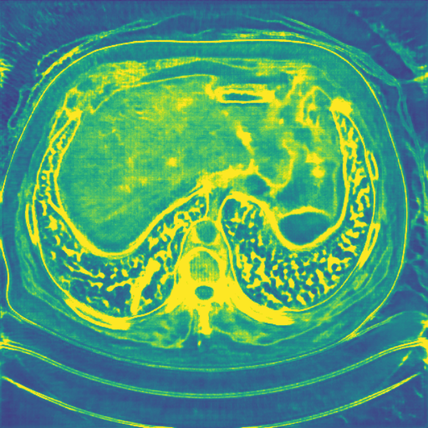Uncertainty quantification

We here show how to use Bayesian credible sets for clinical image guided decision making. One computes a reconstruction from ultra low dose data (middle image in fig. 2), identifies one or more features, and then seeks to estimate the likelihood for the presence of these features.

Formalizing the above, let $\Delta$ denote the difference in mean intensity in the reconstructed image between a region encircling the feature and the surrounding organ, which in our example is the liver. The feature is said to “exist” whenever $\Delta$ is bigger than a certain threshold, say $10\text{\,}\hounsfield$ .

To use posterior sampling, start by computing the conditional mean image (top left in fig. 3) by sampling from the posterior using the conditional Wasserstein GAN approach in section 4.1. There is a dark “spot” in the liver (possible tumor) and a natural clinical question is to statistically test for the presence of this feature. To do this, compute $\Delta$ for a number of samples generated by posterior sampling, which here is the same 1 000 samples used for computing the conditional mean. We estimate $p:=\Prob(\Delta>$10\text{\,}\hounsfield$)$ from the resulting histogram in fig. 4 and clearly $p>0.95$ , indicating that the “dark spot” feature exists with at least 95% significance. This is confirmed by the ground truth image (left image in fig. 2). The conditional mean image also under-estimates $\Delta$ , whose true value is the vertical line in fig. 4. This is to be expected since the prior introduces a bias towards homogeneous regions, a bias that decreases as noise level decreases.

To perform the above analysis using direct estimation, start with computing the conditional mean image from the same ultra-low dose data using direct estimation. As expected, the resulting image (top right in fig. 3) shows a dark “spot” in the liver. Now, designing and training a neural network that directly estimates the distribution of $\Delta$ is unfeasible in a general setting. However, as shown in section 4.2, this is possible if one assumes pixels are independent of each other. The estimated distribution of $\Delta$ is the curve in fig. 4 and we get $p>0.95$ , which is consistent with the result obtained using posterior sampling. The direct estimation approach is based on assuming independent pixels, so it will significantly underestimate the variance. In contrast, the approach based on posterior sampling seems to give a more realistic estimate of the variance.

6 Related Work

Deep learning based methods are increasingly used for medical image reconstruction, either by using deep learning for post-processing [38, 35] or by integrating deep learning into the image reconstruction [66, 5, 6, 29, 16, 28, 30]. These papers start by specifying the loss and then use a deep neural network to minimize the expected loss. This essentially amounts to directly computing a Bayes estimator with a risk is given by the loss. The loss is often the squared $L_{2}$ -distance, which implicitly implies that one approximates the conditional mean. Hence, the above approaches could be seen as examples of deep direct estimation. There is however an important difference, in deep direct estimation one starts by explicitly specify the estimator, which then implies the appropriate loss function.

There has also been intense research in selecting a loss function different from the $L_{2}$ -loss [36, 7] and specifically generative adversarial network-like methods have been applied to image post-processing in computed tomography [64, 67] and image reconstruction in magnetic resonance imaging (Fourier inversion) [65, 46]. However, in these papers the authors discard providing any randomness to the generator, instead only giving it the prior. They have thus not fully realized the potential of using generative adversarial networks for sampling from the posterior in Bayesian inversion.

Regarding sampling from a posterior, conditional generative models [48, 49] have been widely used in the machine learning literature for this purpose. Typical use cases is to sample from a posterior where an image is conditioned on a text, like “the bird is yellow” [32, 20], but also for simple applications in imaging, including image super-resolution and in-painting [44, 52, 51]. These approaches do not consider sampling from the posterior for more elaborate inverse problems that involve a physics driven data likelihood. An approach in this direction is presented in [41] where variational auto-encoders are used to sample from the posterior of possible segmentations (model parameter) given computed tomography images (data).

An entirely different class of methods for exploring the posterior are based on Markov chain Monte Carlo techniques, which have revolutionized mathematical computation and enabled statistical inference within many previously intractable models. Most of the techniques are rooted in solid mathematical theory, but they are limited to cases where the prior model is known in closed form, see surveys in [19, 15, 11]. Furthermore, these Markov chain Monte Carlo techniques are still computationally unfeasible for large-scale inverse problems, like 3D clinical computed tomography.

A computationally feasible alternative to Markov chain Monte Carlo for uncertainty quantification is to consider asymptotic characterizations of the posterior. For many inverse problems, it is possible to prove Bernstein–von Mises type of theorems that characterizes the posterior using analytic expressions assuming the prior is asymptotically uninformative [50]. Such characterizations do not hold for finite data, but assuming a Gaussian process model (data likelihood and prior are both Gaussian) allows for using numerical methods for linear inverse problems [55]. Gaussian process models are however still computationally demanding and it can be hard to design appropriate priors, so [23, 24] introduces (conditional) neural processes that incorporate deep neural networks into Gaussian process models for learning more general priors.

Finally, another computationally feasible approach for uncertainty quantification is to approximate Bayesian credible sets for the maximum a posteriori estimator by solving a convex optimization problem [57, 54]. The approach is however restricted to the maximum a posteriori estimator and furthermore, it requires access to a handcrafted prior.

7 Conclusions

Bayesian inversion is an elegant framework for recovering model parameters along with uncertainties that applies to a wide range of inverse problems. The traditional approach requires specifying a prior and, depending on the choice of estimator, also the probability of data. Furthermore, exploring the posterior remains a computational challenge. Hence, despite significant progress in theory and algorithms, Bayesian inversion remains unfeasible for most large scale inverse problems, like those arising in imaging.

This paper addresses all these issues, thereby opening up for the possibility to perform Bayesian inversion on large scale inverse problems. Capitalizing on recent advances in deep learning, we present two approaches for performing Bayesian inversion: Deep Posterior Sampling (section 4.1), which uses a generative adversarial network to sample from the posterior, and Deep Direct Estimation (section 4.2) that computes an estimator directly using a deep neural network.

The performance of both approaches is demonstrated in the context of ultra low dose ( $2\%$ of normal dose) clinical 3D helical computed tomography imaging (section 5). We show how to compute basic Bayesian estimators, like the posterior mean and point-wise standard deviation. We also compute Bayesian credible sets and use this for testing whether a suspected “dark spot” in the liver, which is visible in the posterior mean image, is real. The quality of the posterior mean reconstruction is also quite promising, especially bearing in mind that it is computed from computed tomography data that corresponds to $2\%$ of normal dose.

To the best of our knowledge, this is the first time one can perform such computations on large scale inverse problems in a timely manner, like clinical 3D helical computed tomography image reconstruction. On the other hand, using such a radically different way to perform image reconstruction in clinical practice quickly gets complicated since it must be preceded by clinical trials in the context of image guided decision making. However, there are many advantages that comes with using our proposed approach, which for medical imaging means integrating imaging with clinical decision making while accounting for the uncertainty.

To conclude, the posterior sampling approach allows one to perform Bayesian inversion on large scale inverse problems that goes beyond computing specific estimators, such as the maximum a posteriori or conditional mean. The framework is not specific to tomography, it applies to essentially any inverse problem assuming access to sufficient amount of “good” supervised training data. Furthermore, the possibility to efficiently sample from the posterior opens up for new ways to integrate decision making with reconstruction.

8 Discussion and Outlook

There are several open research topics related to using generative adversarial networks as generative models for the posterior in inverse problems.

One natural topic is to have a precise notion of “good” supervised training data. Specifically, it is desirable to estimate the amount of supervised training data necessary for “resolving” the posterior/estimator up to some accuracy. Unfortunately, most of the current theory for Bayesian inference does not apply directly to this setting. Its emphasis is on characterizing the posterior in the asymptotic regime where information content in data increases indefinitely and the prior is asymptotically non-informative, like when a Gaussian prior is used.

Another research topic is to study whether there are theoretical guarantees that ensure the conditional Wasserstein GAN generator given by eq. 3 converges towards the posterior. In [26] one proves that given infinite capacity of the discriminator, the optimal generator minimizes the Jensen–Shannon divergence w.r.t. the target distribution. For the case with Wasserstein GAN, [56, Lemma 6] shows that one can learn the posterior in the sense of [60, Definition 3.1], i.e. solving eq. 10 arbitrarily well, given enough training data. But this does not settle the question of what happens with realistic sample and model capacities. This is part of a more general research theme for investigating the theoretical basis for using generative adversarial networks trained on supervised data to sample from high dimensional probability distributions [9].

Yet another topic relates to including explicit knowledge about the data likelihood, which in contrast to the prior, can be successfully handcrafted for many inverse problems. This is essential for large-scale inverse problems where the amount of supervised training data is little and there are few opportunities for re-training when data the acquisition protocol changes. In this work, this knowledge was implicitly accounted for by our choice to use a filtered back-projection reconstruction as the data. While it can be proven that this is in theory sufficient for generating samples from the posterior [4, section 8], [5, 6] clearly shows that working directly from measured data gives better results. We therefore expect further improvements to our results by using a conditional Wasserstein GANs based on convolutional neural network architectures that integrate a handcrafted data likelihood, such as those provided by learned iterative reconstruction.

Finally, our deep direct estimators were very easy to train with no major complications, but training the generative models for posterior sampling is still complicated and involves quite a bit of fine tuning and “tricks”. We hope that future research in generative models will improve upon this situation.

Acknowledgments*

The work was supported by the Swedish Foundation of Strategic Research grant AM13-0049, Industrial PhD grant ID14-0055 and by Elekta. The authors also thank Dr. Cynthia McCollough, the Mayo Clinic, and the American Association of Physicists in Medicine, and acknowledge funding from grants EB017095 and EB017185 from the National Institute of Biomedical Imaging and Bioengineering, for providing the data.

Appendices

Appendix A The Wasserstein 1-distance

Let $X$ be a measurable separable Banach Space and $\mathcal{P}_{X}$ the space of probability measures on $X$ . The Wasserstein 1-distance $\Wasserstein\colon\mathcal{P}_{X}\times\mathcal{P}_{X}\to\mathbb{R}$ is a metric on $\mathcal{P}_{X}$ that can be defined as [63, Definition 6.1]

\Wasserstein(p,q):=\!\!\inf_{\mu\in\Pi(p,q)}\Expect_{(\mathsf{x},\mathsf{v})\sim\mu}\bigl[\|\mathsf{x}-\mathsf{v}\|_{X}\bigr]\quad\text{for $p,q\in\mathcal{P}_{X}$.}

(5)

In the above, $\Pi(p,q)\subset\mathcal{P}_{X\times X}$ denotes the family of joint probability measures on $X\times X$ that has $p$ and $q$ as marginals. Note also that we assume $\mathcal{P}_{X}$ only contains measures where the Wasserstein distance takes finite values (Wasserstein space), see [63, Definition 6.4] for the formal definition.

The Wasserstein 1-distance in eq. 5 can be rewritten using the Kantorovich-Rubinstein dual characterization [63, Remark 6.5 on p. 95], resulting in

\Wasserstein(p,q)=\!\!\sup_{\vbox{\Let@\restore@math@cr\default@tag\halign{\hfil$\m@th\scriptstyle#$&$\m@th\scriptstyle{}#$\cr&\Discriminator\colon X\to\mathbb{R}\,\,\,\\ &\Discriminator \in\Lip($X$)\crcr}}}\Bigl\{\Expect_{\mathsf{x}\sim q}\bigl[\Discriminator(\mathsf{x})\bigr]-\Expect_{\mathsf{v}\sim p}\bigl[\Discriminator(\mathsf{v})\bigr]\Bigr\}\quad\text{for $p,q\in\mathcal{P}_{X}$.}

(6)

Here, $\Lip(X)$ denotes real-valued 1-Lipschitz maps on $X$ , i.e.,

\Discriminator\in\Lip(X)\quad\Longleftrightarrow\quad|\Discriminator(x_{1})-\Discriminator(x_{2})|\leq\|x_{1}-x_{2}\|_{X}\quad\text{for all $x_{1},x_{2}\in X$.}

The above constraint can be hard to enforce in eq. 6 as is, so following [27, 3] we prefer the gradient characterization:

\Discriminator\in\Lip(X)\quad\Longleftrightarrow\quad\bigl\|\partial\!\Discriminator(x)\bigr\|_{X^{*}}\leq 1\quad\text{for all $x\in X$,}

where $\partial$ indicates the Fréchet derivative and $X^{*}$ is the dual space of $X$ . In our setting, $X$ is an $L_{2}$ space, which is a Hilbert space so $X^{*}=X$ and the Fréchet derivative becomes the (Hilbert space) gradient of $\Discriminator$ .

Appendix B Individual Posterior Samples

It is instructive to visually inspect individual random samples of the posterior obtained from the conditional Wasserstein GAN generator.

Generating one such sample is fast, taking approximately $40\text{\,}\mathrm{ms}$ on a desktop “gaming” PC. Furthermore, as seen in fig. 5, the generated samples look realistic, practically indistinguishable from the ground truth to the untrained observer. With that said, some anatomical features are clearly misplaced, e.g., there are white “blobs” (blood vessels) in the liver. These are present because the supervised training set contained images from patients that were given contrast (see bottom row in fig. 1), which has influenced the anatomical prior that is learned from the supervised data.

Appendix C Theory of Deep Bayesian Inversion

This section contains the theoretical foundations needed for Deep Bayesian Inversion and derivations of the expressions used in the main article.

C.1 Derivation of conditional Wasserstein GAN

This section provides the mathematical details for deriving eq. 3 from eq. 2. Such a reformulation is well-known, but the derivation given here seems to be novel.

The overall aim with Wasserstein GAN is to approximate the posterior $y\mapsto\pi(\mathsf{x}\mid y)$ that is inaccessible. The approach is to construct a mapping that associates a probability measure on $X$ to each data $y\in Y$ . A family of such mappings can be explicitly constructed and trained against supervised training data in order to approximate the posterior. To proceed we need to specify the statistical setting and our starting point is to introduce a “distance” between two probability measures on $X$ :

\ell\colon\mathcal{P}_{X}\times\mathcal{P}_{X}\to\mathbb{R}_{+}.

(7)

In the above, $\mathcal{P}_{X}$ denotes the class of all probability measures on $X$ , so $\pi(\mathsf{x}\mid y)\in\mathcal{P}_{X}$ whenever the posterior exists, which holds under fairly general assumptions where both $X$ and $Y$ can be infinite-dimensional separable Banach spaces [19, Theorem 14]. Next, let $\GenProbMapSpace$ denote a fixed family of generators, which are mappings

\mathcal{G}\colon Y\to\mathcal{P}_{X}

(8)

that associate each $y\in Y$ to a probability measure on $X$ . Note here that $y\mapsto\pi(\mathsf{x}\mid y)$ is not necessarily contained in $\GenProbMapSpace$ . A generator in $\GenProbMapSpace$ is an “optimal” approximation of the posterior $y\mapsto\pi(\mathsf{x}\mid y)$ if it minimizes the expected $\ell$ -distance, i.e., it solves

\inf_{\mathcal{G}\in\GenProbMapSpace}\,\Expect_{\mathsf{y}\sim\sigma}\Bigl[\ell\bigl(\mathcal{G}(\mathsf{y}),\pi(\mathsf{x}\mid\mathsf{y})\bigr)\Bigr].

(9)

Here, $\mathsf{y}\sim\sigma$ is the $Y$ -valued random variable generating data.

There are three issues that arise if a solution to eq. 9 is to be used as a proxy for the posterior:

(i) Evaluating the objective requires access to the very posterior, which we assumed was inaccessible, (ii) the distribution

\sigma

of data is almost always unknown, so the expectation cannot be computed, and finally (iii) the computational feasibility requires access to an explicit finite dimensional parametrization for constructing generators in

\GenProbMapSpace

that one searches over in eq. 9.

As we shall see next, choosing eq. 7 as the Wasserstein 1-distance allows us to addresses the first two issues. With this choice one can re-write the objective in eq. 9 as an expectation over the joint law $(\mathsf{x},\mathsf{y})\sim\mu$ , thereby avoiding expressions that explicitly depend on the unknown posterior $y\mapsto\pi(\mathsf{x}\mid y)$ and distribution of data $\sigma$ . This joint law is also unknown, but it can often be replaced by its empirical counterpart derived from a suitable supervised training data set.

More precisely, choosing the Wasserstein 1-distance $\Wasserstein\colon\mathcal{P}_{X}\times\mathcal{P}_{X}\to\mathbb{R}_{+}$ as $\ell$ in eq. 9 yields

\inf_{\mathcal{G}\in\GenProbMapSpace}\,\Expect_{\mathsf{y}\sim\sigma}\Bigl[\Wasserstein\bigl(\mathcal{G}(\mathsf{y}),\pi(\mathsf{x}\mid\mathsf{y})\bigr)\Bigr].

(10)

Note here that $y\mapsto\Wasserstein\bigl(\mathcal{G}(y),\pi(\mathsf{x}\mid y)\bigr)$ is assumed to be a measurable real-valued function on $Y$ . The Kantorovich-Rubinstein dual characterization in eq. 6 yields

\Wasserstein\bigl(\mathcal{G}(y),\pi(\mathsf{x}\mid y)\bigr)=\!\!\!\sup_{\Discriminator_{y}\in\Lip(X)}\biggl\{\Expect_{\vbox{\Let@\restore@math@cr\default@tag\halign{\hfil$\m@th\scriptstyle#$&$\m@th\scriptstyle{}#$\cr&\mathsf{x}\sim\pi(\mathsf{x}\mid y)\\ &\mathsf{$v$}\sim\mathcal{G}($y$)\crcr}}}\bigl[\Discriminator_{y}(\mathsf{x})-\Discriminator_{y}(\mathsf{v})\bigr]\biggr\}\quad\text{for $y\in Y$.}

(11)

Here, $\Lip(X)$ denotes the set of real-valued mappings on $X$ that are 1-Lipschitz. Hence, eq. 10 can be written as

\inf_{\mathcal{G}\in\GenProbMapSpace}\,\Expect_{\mathsf{y}\sim\sigma}\Biggl[\sup_{\Discriminator_{\mathsf{y}}\in\Lip(X)}\biggl\{\Expect_{\vbox{\Let@\restore@math@cr\default@tag\halign{\hfil$\m@th\scriptstyle#$&$\m@th\scriptstyle{}#$\cr&\mathsf{x}\sim\pi(\mathsf{x}\mid\mathsf{y})\\ &\mathsf{$v$}\sim\mathcal{G}(\mathsf{$y$})\crcr}}}\bigl[\Discriminator_{\mathsf{y}}(\mathsf{x})-\Discriminator_{\mathsf{y}}(\mathsf{v})\bigr]\biggr\}\Biggr].

(12)

Next, in this case the supremum commutes with the $\sigma$ -expectation, i.e.,

\Expect_{\mathsf{y}\sim\sigma}\Biggl[\sup_{\Discriminator_{\mathsf{y}}\in\Lip(X)}\biggl\{\Expect_{\vbox{\Let@\restore@math@cr\default@tag\halign{\hfil$\m@th\scriptstyle#$&$\m@th\scriptstyle{}#$\cr&\mathsf{x}\sim\pi(\mathsf{x}\mid\mathsf{y})\\ &\mathsf{v}\sim\mathcal{G}(\mathsf{y})\crcr}}}\bigl[\Discriminator_{\mathsf{y}}(\mathsf{x})-\Discriminator_{\mathsf{y}}(\mathsf{v})\bigr]\biggr\}\Biggr]\\ =\sup_{\Discriminator\in\DiscrSpace(X\times Y)}\biggl\{\Expect_{\vbox{\Let@\restore@math@cr\default@tag\halign{\hfil$\m@th\scriptstyle#$&$\m@th\scriptstyle{}#$\cr&(\mathsf{x},\mathsf{y})\sim\mu\\ &\mathsf{v}\sim\mathcal{G}(\mathsf{y})\crcr}}}\Bigl[\Discriminator(\mathsf{x},\mathsf{y})-\Discriminator(\mathsf{v},\mathsf{y})\Bigr]\biggr\},

(13)

where $\DiscrSpace(X\times Y)$ is the space of measurable real-valued mappings on $X\times Y$ that are 1-Lipschitz in the $X$ -variable for every $y\in Y$ . The proof of eq. 13 is given on p. C.1 and combining it with eq. 12 gives

\inf_{\mathcal{G}\in\GenProbMapSpace}\,\Biggl\{\sup_{\Discriminator\in\DiscrSpace(X\times Y)}\Expect_{\vbox{\Let@\restore@math@cr\default@tag\halign{\hfil$\m@th\scriptstyle#$&$\m@th\scriptstyle{}#$\cr&(\mathsf{x},\mathsf{y})\sim\mu\\ &\mathsf{$v$}\sim\mathcal{G}(\mathsf{$y$})\crcr}}}\Bigl[\Discriminator(\mathsf{x},\mathsf{y})-\Discriminator(\mathsf{v},\mathsf{y})\Bigr]\Biggr\}.

(14)

Note that there are no approximations involved in going from eq. 10 to eq. 14, the derivation is solely based on properties of the Wasserstein 1-distance. Furthermore, the advantage of eq. 14 over eq. 10 is that the latter neither involves the posterior nor $\sigma$ (the probability measure of data). It does involve the joint law $(\mathsf{x},\mathsf{y})\sim\mu$ , which is of course unknown. On the other hand, if we have access to supervised training data:

(x_{1},y_{1}),\ldots,(x_{m},y_{m})\in X\times Y\quad\text{are i.i.d. samples of $(\mathsf{x},\mathsf{y})\sim\mu$,}

(15)

then we can replace the joint law $\mu$ in eq. 14 with its empirical counterpart and the $\mu$ -expectation is replaced by an averaging over training data.

The final steps concern computational feasibility. We start by considering parameterizations of the generators in $\GenProbMapSpace$ that enables one to solve eq. 14 in a computational feasible manner. A key aspect is to evaluate the $\mathcal{G}(y)$ -expectation for any $y\in Y$ without impairing upon the ability to approximate the posterior with elements from $\GenProbMapSpace$ . We will assume that each generator $\mathcal{G}\in\GenProbMapSpace$ corresponds to a measurable map $\Generator\colon Z\times Y\to X$ such that the following holds:

\mathsf{v}\sim\mathcal{G}(y)\iff\mathsf{v}=\Generator(\mathsf{z},y)\quad\text{for some $Z$-valued random variable $\mathsf{z}\sim\eta$.}

(16)

In the above, $Z$ is some fixed set and $\eta$ is a “simple” probability measure on $Z$ meaning that there are computationally efficient means for generating samples of $\mathsf{z}\sim\eta$ . It is then possible to express eq. 14 as

\inf_{\Generator\in\GeneratorSpace}\,\biggl\{\sup_{\Discriminator\in\DiscrSpace(X\times Y)}\Expect_{\vbox{\Let@\restore@math@cr\default@tag\halign{\hfil$\m@th\scriptstyle#$&$\m@th\scriptstyle{}#$\cr&(\mathsf{x},\mathsf{y})\sim\mu\\ &\mathsf{z}\sim\eta\crcr}}}\Bigl[\Discriminator(\mathsf{x},\mathsf{y})-\Discriminator\bigl(\Generator(\mathsf{z},\mathsf{y}),\mathsf{y}\bigr)\Bigr]\biggr\}

(17)

where $\GeneratorSpace$ is the class of $X$ -valued measurable maps on $Z\times Y$ that corresponds to $\GenProbMapSpace$ by eq. 16.

The formulation in eq. 17 involves taking the infimum over $\GeneratorSpace$ and supremum over $\DiscrSpace$ , which is clearly computationally unfeasible. Hence, one option is to consider a parametrization of these spaces using deep neural networks with appropriately chosen architectures:

	$\displaystyle\GeneratorSpace:=\{\Generator_{\theta}\}_{\theta\in\Theta}$	where	$\displaystyle\Generator_{\theta}\colon Z\times Y\to X\phantom{.}$		(18)
	$\displaystyle\DiscrSpace:=\{\Discriminator_{\phi}\}_{\phi\in\Phi}$	where	$\displaystyle\Discriminator_{\phi}\colon X\times Y\to\mathbb{R}.$		(19)

Inserting the above parametrizations into eq. 17 results in

\theta^{*}\in\argmin_{\theta\in\Theta}\,\biggl\{\sup_{\phi\in\Phi}\,\,\Expect_{\vbox{\Let@\restore@math@cr\default@tag\halign{\hfil$\m@th\scriptstyle#$&$\m@th\scriptstyle{}#$\cr&(\mathsf{x},\mathsf{y})\sim\mu\\ &\mathsf{z}\sim\eta\crcr}}}\Bigl[\Discriminator_{\phi}(\mathsf{x},\mathsf{y})-\Discriminator_{\phi}\bigl(\Generator_{\theta}(\mathsf{z},\mathsf{y}),\mathsf{y}\bigr)\Bigr]\biggr\}.

(20)

Note again that the unknown joint law $\mu$ in eq. 20 is replaced by its empirical counterpart given from the training data in eq. 15.

To summarize, solving the training problem in eq. 20 given training data eq. 15 and the parametrizations in eqs. 18 and 19 yields a mapping $\Generator_{\theta^{*}}\colon Z\times Y\to X$ that approximates the posterior in the sense that the distribution of $\Generator_{\theta^{*}}(\mathsf{z},y)$ with $\mathsf{z}\sim\eta$ is closest to $\pi(\mathsf{x}\mid y)$ in expected Wasserstein 1-distance. Hence, we can sample $z\in Z$ from $\mathsf{z}\sim\eta$ and $\Generator_{\theta^{*}}(z,y)\in X$ will approximate a sample of the conditional random variable $(\mathsf{x}\mid\mathsf{y}=y)\sim\pi(\mathsf{x}\mid y)$ . The formulation in eq. 20 is also suitable for stochastic gradient descent, so computational techniques from deep neural networks can be used for solving the empirical expected minimization problem. We conclude with providing a proof of eq. 13.

Proof of eq. 13

To simplify the notational burden, define $f_{\Discriminator}\colon Y\to\mathbb{R}$ as

f_{\Discriminator}(y):=\Expect_{\vbox{\Let@\restore@math@cr\default@tag\halign{\hfil$\m@th\scriptstyle#$&$\m@th\scriptstyle{}#$\cr&\mathsf{x}\sim\pi(\mathsf{x}\mid y)\\ &\mathsf{$v$}\sim\mathcal{G}($y$)\crcr}}}\bigl[\Discriminator(\mathsf{x})-\Discriminator(\mathsf{v})\bigr]\quad\text{for $\Discriminator\in\Lip(X)$.}

Next, $(\mathsf{x},\mathsf{y})\sim\mu$ with $\mu=\pi(\mathsf{x}\mid\mathsf{y})\otimes\sigma$ , so by the law of total expectation we can re-write the objective in the right-hand side of eq. 13 as

\Expect_{\vbox{\Let@\restore@math@cr\default@tag\halign{\hfil$\m@th\scriptstyle#$&$\m@th\scriptstyle{}#$\cr&(\mathsf{x},\mathsf{y})\sim\mu\\ &\mathsf{$v$}\sim\mathcal{G}($y$)\crcr}}}\Bigl[\Discriminator(\mathsf{x},\mathsf{y})-\Discriminator(\mathsf{v},\mathsf{y})\Bigr]=\Expect_{\mathsf{y}\sim\sigma}\bigl[f_{\Discriminator(\cdot,\mathsf{y})}(\mathsf{y})\bigr].

Hence, proving eq. 13 is equivalent to proving

\Expect_{\mathsf{y}\sim\sigma}\Bigl[\sup_{\Discriminator_{\mathsf{y}}\in\Lip(X)}f_{\Discriminator_{\mathsf{y}}}(\mathsf{y})\Bigr]=\sup_{\Discriminator\in\DiscrSpace(X\times Y)}\!\!\!\!\Expect_{\mathsf{y}\sim\sigma}\bigl[f_{\Discriminator(\cdot,\mathsf{y})}(\mathsf{y})\bigr].

(21)

To prove eq. 21, note first that the claim clearly holds when equality is replaced with “ $\geq$ ” since $\Discriminator(\cdot,y)\in\Lip(X)$ for any $\Discriminator\in\DiscrSpace(X\times Y)$ . It remains to prove that strict inequality in eq. 21 cannot hold. In the following, we use a proof by contradiction approach, so assume strict inequality holds:

\Expect_{\mathsf{y}\sim\sigma}\Bigl[\sup_{\Discriminator_{\mathsf{y}}\in\Lip(X)}f_{\Discriminator_{\mathsf{y}}}(\mathsf{y})\Bigr]>\sup_{\Discriminator\in\DiscrSpace(X\times Y)}\!\!\!\!\Expect_{\mathsf{y}\sim\sigma}\bigl[f_{\Discriminator(\cdot,\mathsf{y})}(\mathsf{y})\bigr].

(22)

From eq. 22, there exists $\varepsilon>0$ such that

\Expect_{\mathsf{y}\sim\sigma}\Bigl[\sup_{\Discriminator_{\mathsf{y}}\in\Lip(X)}f_{\Discriminator_{\mathsf{y}}}(\mathsf{y})\Bigr]-\varepsilon>\sup_{\Discriminator\in\DiscrSpace(X\times Y)}\!\!\!\!\Expect_{\mathsf{y}\sim\sigma}\bigl[f_{\Discriminator(\cdot,\mathsf{y})}(\mathsf{y})\bigr].

(23)

Next, for any $y\in Y$ and $\varepsilon>0$ , there exists $\widehat{\Discriminator}_{y}\in\Lip(X)$ such that

f_{\widehat{\Discriminator}_{y}}(y)>\sup_{\Discriminator_{y}\in\Lip(X)}f_{\Discriminator_{y}}(y)-\varepsilon\quad\text{holds for any $y\in Y$.}

(24)

Assume next that it is possible to choose $\widehat{\Discriminator}_{y}$ so that $(x,y)\mapsto\widehat{\Discriminator}_{y}(x)$ is measurable on $X\times Y$ . This implies that $(x,y)\mapsto\widehat{\Discriminator}_{y}(x)\in\DiscrSpace(X\times Y)$ since $\widehat{\Discriminator}_{y}\in\Lip(X)$ for all $y\in Y$ . Hence, the $\sigma$ -expectation of $f_{\widehat{\Discriminator}_{\mathsf{y}}}(\mathsf{y})$ exists and eq. 24 combined with the monotonicity of the expectation gives

	$\displaystyle\Expect_{\mathsf{y}\sim\sigma}\Bigl[f_{\widehat{\Discriminator}_{\mathsf{y}}}(\mathsf{y})\Bigr]$	$\displaystyle>\Expect_{\mathsf{y}\sim\sigma}\Bigl[\sup_{\Discriminator_{\mathsf{y}}\in\Lip(X)}f_{\Discriminator_{\mathsf{y}}}(\mathsf{y})-\varepsilon.\Bigr]$
		$\displaystyle=\Expect_{\mathsf{y}\sim\sigma}\Bigl[\sup_{\Discriminator_{\mathsf{y}}\in\Lip(X)}f_{\Discriminator_{\mathsf{y}}}(\mathsf{y})\Bigr]-\varepsilon.$

Insert the above into eq. 23 gives

\Expect_{\mathsf{y}\sim\sigma}\Bigl[f_{\widehat{\Discriminator}_{\mathsf{y}}}(\mathsf{y})\Bigr]>\sup_{\Discriminator\in\DiscrSpace(X\times Y)}\!\!\!\Expect_{\mathsf{y}\sim\sigma}\bigl[f_{\Discriminator(\cdot,\mathsf{y})}(\mathsf{y})\bigr].

(25)

Since $(x,y)\mapsto\widehat{\Discriminator}_{y}(x)\in\DiscrSpace(X\times Y)$ , the statement in eq. 25 contradicts the definition of the supremum, i.e., eq. 22 leads to a contradiction implying that eq. 21 is true. This concludes the proof.

C.2 A novel discriminator for conditional Wasserstein GAN

A generator trained using the formulation in eq. 20 as is will typically learn to ignore the randomness from $\mathsf{z}\sim\eta$ . This can be seen in figs. 6 and 7 that replicate the tests performed in figs. 5 and 3 but with a generator trained using eq. 20 as is. Observe that the inter-sample variance is very low, e.g., the conditional mean image in fig. 6 is still very noisy as compared to corresponding images in fig. 3.

An explanation to this phenomena can be found in statistical learning theory. Note that, regardless of the number of supervised training data points $(x_{i},y_{i})$ , the training data only provides a single $X$ -sample $x_{i}$ of the probability measure $\pi(\mathsf{x}\mid y_{i})$ , which is the posterior at $y_{i}$ . Since training data only provides a single sample from $\pi(\mathsf{x}\mid y_{i})$ , training by eq. 20 will result in a generator that only learns how to generate the corresponding single sample thereby generating the same sample repeatedly (mode collapse) [68].

The importance of addressing mode collapse is clearly illustrated in figs. 6 and 7. One approach to avoid mode collapse is to let the discriminator in eq. 12 see multiple samples from $\pi(\mathsf{x}\mid y_{i})$ , which leads to the idea of mini-batch discriminators [59, 39]. Such an approach is not possible in Bayes inversion since training data only provides access to a single model parameter $x$ for each data $y$ . In the following we describe a new conditional mini-batch discriminator that is better at avoiding mode collapse in the Bayesian inversion setting.

Conditional Wasserstein GAN discriminator

The idea is to let the discriminator distinguish between unordered pairs in $X$ containing either the model parameter or random samples generated by the generative model. To formalize this, the generative model is trained using the following generalization of eq. 2:

\inf_{\mathcal{G}\in\GenProbMapSpace}\,\Expect_{\mathsf{y}\sim\sigma}\biggl[\Wasserstein\Bigl(\mathcal{G}(\mathsf{y})\otimes\mathcal{G}(\mathsf{y}),\frac{1}{2}\bigl(\pi(\mathsf{x}\mid y)\otimes\mathcal{G}(\mathsf{y})\bigr)\oplus\frac{1}{2}\bigl(\mathcal{G}(\mathsf{y})\otimes\pi(\mathsf{x}\mid y)\bigr)\Bigr)\biggr]

(26)

where $\oplus$ denotes usual summation of measures. Next, we show that one may train a generative model based on eq. 26 instead of eq. 2. The former lets the discriminator see more than a single sample from the posterior, so the resulting learned generator is much less likely to suffer from mode collapse, see fig. 7 for an empirically confirmation of this.

Claim 1.

A generative model $\mathcal{G}\colon Y\to\mathcal{P}_{X}$ solves eq. 26 iff it solves eq. 2.

Proof.

Let $y\in Y$ be fixed and consider the objective in eq. 26:

\Wasserstein\Bigl(\mathcal{G}(y)\otimes\mathcal{G}(y),\frac{1}{2}\bigl(\pi(\mathsf{x}\mid y)\otimes\mathcal{G}(y)\bigr)\oplus\frac{1}{2}\bigl(\mathcal{G}(y)\otimes\pi(\mathsf{x}\mid y)\bigr)\Bigr)\\ =\Wasserstein\Bigl(\frac{1}{2}\bigl(\mathcal{G}(y)\otimes\mathcal{G}(y),\pi(\mathsf{x}\mid y)\oplus\mathcal{G}(y)\bigr)\otimes\frac{1}{2}\bigl(\pi(\mathsf{x}\mid y)\oplus\mathcal{G}(y)\bigr)\Bigr)\\ \propto\Wasserstein\Bigl(\frac{1}{2}\bigl(\mathcal{G}(y)\otimes\mathcal{G}(y)\bigr),\frac{1}{2}\bigl(\pi(\mathsf{x}\mid y)\otimes\pi(\mathsf{x}\mid y)\bigr)\Bigr).

The last equality above follows from subtracting the measure $\frac{1}{2}\bigl(\mathcal{G}(y)\otimes\mathcal{G}(y)\bigr)$ from both arguments in the Wasserstein metric and utilizing its translation invariance (which is easiest to see in the Kantorovich-Rubenstein characterization). Next,

\Wasserstein\Bigl(\frac{1}{2}\bigl(\mathcal{G}(y)\otimes\mathcal{G}(y)\bigr),\frac{1}{2}\bigl(\pi(\mathsf{x}\mid y)\otimes\pi(\mathsf{x}\mid y)\bigr)\Bigr)\propto\Wasserstein\bigl(\mathcal{G}(y),\pi(\mathsf{x}\mid y)\bigr),

so a generative model solves eq. 26 if and only if it solves eq. 2. ∎

Note that in the proof of 1, we implicitly assume the Wasserstein distance can be defined on any pair of positive Radon measures with equal mass. This is a trivial extension of the original definition of the Wasserstein distance, which assumes the domain is a pair of probability measures. It is worth noting that one can define “optimal transportation”-like distances between arbitrary positive Radon measures [17, 18].

To proceed, we need to rewrite the training in eq. 26 so that it becomes more tractable, e.g., by removing the explicit appearance of the unknown posterior and probability measure for data. To do that, we yet again resort to the Kantorovich-Rubenstein duality eq. 6. When applied to eq. 26, it yields

\inf_{\mathcal{G}\in\GenProbMapSpace}\,\Expect_{\mathsf{y}\sim\sigma}\Biggl[\sup_{\Discriminator\in\DiscrSpace}\,\,\Expect_{\vbox{\Let@\restore@math@cr\default@tag\halign{\hfil$\m@th\scriptstyle#$&$\m@th\scriptstyle{}#$\cr&(\mathsf{x}_{1},\mathsf{x}_{2})\sim\rho(\mathsf{y})\\ &(\mathsf{$v$}_1,\mathsf{$v$}_2) \sim\mathcal{G}(\mathsf{$y$}) \otimes\mathcal{G}(\mathsf{$y$})\crcr}}}\!\Bigl[\Discriminator\bigl((\mathsf{x}_{1},\mathsf{x}_{2}),\mathsf{y}\bigr)-\Discriminator\bigl((\mathsf{v}_{1},\mathsf{v}_{2}),\mathsf{y}\bigr)\Bigr]\Biggr].

(27)

Here, $\rho(y):=\frac{1}{2}\bigl(\pi(\mathsf{x}\mid y)\otimes\mathcal{G}(\mathsf{y})\bigr)\oplus\frac{1}{2}\bigl(\mathcal{G}(\mathsf{y})\otimes\pi(\mathsf{x}\mid y)\bigr)$ is a probability measure on $X\times X$ and $\DiscrSpace$ are measurable maps $\Discriminator\colon(X\times X)\times Y\to\mathbb{R}$ that are 1-Lipschitz w.r.t. its $(X\times X)$ -variable. Next, the same arguments used to rewrite eq. 12 as eq. 14 can also be used to rewrite eq. 27 as

\inf_{\mathcal{G}\in\GenProbMapSpace}\,\Biggl\{\sup_{\Discriminator\in\DiscrSpace}\Expect_{\vbox{\Let@\restore@math@cr\default@tag\halign{\hfil$\m@th\scriptstyle#$&$\m@th\scriptstyle{}#$\cr&(\mathsf{x},\mathsf{y})\sim\mu\\ &\mathsf{$v$}_1, \mathsf{$v$}_2 \sim\mathcal{G}(\mathsf{$y$})\crcr}}}\biggl[\frac{1}{2}\Bigl(\Discriminator\bigl((\mathsf{x},\mathsf{v}_{2}),\mathsf{y}\bigr)+\Discriminator\bigl((\mathsf{v}_{1},\mathsf{x}),\mathsf{y}\bigr)\Bigr)-\Discriminator\bigl((\mathsf{v}_{1},\mathsf{v}_{2}),\mathsf{y}\bigr)\biggr]\Biggr\}.

(28)

In contrast to eq. 27, the formulation in eq. 28 makes no reference to the posterior $\pi(\mathsf{x}\mid y)$ nor the probability measure $\sigma$ for data. Instead, it involves an expectation w.r.t. the joint law $\mu$ , which in a practical setting can be replaced by its empirical counterpart given from supervised training data in eq. 15.

The final step is to introduce parameterizations for the generator and discriminator. The generator is parametrized as in eq. 18, whereas the parametrized family $\DiscrSpace:=\{\Discriminator_{\phi}\}_{\phi\in\Phi}$ of discriminators are measurable mappings of the type $\Discriminator_{\phi}\colon(X\times X)\times Y\to\mathbb{R}$ that are 1-Lipschitz in the $(X\times X)$ -variable. Inserting these parametrizations into eq. 28 results in

(\theta^{*},\phi^{*})\in\argmin_{\theta\in\Theta}\,\Biggl\{\sup_{\phi\in\Phi}\,\,\Expect_{\vbox{\Let@\restore@math@cr\default@tag\halign{\hfil$\m@th\scriptstyle#$&$\m@th\scriptstyle{}#$\cr&(\mathsf{x},\mathsf{y})\sim\mu\\ &\mathsf{z}_{1},\mathsf{z}_{2}\sim\eta\crcr}}}\biggl[\frac{1}{2}\Bigl(\Discriminator_{\phi}\bigl(\bigl(\mathsf{x},\Generator_{\theta}(\mathsf{z}_{2},\mathsf{y})\bigr),\mathsf{y}\bigr)+\Discriminator_{\phi}\bigl(\bigl(\Generator_{\theta}(\mathsf{z}_{1},\mathsf{y}),\mathsf{x}\bigr),\mathsf{y}\bigr)\Bigr)\\ -\Discriminator_{\phi}\bigl(\bigl(\Generator_{\theta}(\mathsf{z}_{1},\mathsf{y}),\Generator_{\theta}(\mathsf{z}_{2},\mathsf{y})\bigr),\mathsf{y}\bigr)\biggr]\Biggr\}.

(29)

Note again that the unknown joint law $\mu$ in eq. 29 is replaced by its empirical counterpart given from the training data in eq. 15.

C.3 Deep Direct Estimation

The aim here is to show how an appropriately trained deep neural network can be used for approximating a wide range of non-randomized decision rules (estimators) associated, e.g., with uncertainty quantification. This differs from the posterior sampling approach (sections 4.1 and C.1) where such estimators are computed empirically by sampling from a trained Wasserstein GAN generator.

The idea is to extend the approach in [5, 6] for learning estimators that minimizes Bayes risk so that it applies to a wider class of estimators. Our starting point is a well known proposition from probability theory that characterizes the minimizer of the mean squared error loss.

Proposition 2.

Assume that $Y$ be a measurable space, $W$ is a measurable Hilbert space, and $\mathsf{y}$ and $\mathsf{w}$ are $Y$ - and $W$ -valued random variables, respectively. Then, the conditional expectation $h^{*}(y):=\Expect\bigl[\mathsf{w}\mid\mathsf{y}=y\bigr]$ solves

\min_{h\colon Y\to W}\Expect\Bigl[\bigl\|h(\mathsf{y})-\mathsf{w}\bigr\|_{W}^{2}\Bigr].

The minimization above is taken over all $W$ -valued measurable functions on $Y$ .

Proof.

Let $h\colon Y\to W$ be any measurable function so

\Expect\Bigl[\bigl\|h(\mathsf{y})-\mathsf{w}\bigr\|_{W}^{2}\Bigr]=\Expect\Bigl[\Expect\bigl[\bigl\|h(\mathsf{y})-\mathsf{w}\bigr\|_{W}^{2}\mid\mathsf{y}\bigr]\Bigr].

Next, $W$ is a Hilbert space so we can expand the squared norm:

\bigl\|h(\mathsf{y})-\mathsf{w}\bigr\|_{W}^{2}=\ \bigl\|h(\mathsf{y})-\Expect[\mathsf{w}\mid\mathsf{y}]+\Expect[\mathsf{w}\mid\mathsf{y}]-\mathsf{w}\bigr\|_{W}^{2}\\ \qquad=\bigl\|h(\mathsf{y})-\Expect[\mathsf{w}\mid\mathsf{y}]\bigr\|_{W}^{2}\\ +2\Bigl\langle h(\mathsf{y})-\Expect[\mathsf{w}\mid\mathsf{y}],\Expect[\mathsf{w}\mid\mathsf{y}]-\mathsf{w}\Bigr\rangle_{W}+\bigl\|\mathsf{w}-\Expect[\mathsf{w}\mid\mathsf{y}]\bigr\|_{W}^{2}.

By the law of total expectation and the linearity of the inner product, we get

\Expect\Bigl[2\Bigl\langle h(\mathsf{y})-\Expect[\mathsf{w}\mid\mathsf{y}],\Expect[\mathsf{w}\mid\mathsf{y}]-\mathsf{w}\Bigr\rangle_{W}\mid\mathsf{y}\Bigr]\\ =2\Bigl\langle h(\mathsf{y})-\Expect[\mathsf{w}\mid\mathsf{y}],\Expect[\mathsf{w}\mid\mathsf{y}]-\Expect[\mathsf{w}\mid\mathsf{y}]\Bigr\rangle_{W}\\ =2\bigl\langle h(\mathsf{y})-\Expect[\mathsf{w}\mid\mathsf{y}],0\bigr\rangle_{W}=0

and $\bigl\|\mathsf{w}-\Expect[\mathsf{w}\mid\mathsf{y}]\bigr\|_{W}^{2}$ is independent of $h(\mathsf{y})$ . Combining all of this gives

\argmin_{h\colon Y\to W}\Expect\Bigl[\bigl\|h(\mathsf{y})-\mathsf{w}\bigr\|_{W}^{2}\Bigr]=\argmin_{h\colon Y\to W}\Expect\Bigl[\bigl\|h(\mathsf{y})-\Expect[\mathsf{w}\mid\mathsf{y}]\bigr\|_{W}^{2}\Bigr]

where $h^{*}(y)=\Expect[\mathsf{w}\mid\mathsf{y}]$ is the solution to the right hand side. ∎

Proposition 2 implies in particular that minimizing Bayes risk with a loss given by the mean squared error amounts to computing the conditional mean. This result does not hold when the loss is the 1-norm, which would give the conditional median instead of the conditional mean. In a finite dimensional setting, proposition 2 holds also when the loss is any functional that is the Bregman distance of a convex functional [10].

In the context of Bayesian inversion, $\mathsf{x}$ and $\mathsf{y}$ are the $X$ – and $Y$ -valued random variables generating the model parameter and data, respectively. Proposition 2 is then the starting point for studying the relation between the maximum a posteriori and conditional mean estimates [14]. In our setting, if $h^{*}\colon Y\to X$ is the estimator that minimizes Bayes risk using squared loss, then proposition 2 (with $\mathsf{w}:=\mathsf{x}$ ) implies that

h^{*}\in\argmin_{h\colon Y\to W}\Expect\Bigl[\bigl\|h(\mathsf{y})-\mathsf{w}\bigr\|_{W}^{2}\Bigr]\implies h^{*}(y)=\Expect\bigl[\mathsf{x}\mid\mathsf{y}=y\bigr]\quad\text{for }y\in Y.

(30)

Since neural networks are universal function approximators, training a neural network using the mean squared error as loss yields an approximation of the conditional mean.

By selecting some other regression target $\mathsf{w}$ we can approximate estimators other than the conditional mean. As an example, let us consider the point-wise conditional variance which is defined as

\PointwiseVariance\bigl[\mathsf{x}\mid\mathsf{y}=y\bigr]:=\Expect\Bigl[\bigl(\mathsf{x}-\Expect[\mathsf{x}\mid\mathsf{y}=y]\bigr)^{2}\mid\mathsf{y}=y\Bigr]

(31)

In the following, we show how the (point-wise) conditional variance can be estimated directly using a neural network trained against supervised data, similar to how we estimate the conditional mean. The key step is to re-write the conditional variance as a minimizer of the expectation of some scalar objective w.r.t. the joint law of $(\mathsf{x},\mathsf{y})$ .

Proposition 3.

Assume that $Y,X$ are measurable spaces and that $X$ is a Hilbert space. The point-wise variance is then characterized by

\PointwiseVariance[\mathsf{x}\mid\mathsf{y}=y]\in\argmin_{h\colon Y\to X}\Expect\biggl[\Bigl\|h(\mathsf{y})-\bigl(\mathsf{x}-\Expect\bigl[\mathsf{x}\mid\mathsf{y}=y\bigr]\bigr)^{2}\Bigr\|_{X}^{2}\biggr]

(32)

where the minimization is taken over all $X$ -valued measurable functions on $Y$ .

The proof follows by applying proposition 2 with $\mathsf{w}:=\bigl(\mathsf{x}-\Expect\bigl[\mathsf{x}\mid\mathsf{y}=y\bigr]\bigr)^{2}$ , which yields

\argmin_{h\colon Y\to X}\Expect\biggl[\Bigl\|h(\mathsf{y})-\bigl(\mathsf{x}-\Expect\bigl[\mathsf{x}\mid\mathsf{y}=y\bigr]\bigr)^{2}\Bigr\|_{X}^{2}\biggr]=\Expect\Bigl[\bigl(\mathsf{x}-\Expect\bigl[\mathsf{x}\mid\mathsf{y}=y\bigr]\bigr)^{2}\mid\mathsf{y}=\cdot\Bigr].

In practice we don’t have direct access to samples from $\bigl(\mathsf{x}-\Expect\bigl[\mathsf{x}\mid\mathsf{y}=y\bigr]\bigr)^{2}$ , so this cannot be applied as is since we cannot compute the expectation in eq. 32. However, if there is access to supervised training data as in eq. 15, then the conditional expectation in eq. 32 can be approximated by a deep neural network trained according to eq. 30, $\Expect\bigl[\mathsf{x}\mid\mathsf{y}=y\bigr]\approx\ForwardOp^{\dagger}_{\theta}(y)$ . From this training data one can then generate “new” training data of the form

\Bigl(\bigl(x_{i}-\ForwardOp^{\dagger}_{\theta}(y_{i})\bigr)^{2},y_{i}\Bigr)\in X\times Y\quad\text{where $(x_{i},y_{i})\in X\times Y$ is from \lx@cref{creftype\lx@tilde refnum}{eq:TData}.}

This training data is random samples from a $(X\times Y)$ -valued random variable that approximately has required distribution.

Finally, the minimization in eq. 32 can be restricted to $X$ -valued measurable functions on $Y$ that are parametrized by another deep neural network architecture $\DeepVariation_{\phi}\colon Y\to X$ . Hence, the conditional point-wise variance can be estimated as $\PointwiseVariance[\mathsf{x}\mid\mathsf{y}=y]\approx\DeepVariation_{\phi^{*}}(y)$ where $\phi^{*}$ is obtained from solving the following training problems:

	$\displaystyle\theta^{*}\in$	$\displaystyle\argmin_{\theta}\biggl\{\Expect_{(\mathsf{x},\mathsf{y})}\Bigl[\bigl\\|\mathsf{x}-\ForwardOp^{\dagger}_{\theta}(\mathsf{y})\bigr\\|_{X}^{2}\Bigr]\biggr\}$
	$\displaystyle\phi^{*}\in$	$\displaystyle\argmin_{\phi}\biggl\{\Expect_{(\mathsf{x},\mathsf{y})}\Bigl[\Bigl\\|\DeepVariation_{\phi}(\mathsf{y})-\bigl(\mathsf{x}-\ForwardOp^{\dagger}_{\theta^{*}}(\mathsf{y})\bigr)^{2}\Bigr\\|_{X}^{2}\Bigr]\biggr\}.$

Direct estimation is a sample free method that has several advantages against posterior sampling. First, they are much easier to train, generative adversarial networks that are used for posterior sampling are known for being notoriously hard to train whereas learned iterative methods that underly direct estimation can be trained using standard approaches. Next, they are much faster. Evaluating a trained deep neural network for direct estimation requires roughly as much computational power as generating a single sample of the posterior in posterior sampling. Since posterior sampling requires several samples to get sufficient statistics, they will require an order of magnitude more time.

A downside with direct estimation is that a separate neural network has to be constructed and trained for each estimator. This is especially problematic in cases where we need to answer patient-specific questions that are perhaps unknown during training. Another is that direct estimation as introduced here can only be used for estimators that can be re-written as a minimizer of the expectation of some scalar objective w.r.t. the joint law of $(\mathsf{x},\mathsf{y})$ . It is well known that conditional distributions can be approximated by Edgeworth expansions that in turn contain such terms [53], so in principle any posterior can be approximated in this manner by a series of direct estimations. However, the computations quickly get complicated and the computational and training related advantages of direct estimation quickly diminishes.

Finally, results and corresponding proofs as stated in this section are not fully rigorous in the function space setting. As an example, proposition 3 would in such a setting involve the theory of higher moments of Banach space valued random variables [34], which quickly involves elaborate measure theory. On the other hand, the proofs are straightforward in finite dimensional spaces.

Appendix D Implementation Details

D.1 Training data

Training data is clinical 3D helical computed tomography scans from the Mayo Clinic Low Dose CT challenge [47]. The data was obtained using a Siemens SOMATOM Definition AS+ scanner and consists of ten abdomen computed tomography scans of patients with predominantly liver and lung cancer obtained at normal dose. The scanner is a 64-slice cone beam helical computed tomography that further enhances longitudinal resolution by a periodic motion of the focal spot in the z-direction (z-flying focal spot acquisition) [22]. The x-ray tube peak voltage (kVp) was 100– $120\text{\,}\mathrm{kV}$ , depending on patient size, the exposure time was $500\text{\,}\mathrm{ms}$ and the tube current was 230– $430\text{\,}\mathrm{mA}$ , again depending on patient size.

The normal dose reconstructions are obtained by applying a filtered back-projection-type of reconstruction scheme, provided by the manufacturer of the scanner, on the full data. To obtain the low dose images, we first subsampled data and then added noise. The original data is acquired using a 3-PI acquisition geometry [13], meaning that the helical pitch is chosen to oversample each integration line by a factor of three. We sub-sampled the data by excluding the “upper” and “lower” pitch, which corresponds to data from 1-PI acquisition geometry. This results in a sub-sampling of $33\%$ . Furthermore, we split each dataset into three independent datasets by using every third angle. This gives a further sub-sampling by $33\%$ , for a total subsampling of $\approx 10$ . In addition, we added Poisson noise to the data according to [47] until they corresponded to $2\%$ normal dose scans, i.e. roughly 1 000 photons per pixel. While electron noise is significant at these dose levels, we chose not to model it.

Standard filtered back-projection was applied to the above ultra low dose data with a Hann filter with cutoff $0.4$ and the filter frequency was chosen to maximize the peak signal to noise ratio of the ultra low dose reconstructions. The 2D slice size was set to $512\times 512\text{\,}\pixels$ with a reconstruction diameter of 370– $440\text{\,}\mathrm{mm}$ (depending on patient size) and a slice-thickness of $3\text{\,}\mathrm{mm}$ . Note that the filtered back-projection reconstruction operator is formally not information conserving when using a cutoff (information is irreversibly lost), which technically invalidates the claim in section 5.1 that filtered back-projection may be used as a pre-processing step without any information loss. However, we did not observed any adverse effects in letting $y$ represent filtered back-projection reconstructions rather than computed tomography data.

Finally, in order to (approximately) center the images, they were linearly scaled so that zero corresponds to $0\text{\,}\hounsfield$ and $-1$ to $-1\,000\text{\,}\hounsfield$ . In total, supervised training data consisted of 6 498 pairs of semi-independent 2D images at normal and ultra low dose. To further augment the training data during training, we applied random flips (left-right), rotations ( $\pm$10\text{\,}\mathrm{\SIUnitSymbolDegree}$$ ), adding pixel-wise dequantization noise distributed according to $\mathcal{U}(0,1)$ \hounsfield, and a random mean-value offset distributed according to $\mathcal{N}(0,10)$ \hounsfield.

D.2 Neural networks

For simplicity, all networks are based on a similar convolutional neural network architecture that consists of the following three building blocks:

•

Averagepooling. Mapping an $2n\times 2n$ image to a $n\times n$ image by taking the average over $2\times 2\text{\,}\pixel$ blocks.
•

Pixelshuffle (also “space to depth”) [61]. Mapping a $n\times n$ image with $4c$ channels to a $2n\times 2n$ image with $c$ channels by spatially spreading the channels into a $2\times 2$ block.
•

Residual blocks [31]. A single residual block consists of applying batch normalization to the input, followed by a nonlinearity, convolution, batch normalization, nonlinearity and finally a convolution. This is added to a $1\times 1$ convolution of the result of the first batch normalization. Such a block is shown in fig. 9(b).

Furthermore, unless otherwise stated, the convolutional neural network uses $3\times 3$ convolutions and leaky ReLU ( $\alpha=0.2$ ) non-linearities [45].

For the generator $\Generator_{\theta}\colon Z\times Y\to X$ , direct mean estimator $\ForwardOp^{\dagger}_{\theta}\colon Y\to X$ , and direct variance estimator $\DeepVariation_{\phi}\colon Y\to X$ , we used an architecture similar to U-Net [58] combining down-sampling followed by a residual block until the image is $8\times 8\text{\,}\pixels$ . At this point we performed up-samplings combined with concatenating skip-connections until we reach the original $512\times 512\text{\,}\pixel$ resolution. The network architecture is illustrated in fig. 8. For $\ForwardOp^{\dagger}_{\theta}$ and $\DeepVariation_{\phi}$ the input was simply the data $y$ . Regarding the generator, we let the random noise $z$ be white noise on $Z:=X$ , so $\Generator_{\theta}\colon X\times X\to X$ . For the generator and direct mean estimator we also added an additive skip-connection from $y$ to result [35].

Finally, the discriminator $\Discriminator_{\phi}$ is parametrized using a similar network architecture but stopped at the lowest resolution ( $8\times 8\text{\,}\pixels$ ) and finished with two fully connected layers (fig. 9(a)).

Figure 8: Residual U-Net network architecture. “down” indicates that a downsampling is done before the resblock. “up” indicates that an upsampling and a concatenation is done before the residual block. “no-bn” indicates that batch normalization was not used in that residual block. The input has resolution 512² while the smallest images have size 8².

(a) Discriminator network.

(b) Residual unit used in the network. All convolutions have the same number of output channels.

D.3 Training

First, all training procedures involved applying a small $L_{2}$ regularization (weight decay) with constant $10^{-4}$ to complement the expected loss. Furthermore, $\widehat{\mu}$ will denote the empirical probability measure derived from the supervised training data eq. 15 that has undergone data augmentation (section D.1).

Direct estimation

Training the networks in the direct estimation approach (section C.3) amounts to solving

	$\displaystyle\theta^{*}\in$	$\displaystyle\ \argmin_{\theta}\biggl\{\Expect_{(\mathsf{x},\mathsf{y})\sim\widehat{\mu}}\Bigl[\bigl\\|\mathsf{x}-\ForwardOp^{\dagger}_{\theta}(\mathsf{y})\bigr\\|_{X}^{2}\Bigr]+10^{-4}\\|\theta\\|^{2}\biggr\}$
	$\displaystyle\phi^{*}\in$	$\displaystyle\ \argmin_{\phi}\biggl\{\Expect_{(\mathsf{x},\mathsf{y})\sim\widehat{\mu}}\Bigl[\Bigl\\|\DeepVariation_{\phi}(\mathsf{y})-\bigl(\mathsf{x}-\ForwardOp^{\dagger}_{\theta^{*}}(\mathsf{y})\bigr)^{2}\Bigr\\|_{X}^{2}\Bigr]+10^{-4}\\|\phi\\|^{2}\biggr\}.$

Posterior sampling

The Wasserstein GAN loss with the conditional Wasserstein GAN discriminator (section C.2) is the objective in eq. 29, i.e., it is given by

L_{\text{W}}(\theta,\phi):=\Expect_{\vbox{\Let@\restore@math@cr\default@tag\halign{\hfil$\m@th\scriptstyle#$&$\m@th\scriptstyle{}#$\cr&(\mathsf{x},\mathsf{y})\sim\widehat{\mu}\\ &\mathsf{z}_{1},\mathsf{z}_{2}\sim\eta\crcr}}}\biggl[\frac{1}{2}\Bigl(\Discriminator_{\phi}\bigl(\bigl(\mathsf{x},\Generator_{\theta}(\mathsf{z}_{1},\mathsf{y})\bigr),\mathsf{y}\bigr)+\Discriminator_{\phi}\bigl(\bigl(\Generator_{\theta}(\mathsf{z}_{1},\mathsf{y}),\mathsf{x}\bigr),\mathsf{y}\bigr)\Bigr)\\ -\Discriminator_{\phi}\Bigl(\bigl(\Generator_{\theta}(\mathsf{z}_{1},\mathsf{y}),\Generator_{\theta}(\mathsf{z}_{2},\mathsf{y})\bigr),\mathsf{y}\Bigr)\biggr]

The set-up in eq. 29 indicates that the discriminator should always be fully trained. Following best practice, instead of minimizing $(\theta,\phi)\mapsto L_{\text{W}}(\theta,\phi)$ jointly, we set-up an intertwined scheme where we take one step to minimize a generator loss $\theta\mapsto L_{\Generator}(\theta)$ keeping $\phi$ fixed, then we take five steps to minimize a discriminator loss $\phi\mapsto L_{\Discriminator}(\phi)$ keeping $\theta$ fixed. In the following, we explain how to construct these generator and discriminator losses.

For training the discriminator, note that $\phi\mapsto L_{\text{W}}(\theta,\phi)$ is invariant w.r.t. adding an arbitrary constant to the discriminator. This causes the training to become unstable since the discriminator can drift [39]. We levitate this by adding a small penalization

L_{\text{drift}}(\phi):=\Expect_{(\mathsf{x},\mathsf{y})\sim\widehat{\mu}}\bigl[\Discriminator_{\phi}(\mathsf{x},\mathsf{y})^{2}\bigr].

Next, as in [27], we enforce the 1-Lipschitz condition for the discriminator (see appendix A) by adding the following gradient penalty term:

L_{\text{grad}}(\theta,\phi):=\Expect_{\vbox{\Let@\restore@math@cr\default@tag\halign{\hfil$\m@th\scriptstyle#$&$\m@th\scriptstyle{}#$\cr&(\mathsf{x},\mathsf{y})\sim\widehat{\mu}\\ &\epsilon\sim\mathcal{U}(0, 1) \\ &\mathsf{z}_1, \mathsf{z}_2 \sim\eta\crcr}}}\biggl[\Bigr(\bigr\|\Gamma_{\theta,\phi}(\mathsf{x},\mathsf{y},\mathsf{z}_{1},\mathsf{z}_{2},\mathsf{\epsilon})\bigr\|_{X^{*}}-1\Bigr)^{2}\biggr]

where $\Gamma_{\theta,\phi}\colon X\times Y\times Z\times Z\times[0,1]\to X^{*}$ is given as

\Gamma_{\theta,\phi}(x,y,z_{1},z_{2},\varepsilon)\\ :=\frac{1}{2}\Biggl\{\partial_{1}\Discriminator_{\phi}\biggl(\varepsilon\bigl(x,\Generator_{\theta}(z_{1},y)\bigr)+(1-\varepsilon)\bigl(\Generator_{\theta}(z_{1},y),\Generator_{\theta}(z_{2},y)\bigr),\,y\biggr)\\ +\partial_{1}\Discriminator_{\phi}\biggl(\varepsilon\bigl(\Generator_{\theta}(z_{1},y),x\bigr)+(1-\varepsilon)\bigl(\Generator_{\theta}(z_{1},y),\Generator_{\theta}(z_{2},y)\bigr),\,y\biggr)\Biggr\}

with $\partial_{1}\Discriminator_{\phi}$ denoting the first order partial (Banach space) derivative w.r.t. the $(X\times X)$ -variable of $\Discriminator_{\phi}\colon(X\times X)\times Y\to\mathbb{R}$ . Then, the loss $\phi\mapsto L_{\Discriminator}(\phi)$ for training the discriminator (for fixed generator $\theta$ ) becomes

L_{\Discriminator}(\phi):=-L_{\text{W}}(\theta,\phi)+10L_{\text{grad}}(\theta,\phi)+10^{-3}L_{\text{drift}}(\theta,\phi)+10^{-4}\|\phi\|^{2},

(33)

where the scalings $10$ and $10^{-3}$ were chosen according to best practice [27, 39] and not hand-tuned by us.

The loss $\theta\mapsto L_{\Generator}(\theta)$ for training the generator (for fixed discriminator $\phi$ ) is

L_{\Generator}(\theta):=L_{\text{W}}(\theta,\phi)+10^{-4}\|\theta\|^{2}.

(34)

Optimization for training

We used the same optimization method to train all networks (both for direct and posterior sampling), which was the ADAM optimizer [40] with $\beta_{1}=0.5$ , $\beta_{2}=0.9$ and 50 000 training steps ( $\approx 8$ epochs). For the batch normalization [33], we used decay $0.9$ and $\varepsilon=10^{-5}$ . Moreover, we reduced the learning rate following Noisy Linear Cosine Decay [12] with default parameters, starting with a learning rate of $2\cdot 10^{-4}$

Despite our data-augmentation and regularization, we observed some over-fitting during training, and expect that better results than ours could be obtained with more data.

Appendix E Handcrafted Priors

The samples were generated from Gibbs priors of the form $e^{-S(x)}$ where the regularization functional $S\colon X\to\mathbb{R}$ is chosen as indicated by the caption text for the images in the top row of fig. 1.

An interesting feature is that many of the samples from the priors shown in fig. 1 appear to be generated by a Gaussian random field prior. This may contradict the conventional wisdom that the choice of prior (regularizer) has a significant impact on the end result. However, a closer consideration shows that this behavior is to be expected from theory. It turns out that several priors, including the total variation-prior $S(x):=\|\nabla x\|_{1}$ , converge weakly to a standard Gaussian free field as the discretization becomes finer as shown in [43, Theorem 5.3] for the total variation-prior and in [42] for Besov space priors. The differences in the regularized solution provided by the maximum a posteriori estimator are largely due to a small set of relatively unlikely images. In conclusion, using such priors in Bayesian inversion of large scale inverse problems has very little effect over, e.g., using a Gaussian random field prior.

References

[1] M. Abadi, A. Agarwal, P. Barham, E. Brevdo, Z. Chen, C. Citro, G. S. Corrado, A. Davis, J. Dean, M. Devin, S. Ghemawat, I. Goodfellow, A. Harp, G. Irving, M. Isard, Y. Jia, R. Jozefowicz, L. Kaiser, M. Kudlur, J. Levenberg, D. Mane, R. Monga, S. Moore, D. Murray, C. Olah, M. Schuster, J. Shlens, B. Steiner, I. Sutskever, K. Talwar, P. Tucker, V. Vanhoucke, V. Vasudevan, F. Viegas, O. Vinyals, P. Warden, M. Wattenberg, M. Wicke, Y. Yu, and X. Zheng. TensorFlow: Large-scale machine learning on heterogeneous distributed systems. ArXiv, cs.DC(1603.04467), 2016.
[2] J. Adler, H. Kohr, and O. Öktem. Operator discretization library (ODL), January 2017. Software available from github.com/odlgroup/odl.
[3] J. Adler and S. Lunz. Banach wasserstein GAN. In Advances in Neural Information Processing Systems 32 (NIPS 2018), 2018. ArXiv version at http://arxiv.org/abs/1806.06621.
[4] J. Adler, S. Lunz, O. Verdier, C.-B. Schönlieb, and O. Öktem. Task adapted reconstruction for inverse problems. ArXiv, cs.CV(1809.00948), 2018.
[5] J. Adler and O. Öktem. Solving ill-posed inverse problems using iterative deep neural networks. Inverse Problems, 2017.
[6] J. Adler and O. Öktem. Learned primal-dual reconstruction. IEEE Transactions on Medical Imaging, 2018.
[7] J. Adler, A. Ringh, O. Öktem, and J. Karlsson. Learning to solve inverse problems using Wasserstein loss. NIPS Workshop on Optimal Transport, 2017.
[8] M. Arjovsky, S. Chintala, and L. Bottou. Wasserstein GAN. ArXiv, stat.ML(1701.07875), 2017.
[9] S. Arora, A. Risteski, and Y. Zhang. Do GANs learn the distribution? some theory and empirics. In The Seventh International Conference on Machine Learning (ILCR 2018), 2018. Also available at ArXiv: http://arxiv.org/abs/1706.08224.
[10] A. Banerjee, X. Guo, and H. Wang. On the optimality of conditional expectation as a Bregman predictor. IEEE Transactions on Information Theory, 51(7):2664–2669, 2005.
[11] A. Barp, F.-X. Briol, A. D. Kennedy, and M. Girolami. Geometry and dynamics for Markov Chain Monte Carlo. Annual Review of Statistics and Its Application, 5:451–471, 2018. ArXiv version at http://arxiv.org/abs/1705.02891.
[12] I. Bello, B. Zoph, V. Vasudevan, and Q. V. Le. Neural optimizer search with reinforcement learning. In D. Precup and Y. W. Teh, editors, Proceedings of the 34th International Conference on Machine Learning, volume 70 of Proceedings of Machine Learning Research, pages 459–468, International Convention Centre, Sydney, Australia, 06–11 Aug 2017. PMLR.
[13] C. Bontus and T. Köhler. Reconstruction algorithms for computed tomography. Advances in Imaging and Electron Physics, 151:1–63, 2009.
[14] M. Burger and F. Lucka. Maximum a posteriori estimates in linear inverse problems with log-concave priors are proper Bayes estimators. Inverse Problems, 30:114004 (21pp), 2014.
[15] D. Calvetti and E. Somersalo. Inverse problems: From regularization to Bayesian inference. WIREs Computational Statistics, 2017.
[16] H. Chen, Y. Zhang, Y. Chen, J. Zhang, W. Zhang, H. Sun, Y. Lv, P. Liao, J. Zhou, and G. Wang. LEARN: Learned Experts’ Assessment-based Reconstruction Network for Sparse-data CT. ArXiv, physics.med-ph(1707.09636), 2017.
[17] L. Chizat. Unbalanced Optimal Transport: Models, Numerical Methods, Applications. Phd thesis, Université Paris-Dauphine, 2017.
[18] L. Chizat, G. Peyré, B. Schmitzer, and F.-X. Vialard. Unbalanced optimal transport: Geometry and Kantorovich formulation. ArXiv, math.OC(1508.05216), 2015. Accepted for publication in Journal of Functional Analysis.
[19] M. Dashti and A.M. Stuart. The Bayesian approach to inverse problems. In R. Ghanem, D. Higdon, and H. Owhadi, editors, Handbook of Uncertainty Quantification, chapter 10. Springer-Verlag, New York, 2016.
[20] Z. Deng, H. Zhang, X. Liang, L. Yang, S. Xu, J. Zhu, and E. P. Xing. Structured generative adversarial networks. ArXiv, cs.LG(1711.00889), 2017.
[21] S. N. Evans and P. B. Stark. Inverse problems as statistics. Inverse Problems, 2002.
[22] T.G. Flohr, K. Stierstorfer, S. Ulzheimer, H Bruder, A.N. Primak, and C. H. McCollough. Image reconstruction and image quality evaluation for a 64-slice CT scanner with z-flying focal spot. Medical Physics, 32(8):2536–2347, 2005.
[23] M. Garnelo, D. Rosenbaum, C. J. Maddison, T. Ramalho, D. Saxton, M. Shanahan, Y. W. Teh, D. J. Rezende, and A. S. M. Eslami. Conditional neural processes. ArXiv, cs.LG(1807.01613), 2018.
[24] M. Garnelo, J. Schwarz, D. Rosenbaum, F. Viola, D. J. Rezende, A. S. M. Eslami, and Y. W. Teh. Neural processes. ArXiv, cs.LG(1807.01622), 2018.
[25] S. Ghosal and A. W. van der Vaart. Fundamentals of Nonparametric Bayesian Inference. Cambridge Series in Statistical and Probabilistic Mathematics. Cambridge University Press, 2017.
[26] I. Goodfellow, J. Pouget-Abadie, M. Mirza, B. Xu, D. Warde-Farley, S. Ozair, A. Courville, and Y. Bengio. Generative adversarial nets. In Advances in Neural Information Processing Systems, 2014.
[27] I. Gulrajani, F. Ahmed, M. Arjovsky, V. Dumoulin, and A. C. Courville. Improved training of wasserstein GANs. In I. Guyon, U. V. Luxburg, S. Bengio, H. Wallach, R. Fergus, S. Vishwanathan, and R. Garnett, editors, Advances in Neural Information Processing Systems 30, pages 5767–5777. Curran Associates, Inc., 2017.
[28] S. J. Hamilton and A. Hauptmann. Deep D-bar: Real time electrical impedance tomography imaging with deep neural networks. IEEE Transactions on Medical Imaging, pages 1–1, 2018.
[29] K. Hammernik, T. Klatzer, E. Kobler, M. P. Recht, D. K. Sodickson, T. Pock, and F. Knoll. Learning a variational network for reconstruction of accelerated MRI data. Magnetic Resonance in Medicine, 79(6):3055–3071, 2017.
[30] A. Hauptmann, F. Lucka, M. Betcke, N. Huynh, J. Adler, B. Cox, P. Beard, S. Ourselin, and S. Arridge. Model-based learning for accelerated, limited-view 3-D photoacoustic tomography. IEEE Transactions on Medical Imaging, 37(6):1382–1393, June 2018.
[31] K. He, X. Zhang, S. Ren, and J. Sun. Deep residual learning for image recognition. In 2016 IEEE Conference on Computer Vision and Pattern Recognition (CVPR), pages 770–778, June 2016.
[32] Z. Hu, Z. Yang, X. Liang, R. Salakhutdinov, and E. P. Xing. Toward controlled generation of text. ArXiv, cs.LG(1703.00955), 2017.
[33] S. Ioffe and C. Szegedy. Batch normalization: Accelerating deep network training by reducing internal covariate shift. ArXiv, cs.LG(1502.03167), 2015.
[34] S. Janson and S. Kaijser. Higher moments of Banach space valued random variables. Memoirs of the American Mathematical Society, 238(1127):1–110, 2015.
[35] K. H. Jin, M. T. McCann, E. Froustey, and M. Unser. Deep convolutional neural network for inverse problems in imaging. IEEE Transactions on Image Processing, 26(9):4509–4522, Sept 2017.
[36] J. Johnson, A. Alahi, and L. Fei-Fei. Perceptual losses for real-time style transfer and super-resolution. In B. Leibe, J. Matas, N. Sebe, and Welling. M., editors, European Conference on Computer Vision (ECCV 2016): 14th European Conference, Amsterdam, The Netherlands, October 11-14, 2016, Proceedings, Part II, volume 9906 of Lecture Notes in Computer Science, pages 694–711. Springer-Verlag, 2016.
[37] J. P. Kaipio and E. Somersalo. Statistical and Computational Inverse Problems, volume 160 of Applied Mathematical Sciences. Springer Verlag, 2005.
[38] E. Kang, Min; J., and J. C. Ye. WaveNet: a deep convolutional neural network using directional wavelets for low-dose x-ray CT reconstruction. ArXiv, cs.CV(1610.09736), 2016.
[39] T. Karras, T. Aila, S. Laine, and J. Lehtinen. Progressive growing of GANs for improved quality, stability, and variation. In International Conference on Learning Representations, 2018.
[40] D. P. Kingma and J. Ba. Adam: A method for stochastic optimization. ArXiv, cs.LG(1412.6980), 2014.
[41] S. A. A. Kohl, B. Romera-Paredes, C. Meyer, J. De Fauw, J. R. Ledsam, K. H. Maier-Hein, S. M. A. Eslami, D. J. Rezende, and O. Ronneberger. A probabilistic U-Net for segmentation of ambiguous images. In Advances in Neural Information Processing Systems (NIPS 2018), 2018. ArXiv version at http://arxiv.org/abs/1806.05034.
[42] M. Lassas, E. Saksman, and S. Siltanen. Discretization-invariant Bayesian inversion and Besov space priors. Inverse Problems & Imaging, 3(1):87–122, 2009.
[43] M. Lassas and S. Siltanen. Can one use total variation prior for edge-preserving Bayesian inversion? Inverse Problems, 20(5):1537–1563, 2004.
[44] C. Ledig, L. Theis, F. Huszar, J. Caballero, A. Cunningham, A. Acosta, A. Aitken, A. Tejani, J. Totz, Z. Wang, and W. Shi. Photo-realistic single image super-resolution using a generative adversarial network. ArXiv, cs.CV(1609.04802), 2016.
[45] A. L. Maas, A. Y. Hannun, and A. Y. Ng. Rectifier nonlinearities improve neural network acoustic models. Proceedings of the International Conference on Machine Learning (ICML), 2013.
[46] M. Mardani, E. Gong, J. Y. Cheng, S. Vasanawala, G. Zaharchuk, M. Alley, N. Thakur, S. Han, W. Dally, J. M. Pauly, and L. Xing. Deep generative adversarial networks for compressed sensing automates MRI. ArXiv, cs.CV(1706.00051), 2017.
[47] C. McCollough. TFG-207A-04: Overview of the low dose CT grand challenge. Medical Physics, 43(6):3759–3760, 2016.
[48] M. Mirza and S. Osindero. Conditional generative adversarial nets. ArXiv, cs.LG(1411.1784), 2014.
[49] A. Nguyen, J. Clune, Y. Bengio, Y. Dosovitskiy, and J. Yosinski. Plug & play generative networks: Conditional iterative generation of images in latent space. ArXiv, cs.CV(1612.00005), 2016.
[50] R. Nickl. On Bayesian inference for some statistical inverse problems with partial differential equations. Bernoulli News, 24(2):5–9, 2017.
[51] N. Parmar, A. Vaswani, J. Uszkoreit, L. Kaiser, N. Shazeer, and A. Ku. Image transformer. ArXiv, cs.CV(1802.05751), 2018.
[52] N. Parmar, A. Vaswani, J. Uszkoreit, L. Kaiser, N. Shazeer, A. Ku, and D. Tran. Image transformer. ArXiv, cs.CV(1802.05751), 2018.
[53] B. V. Pedersen. Approximating conditional distributions by the mixed Edgeworth-saddlepoint expansion. Biometrika, 66(3):597–604, 1979.
[54] M. Pereyra. Maximum-a-posteriori estimation with Bayesian confidence regions. SIAM Journal of Imaging Sciences, 10(1):285–302, 2017.
[55] Z. Purisha, C. Jidling, N. Wahlström, S. Särkkä, and T. B. Schön. Probabilistic approach to limited-data computed tomography reconstruction. ArXiv, cs.CV(1809.03779), 2018.
[56] G.-L. Qi. Loss-sensitive generative adversarial networks on Lipschitz densities. ArXiv, cs.CV(1701.06264), 2017.
[57] A. Repetti, M. Pereyra, and Y. Wiaux. Scalable Bayesian uncertainty quantification in imaging inverse problems via convex optimization. ArXiv, stat.ME(1803.00889), 2018.
[58] O. Ronneberger, P. Fischer, and T. Brox. U-net: Convolutional networks for biomedical image segmentation. In Medical Image Computing and Computer-Assisted Intervention (MICCAI), volume 9351 of Lecture Notes in Computer Science, pages 234–241. Springer, 2015. ArXiv version at http://arxiv.org/abs/1505.04597.
[59] T. Salimans, I. Goodfellow, W. Zaremba, V. Cheung, A. Radford, and X. Chen. Improved techniques for training GANs. In D. D. Lee, M. Sugiyama, U. V. Luxburg, I. Guyon, and R. Garnett, editors, Advances in Neural Information Processing Systems 29, pages 2234–2242. Curran Associates, Inc., 2016.
[60] S. Shalev-Shwartz and S. Ben-David. Understanding Machine Learning: From Theory to Algorithms. Cambridge University Press, 2014.
[61] W. Shi, J. Caballero, F. Huszár, J. Totz, A. P. Aitken, R. Bishop, D. Rueckert, and Z. Wang. Real-Time Single Image and Video Super-Resolution Using an Efficient Sub-Pixel Convolutional Neural Network. ArXiv, cs.CV(1609.05158), 2016.
[62] W. van Aarle, W. J. Palenstijn, J. Cant, E. Janssens, F. Bleichrodt, A. Dabravolski, J. De Beenhouwer, J. K. Batenburg, and J. Sijbers. Fast and flexible x-ray tomography using the astra toolbox. Opt. Express, 2016.
[63] C. Villani. Optimal Transport: Old and New. Number 338 in Grundlehren der mathematischen Wissenschaften. Springer Verlag, 2009.
[64] J. M. Wolterink, T. Leiner, M. A. Viergever, and I. Išgum. Generative adversarial networks for noise reduction in low-dose CT. IEEE Transactions on Medical Imaging, 2017.
[65] G. Yang, S. Yu, H. Dong, G. Slabaugh, P. L. Dragotti, X. Ye, F. Liu, S. Arridge, J. Keegan, Y. Guo, and D. Firmin. DAGAN: Deep De-Aliasing Generative Adversarial Networks for fast compressed sensing MRI reconstruction. IEEE Transactions on Medical Imaging, 2018.
[66] Y. Yang, J. Sun, H. Li, and Z. Xu. Deep ADMM-Net for compressive sensing MRI. In D. D. Lee, M. Sugiyama, U. V. Luxburg, I. Guyon, and R. Garnett, editors, Advances in Neural Information Processing Systems 29 (NIPS 2016), pages 10–18. Curran Associates, Inc., 2016.
[67] X. Yi and P. Babyn. Sharpness-aware low dose CT denoising using conditional generative adversarial network. ArXiv, cs.CV(1708.06453), 2017.
[68] M. Zaheer, S. Kottur, S. Ravanbakhsh, B. Poczos, R. Salakhutdinov, and A. Smola. Deep sets. ArXiv, cs.LG(1703.06114), 2017.

	Posterior sampling	Direct estimation
Mean			$\overset{\raise 88.00201pt\hbox{\footnotesize\text{200 HU}}}{\footnotesize\text{-150 HU}}$
pStd			$\overset{\raise 86.34872pt\hbox{\footnotesize\text{50 HU}}}{\footnotesize\text{0 HU}}$

	Posterior sampling	Direct estimation	No cond. GAN discr.
Mean				$\overset{\raise 67.6506pt\hbox{\footnotesize\text{200 HU}}}{\footnotesize\text{-150 HU}}$
pStd				$\overset{\raise 67.6506pt\hbox{\footnotesize\text{50 HU}}}{\footnotesize\text{0 HU}}$