StePS: A Multi-GPU Cosmological N-body Code for Compactified SimulationsJournal: Astronomy and Computing
Abstract
We present the multi-GPU realization of the StePS (Stereographically Projected Cosmological Simulations) algorithm with MPI-OpenMP-CUDA hybrid parallelization and nearly ideal scale-out to multiple compute nodes. Our new zoom-in cosmological direct N-body simulation method simulates the infinite universe with unprecedented dynamic range for a given amount of memory and, in contrast to traditional periodic simulations, its fundamental geometry and topology match observations. By using a spherical geometry instead of periodic boundary conditions, and gradually decreasing the mass resolution with radius, our code is capable of running simulations with a few gigaparsecs in diameter and with a mass resolution of in the center in four days on three compute nodes with four GTX 1080Ti GPUs in each. The code can also be used to run extremely fast simulations with reasonable resolution for fitting cosmological parameters. These simulations are useful for prediction needs of large surveys. The StePS code is publicly available for the research community.
Keywords:
methods: numerical , methods: N-body simulations , Graphics processors , dark matter , large-scale structure of universe1 Introduction
The evolution of the dark matter structures in an expanding universe is usually solved by the N-body method[1, 2]. In this approximation the density of the ideal dark matter fluid is sampled by a finite number of smoothed tracer particles and the only interaction between dark-matter particles is Newtonian gravity. Cosmological N-body simulations play an important role in understanding the structure formation of dark matter in the non-linear regime. N-body simulations allow for testing cosmological models and fitting cosmological parameters by following the evolution of the power spectrum , the angular power spectrum and the halo mass function. In a last 44 years, these simulations have gone trough great improvements: from the first simulations that had only bodies[3], nowadays it is possible to run simulations with 8 trillion dark matter particles[4]. This speed up is achieved by faster computers and by algorithmic improvements such as the use of tree-algorithms[5, 6] and particle mesh methods[7, 2].
Most of these simulations are being run in a finite cubic volume with periodic boundary condition which is not supported by observations and causes distortions in the gravitational force field. Our StePS algorithm eliminates the need for these artificial boundaries, and can simulate an infinite Universe with a topology that matches the observations[8]. The StePS approach can achieve unprecedented dynamic range by using a small number of particles and a unique isotropic zoom-in method involving the compactification of the spatial extent of the Universe. The relatively small number of particles makes the use of direct force summation possible with low memory needs. The approach is ideal for a relatively simple and very effective GPU parallelization. We demonstrated the effectiveness of the StePS method in our previous paper[8].
Modern cosmological simulations rarely use direct force calculation due to its high computation needs. On the other hand, this approach is prevalent where the three-body interactions are significant, such as the globular cluster simulations. Since we focus on cosmological large structure, we only mention here the direct N-body GPU codes NBODY6-GPU [9], NBODY6++GPU [10] and -GPU [11], interested readers may find further references therein.
The structure of this paper is the following. We present the detailed simulation algorithm with a new multi-GPU parallelization in Section 2. In Section 3 we show how one can generate initial conditions for the StePS simulation code. Section 4 describes the example simulations that we run to demonstrate the effectiveness of our code by repeating a compactified version of the original Millennium Simulation[12].
2 Algorithm
2.1 Compactified cosmological simulations
Computers with finite memory and processing power make it impossible to simulate the infinite universe with constant resolution. Traditional cosmological simulations solve this problem by using periodic boundary conditions which essentially means that the infinite universe is tiled by exactly identical cubic volumes that are repeated in an simple, infinite cubic grid. While these simulations have translational symmetry, they lack rotational symmetry due to the characteristic directions of the grid.
Another way of running a cosmological simulation is to abandon translational symmetry in favor of rotational symmetry. The StePS algorithm is built on the idea that an infinite universe can be represented in a finite volume using space compactification. In [8], we published the details of this algorithm. We repeat the principal ideas and equations in this and the following subsection for convenience only. The original StePS algorithm uses the inverse 3 dimensional stereographic projection to compactify the infinite space onto the surface of a hypersphere. The stereographic projection can be substituted with any compactification method that conserves rotational symmetry. Compactification is essentially equivalent to re-scaling space in the radial direction around an arbitrarily chosen point while gradually decreasing the mass resolution with distance from the center. This is very similar to zoom-in simulations [13, 14] except that the resolution changes continuously and smoothly. Computation of the force acting between particles is more complicated in the compact space than in decompactified Cartesian coordinates, therefore, in order to make simulations significantly faster, we transform the constant resolution compact space back into real space. The surroundings of the singularity of the spherical projection at the pole is mapped into an infinite region in real space which is taken into account in the form of an effective radial force pointing outwards that depends on the distance from the center and average density, c.f. Eq. 11 of [8].
2.2 Basic Equations
The expansion of the Universe is described by the Friedmann equations. The first equation can be written as
| (1) |
where is the scale factor, is the Hubble constant, and is the Hubble-parameter. The density parameters are defined by the ratio of the component energy-density to the critical density. Here we use the present day values. The dimensionless density parameters are the following: is the non-relativistic matter density, is the dark energy density, is the radiation energy-density and is the spatial curvature density.
The StePS code implements N-body cosmological simulations in three different settings. Spherically compactified simulations in comoving or proper coordinates and periodic simulations in comoving coordinates. Below, we derive the basic equations for both periodic and spherical simulation methods.
2.2.1 Traditional Periodic Simulations
The equations of motion in the Newtonian approximation, in comoving coordinates are
| (2) |
where and are the comoving coordinates and the masses of the particles, whereas and are the softening lengths associated with the particles. The function is the magnitude of the force between particles and , and it depends on the softening kernel and the boundary conditions arising from the periodicity of the simulation box. The StePS code uses the spline kernel[1, 15] for gravitational softening. For zero boundary conditions, is given by
| (3) |
where is the gravitational constant, and is
| (4) |
The softening length is set at the beginning of the simulation and, for a constant spatial resolution case, it is the same for every particle.
In this periodic case, multiple images of the particles are taken into account Ewald summation [16, 17] with the formula
| (5) |
where is the linear size of the periodic box, and extends over all integer triplets, in theory up to infinity. A numerical code cannot sum for all integer triplets, so a cut in is required. Our code uses the following cut in : the only valid triplets are where is fulfilled[17]. It is also possible to use quasi-periodic boundary conditions. In this case, only the leading term of the sum in Eq. 5 is kept for each pair of particles.
If the simulation has constant mass resolution everywhere in the periodic box, then the particle masses are calculated directly from the cosmological parameters as
| (6) |
where is the simulation volume, and is the number of the particles.
2.2.2 Spherical Simulations
In the case of spherical zoom-in simulations, the average particle separation and the masses of the particles increase outwards, hence the outer particles represent larger volumes with lower spatial resolution. Eq. 6 can no longer be used to calculate the masses but the assumption that, at the largest scales, the universe is homogeneous must be kept, and the total mass of the particles must be consistent with the cosmological parameters. The details of particle mass calculation and initial condition generation will be described in Section 3 below. For the spherical geometry, we only set the softening length for smallest-mass particle, and for the rest of the particles the code calculates
| (7) |
where is the softening length and is the mass of the smallest-mass particle. According to this formula, the average density inside a radius of around every particle will be the same.
As it was shown [8], the equations of motion in comoving coordinates with non-periodic and isotopic boundary conditions can be derived from Newton’s shell theorem. The result is
| (8) |
where is the average matter density and is calculated with the spline kernel by using Eq. 3. The last term of the right hand side of the equation is the effective radial force coming from the homogeneous boundary condition.
The StePS code also can run cosmological simulations with static, non-comoving coordinates in a fully Newtonian way. For more detailed discussion, see [8].
2.3 Time integration
The most time-consuming part of integrating an N-body system is the calculation of the forces, especially if the forces are calculated pairwise. It is vital to minimize the number of force calculations per time step if is large. For integrating the equations of motion, we used the kick-drift-kick (KDK) leapfrog integrator[18]. This is a second order method, yet it needs only one gravitational force evaluation per time step. The integrator uses two different operators, the
| (9) |
’kick’ and the
| (10) |
’drift’ operator, where is the acceleration of the particle. The KDK integrator uses two ’kick’ and one ’drift’ operation per time step, so the time evolution operator is
| (11) |
Adaptive time steps of the KDK integrator are determined by the time step criterion
| (12) |
where is the Plummer equivalent softening length, is the accuracy parameter, and is the acceleration of the particle. is the maximal allowed length for a time step. The same formula is used in the cosmological code GADGET-2[1].
Most cosmological N-body codes use the scale factor instead of cosmic time as the time variable and apply the formula
| (13) |
to calculate the physical time when particle positions are updated. This can be seen as a first-order Euler integration of Eq. 1. When integrating the equations of motion in proper coordinates, however, the scale factor does not appear and one has to use as the time parameter. The StePS code always uses as the time parameter for integration, hence, to achieve higher precision when integrating in comoving coordinates, we compute with the fourth-order Runge–Kutta method with the same time step length that the N-body integrator uses.
2.4 Force calculation and parallelization methods
The most time-consuming part of a direct N-body code is the gravitational force calculation, since the execution time scales as . Every other part of our code scales with or better, so it is enough to parallelize the force calculation part of the program. The StePS approach makes a massively parallel implementation possible which can scale out to a large CPU or GPU cluster.
The use of direct force calculation is feasible because, compared to the traditional approach, simulations with radially decreasing resolution have a relatively small number of particles, even when simulating an extremely large volume with high resolution at the center. The small number of the particles carries another advantage: only a few hundred MBs of memory needed to store all the particle data. GPUs are ideal candidates for this type of calculation: they are times faster than similarly priced CPUs, and have enough memory to store all particle coordinates and masses.

For force calculation, the code allows for two or three levels of parallelization. The first level is the communication between the nodes in the computing cluster. For this, we used the Open Message Passing Interface11 1 https://www.open-mpi.org/ (OpenMPI) library. At the first level of the parallelization, the ‘‘main’’ node broadcasts particle coordinates and masses to every other node for force calculation. At the second level, the Open Multi-Processing22 2 https://www.openmp.org/ (OpenMP) library is used to start as many processing threads as many GPU devices or available or, if no GPUs are used, as many processing cores are available on the node. If only CPUs are used for the force calculation, this is the last level of parallelization. When available, the third level of parallelization is done on the GPUs, implemented with CUDA33 3 https://developer.nvidia.com/cuda-zone. Every node is responsible for calculating force vectors, except the “main” node, which calculates . At the third level of parallelization, every second-level thread is used to manage the corresponding GPU of the node: they copy the particle data to the GPU, wait for the end of the force calculation and copy the calculated forces into the main memory of the node. After force calculation, the “main” node collects the calculated force vectors from every node, and does all other calculations, such as integration of the equations of motion and the Friedmann equation. Snapshoting and redshift cone calculation also happens at the “main” node.
2.5 Performance analysis
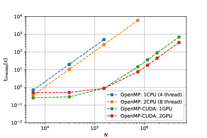


We tested the effectiveness of the different parallelization methods with multiple non-periodic comoving CDM cosmological simulations with different particle numbers in three different hardware settings. The first 10 time steps were timed directly in each case and for further scaling calculations we normalized the wall-clock time with the number of time steps for each simulation. We benchmarked the CPU-only MPI-OpenMP parallelization by running simulations with various particle and node number setups on the Eötvös University (ELTE) Atlasz HPC2009 cluster44 4 https://hpc.iig.elte.hu. Note that this machine cannot be considered as a modern HPC, so rather the relative than the absolute values should be considered in the analysis. On Atlasz HPC2009 each node had two Intel Xeon E5520 CPUs, and OpenMP parallelization was used inside each computing node. For , the communication cost was below 2%, when 16 computing nodes were used. For testing the OpenMP-GPU paralellization, we run our simulations on a single computing node with four Nvidia GeForce GTX 1080 Ti GPUs in the GPU Laboratory of the Hungarian Academy of Sciences, the results can be seen in Fig. 3. Our test simulation with particles achieved times acceleration with just two GPUs with single precision, compared to one Xeon E5520 CPU node, used in the MPI-OpenMP benchmark. We have sustained 9.3Tflop/s on this node, and this is of the theoretical peak performance and roughly of the efficiency of the -GPU direct N-body code[19]. Also, it is clear from this test, that using multiple GPUs is only worth it if the particle number is large enough. Our final test was done on the GPU cluster of the Maryland Advanced Research Computing Center55 5 https://www.marcc.jhu.edu/ (MARCC). The measured timestep wall-clock times as a function of compute nodes can be seen in Fig. 4. Up to 10 compute nodes with 20 Nvidia Tesla K80 dual-GPU cards were used, totalling 40 GPUs. The effectiveness of parallelization turned out to be over 93% for our largest test run with particles for 32 GPUs with 8 MPI tasks, above which the effectiveness started to decline.
| Number of MPI tasks | Efficiency | ||
|---|---|---|---|
| 1 | 5942.11 | 1 | 1.0 |
| 2 | 3060.33 | 1 | 0.97083 |
| 4 | 1524.02 | 1 | 0.97474 |
| 6 | 1042.30 | 2 | 0.95016 |
| 8 | 784.11 | 2 | 0.94727 |
| 12 | 524.20 | 3 | 0.94463 |
| 16 | 388.65 | 4 | 0.95557 |
| 24 | 263.21 | 6 | 0.94065 |
| 32 | 198.10 | 8 | 0.93736 |
| 40 | 169.67 | 10 | 0.87554 |
3 Generating Initial Conditions
The main motivation for running cosmological simulations is to calculate the evolution of statistical properties of the density field over time. To do this, one has to start the simulation from an initial particle distribution at early time with the right correlation function. The statistics of the density field at the epoch of the recombination () is known from the cosmic microwave background measurements[20, 21]. From this point, the power spectrum as a function of wavenumber can be calculated for later times with perturbation theory. Since these analytic methods do not, or not fully take the nonlinear effects into account, perturbative techniques alone are not suitable for calculating the present for small scales, yet they can be used to generate initial conditions (ICs) down to with linear methods and with second order techniques – depending also on mass resolution[22]. In [8], we presented an IC generator algorithm that based on a remapping of an existing periodic initial condition with HEALPix[23] tiling. Because the HEALPix tiling is not perfectly isotropic, the small artificial density fluctuations can grow and cause distortions during the simulation. In the rest of this section we present a new IC generation algorithm for StePS simulations that is free from non-uniformity.
3.1 Generating spherical glasses
The first step of generating the initial conditions is to generate a particle distribution that represents a constant density field, and the net gravitational force acting on each particle is as small as possible. This is a non-trivial problem and it is not clear whether a correct answer even exists[24, 25]. Nevertheless, in case of periodic simulation with translational symmetry, two different solutions are used. The first method places the particles onto a three-dimensional grid, whereas the other solution uses a periodic glass. Using a periodic glass was first suggested by White[26], and it is used in most cosmological N-body simulations nowadays. Glasses are generated by placing point masses randomly in a periodic box, usually smaller than the simulation box itself, and evolving them in an Einstein-de Sitter universe with reversed gravity. Simulations with glassy initial conditions show significantly smaller discreteness artifacts at small scales compared to grid-based ICs. The other advantage of this approach is that glasses are more isotropic.
For a StePS simulation, particle glasses have to be generated with radially decreasing resolution. We start by compactifying the real space using inverse stereographic projection which maps the 3 dimensional Euclidean space onto the 3D hypersurface of a 4D sphere. When Cartesian coordinates are used in the three-dimensional space, the transformation rules for the inverse stereographic projection are
| (14) | ||||
where , and are the angular coordinates on the three-dimensional hypersurface of the four dimensional hypersphere, is the diameter of the hypersphere, and , , are the coordinates in real space. The forward transformations are given by
| (15) | ||||
We note that stereographic projection is only used when generating the initial conditions but all other calculations are done in real space to minimize floating point operations.
To generate initial conditions for StePS simulations with radially decreasing resolution one starts by dividing the compactified space into slices along constant spheres. This is the equivalent of slicing the real space into concentric spherical shells. In every shell we place particles randomly, and transform their coordinates into the real space with eq. 15 stereographic projection. The masses of the particles in the shell with index are
| (16) |
where is the real-space volume of the shell. The increase rate of particle mass with radius depends on the increase rate of volume of real space shells. Depending on the slicing of the compactified space, the increase rate can be controlled. We implemented two slicing schemes.
The first scheme is called “constant binning”, where the compactified space is divided into equally spaced shells along the compact coordinate but, to set a lower limit on particle mass, the innermost shells within an cut-off are united into a single volume with
| (17) |
particles of equal mass, where is the real space radius corresponding to compactified coordinate. Since particle masses vary with radius, the introduction of the cut-off is important and the distinction between the innermost shells and outer shells is necessary to prevent the mixing of particles with too high mass ratios, which would cause artificial distortions in the simulation. The blue curve in Fig. 5 shows the particle mass as a function of radius where the unified innermost shells are visible as the constant line between . The main advantage of the “constant binning” method is that if one chooses large enough, the effect of different mass particle mixing will be minimal at the center.

The other implemented binning method is called the “constant compact space volume” method. In this case we define shells along the compact coordinate such way that the resulting shells have the same compactified volume. The equation for the lower limit of the -th shell in the coordinate is
| (18) |
where is the volume of a bin in the compact space. This equation must be solved numerically for each shell. After the limits for the shells are calculated, we place particles randomly into each shell, and transform the coordinates back to the real space. The particle masses are calculated from Eq. 16 for every shell. With this method the particle masses will decrease smoothly outwards in the entire simulation volume, as it is shown by the red curve in Fig. 5.
Many other realizations of space binnings are possible. Also, one can use different compactification maps or it is possible to change the angular resolution by setting to dependent, etc. We will discuss these possibilities in a future study.
Once the spatial binning is defined and particle coordinates and masses are generated, we follow the standard way of glass generation. By integrating Eq. 8 with reversed gravity, after a sufficiently long relaxation period, the particles will settle down into a glass-like configuration. With the current implementation, glass generation takes a time comparable to running the simulation since in a spherical setting, one cannot use the trick of periodic glass generation with a significantly smaller box than the entire simulation volume. On the other hand, once a glass is generated, it can be reused for generating any number of initial conditions as long as particle number is the same.
We illustrate the generated glasses in Fig. 6 for both, “constant binning” and “constant compact space volume” methods for wedges of cut out of the glasses.


3.2 Perturbing the glass particles
Here we summarize the basic ideas of initial condition generation for periodic simulations, and introduce our new algorithm for the StePS geometry.
The first step is to calculate the power spectrum for the initial time. In linear Eulerian perturbation theory, every mode of the power spectrum is evolving independently, and modes can be scaled to any scale factor via the
| (19) |
growth function[27]. The power spectrum should be normalized at present day scale factor to be consistent with the cosmological parameter. After the initial power spectrum is calculated, the Fourier transform of the density fluctuation field can be generated assuming a Gaussian random field[25]. is calculated in a finite range: from zero to the Nyquist wavenumber in each dimension, which is given by the average particle spacing.
Once the density field is calculated, one only needs to perturb the positions and velocities of the particles to generate the initial conditions. In Lagrangian fluid dynamics, the movement of fluid elements is described by the initial coordinates and the displacement field . The perturbed coordinates become
| (20) |
where is the initial time, and . Lagrangian Perturbation Theory (LPT) uses a perturbative approach to calculate the displacement field from Fourier space density fluctuations [28, 29] in the form of
| (21) |
The first order solution is called the Zel’dovich-approximation[30], which can be written as
| (22) | ||||
| (23) | ||||
| (24) |
where are the initial, and are the final coordinates of the particles. Of course, the displacement field is calculated in a cubic grid, and is interpolated to the original position of the glass particles. Similarly, the second order solution of Lagrange perturbation theory (2LPT)[22] is also used for initial condition generation. In case of periodic initial conditions with constant particle mass, particle masses are calculated directly from Eq. 6.
The IC generation algorithm for our spherically symmetric geometry is very similar but there are two main differences. The first difference is that we do not have a typical average particle spacing in the simulation volume because the mass and the spatial resolution decreases in the radial direction. The second difference is that we do not have a periodic geometry, so we can almost freely choose the box-size in which the fluctuations are calculated by using the Zel’dovich or 2LPT approximation. If one is interested in the effects of simulating sub-survey fluctuations only, should be chosen. In this case, the same density field will be repeated multiple times to cover the simulation sphere. On the other hand, when is chosen, super-survey modes can be simulated, although they will never be resolved and will be prone to cosmic variance due to the large but finite simulated volume. In this case the ICs will be truly non-periodic.
In traditional simulations, the cut-off at large is determined by the average particle separation which is proportional to the cubic root of particle number. In our case, average particle separation is not constant across the simulation volume but grows with the radial distance from the center. As the simplest solution, one can use the Nyquist wavenumber that corresponds to the best resolution at the center of the simulation. When the displacement field is applied to the particle glass, the lower resolution outer parts will undersample the density field which might lead to aliasing effects. In practice, however, these aliasing effects do not seem to affect simulation results. Despite of this, we implemented another method which is from undersampling. This second method works by computing the displacement field with a few different cutoff wavenumbers corresponding to the radius dependent average displacements in spherical shells around the center of the simulation. The actual displacement of the particles is calculated by interpolating between the displacement fields with the nearest cutoffs. To calculate the displacement fields, we relied on the publicly available NgenIC[31] and 2LPTic[32] codes for the Zel’dovich and the 2LPT approximation, respectively.
To be consistent to the desired cosmological parameters, the next step is to set the particle masses to
| (25) |
where is the mass of the th particle, is the original mass of the glass particle, and is the radius of the simulation. If the goal is to generate ICs for a non-comoving simulation, one last step should be taken: rescaling the coordinates and adding the Hubble flow to velocities.
4 Demonstration of the method
For illustration, we aimed to re-simulate the Millennium Run[12] with the StePS code. The Millennium Simulation had a great impact and demonstrated the effectiveness of the GADGET cosmological tree code. The original simulation had particles in a periodic cube of linear size. It used 512 processors and required about 28 days of wall-clock time on an IBM p690 supercomputer.
We used the same cosmological parameters and random seed to generate the initial conditions for the non-periodic StePS simulation. The radius of the simulation was set to , and we used constant binning, c.f. Sec. 3. The radius of the inner, constant resolution sphere around the simulation center was Mpc. The spatial resolution at the center was times worse than the original Millennium Simulation. Our simulation ran for 106 wall-clock hours on 12 Nvidia GeForce 1080ti GPUs. The parameters of both simulations are summarized in Table 2.
| Millennium | StePS | |
|---|---|---|
| Initial redshift | ||
| linear size | ||
| simulated volume | ||
| number of particles | ||
| particle mass | - | |
| force calculation | ||
| memory use | ||
| number of processing units | (CPU) | (GPU) |
| wall-clock time | ||
4.1 Results
To compare the constant resolution Millennium Simulation to StePS , we compactified the snapshot of the original Millennium Run by placing multiple copies of the simulation cube side by side and applying Eq. 14. We aggregated the particles with constant binning in the radial direction and with equal-area HEALPix[23] tiling in the and coordinates. We averaged the positions, summed up the masses and inertia of the dark matter particles in each bin and substituted them with a single particle. After decompactification with Eq. 15, we arrived at a particle distribution with a very similar resolution to the StePS simulation as a function of radius. The comparison of Millennium and the StePS simulation can be seen in Fig. 7 at different scales. While the Millennium Simulation has slightly better resolution the the StePS simulation at the very center (see the top panels of Fig. 7), the structure at are identical. Some differences between Millennium and StePS are visible at large distances from the center (see the bottom panels of Fig. 7): structures in the StePS simulation are sharper at large radii. This is due to the fact that compactification and time evolution are not interchangeable operations.


5 Summary
We presented a multi-GPU implementation of the StePS code, and demonstrated the effectiveness of parallelization. We also implemented a new initial condition generator for compactified simulations. We were able to reproduce the Millennium Simulation at a spatial resolution slightly worse than the original at the very center of the StePS simulations on 12 GPUs in under 106 hours. The source code of the simulation program and the IC generator script is freely available at our github repository (https://github.com/eltevo/StePS), licensed under GNU General Public License v2.0.
Acknowledgements
The authors would like to thank Volker Springel and Adrian Jenkins for helping recreate the Millennium initial conditions. We also want to thank Robert Beck for stimulating discussions. This work has been supported by the NKFI grants NN 114560 and NN 129148. IS acknowledges support from National Science Foundation (NSF) award 1616974. We would like to thank the GPU Laboratory of the Hungarian Academy of Sciences, Wigner Research Centre of Physics for providing computing resources. Part of this research project was conducted using the computational resources at the Maryland Advanced Research Computing Center (MARCC).
References
- [1] V. Springel, The cosmological simulation code GADGET-2, MNRAS364 (2005) 1105–1134. arXiv:astro-ph/0505010, doi:10.1111/j.1365-2966.2005.09655.x.
- [2] J. F. Navarro, C. S. Frenk, S. D. M. White, The Structure of Cold Dark Matter Halos, ApJ462 (1996) 563. arXiv:astro-ph/9508025, doi:10.1086/177173.
- [3] W. H. Press, P. Schechter, Formation of Galaxies and Clusters of Galaxies by Self-Similar Gravitational Condensation, ApJ187 (1974) 425–438. doi:10.1086/152650.
- [4] D. Potter, J. Stadel, R. Teyssier, PKDGRAV3: beyond trillion particle cosmological simulations for the next era of galaxy surveys, Computational Astrophysics and Cosmology 4 (2017) 2. arXiv:1609.08621, doi:10.1186/s40668-017-0021-1.
- [5] A. W. Appel, An Efficient Program for Many-Body Simulation, SIAM Journal on Scientific and Statistical Computing, vol. 6, no. 1, January 1985, p. 85-103. 6 (1985) 85–103.
- [6] J. Barnes, P. Hut, A hierarchical O(N log N) force-calculation algorithm, Nature324 (1986) 446–449. doi:10.1038/324446a0.
- [7] A. A. Klypin, S. F. Shandarin, Three-dimensional numerical model of the formation of large-scale structure in the Universe, MNRAS204 (1983) 891–907. doi:10.1093/mnras/204.3.891.
- [8] G. Rácz, I. Szapudi, I. Csabai, L. Dobos, Compactified cosmological simulations of the infinite universe, MNRAS477 (2018) 1949–1957. arXiv:1711.04959, doi:10.1093/mnras/sty695.
- [9] K. Nitadori, S. J. Aarseth, Accelerating NBODY6 with graphics processing units, MNRAS424 (2012) 545–552. arXiv:1205.1222, doi:10.1111/j.1365-2966.2012.21227.x.
- [10]
M. B. N. Kouwenhoven, L. Wang, R. Spurzem, P. Berczik, S. Aarseth, K. Nitadori,
T. Naab, nbody6++gpu: ready
for the gravitational million-body problem, Monthly Notices of the Royal
Astronomical Society 450 (4) (2015) 4070–4080.
arXiv:http://oup.prod.sis.lan/mnras/article-pdf/450/4/4070/5782448/stv817.pdf,
doi:10.1093/mnras/stv817.
URL https://dx.doi.org/10.1093/mnras/stv817 - [11] P. Berczik, K. Nitadori, S. Zhong, R. Spurzem, T. Hamada, X. Wang, I. Berentzen, A. Veles, W. Ge, High performance massively parallel direct N-body simulations on large GPU clusters., in: International conference on High Performance Computing, Kyiv, Ukraine, October 8-10, 2011., p. 8-18, 2011, pp. 8–18.
- [12] V. Springel, S. D. M. White, A. Jenkins, C. S. Frenk, N. Yoshida, L. Gao, J. Navarro, R. Thacker, D. Croton, J. Helly, J. A. Peacock, S. Cole, P. Thomas, H. Couchman, A. Evrard, J. Colberg, F. Pearce, Simulations of the formation, evolution and clustering of galaxies and quasars, Nature435 (2005) 629–636. arXiv:astro-ph/0504097, doi:10.1038/nature03597.
- [13] J. F. Navarro, S. D. M. White, Simulations of dissipative galaxy formation in hierarchically clustering universes-2. Dynamics of the baryonic component in galactic haloes, MNRAS267 (1994) 401–412. doi:10.1093/mnras/267.2.401.
- [14] C. Power, J. F. Navarro, A. Jenkins, C. S. Frenk, S. D. M. White, V. Springel, J. Stadel, T. Quinn, The inner structure of CDM haloes - I. A numerical convergence study, MNRAS338 (2003) 14–34. arXiv:astro-ph/0201544, doi:10.1046/j.1365-8711.2003.05925.x.
- [15] J. J. Monaghan, J. C. Lattanzio, A refined particle method for astrophysical problems, A&A149 (1985) 135–143.
- [16] P. P. Ewald, Die Berechnung optischer und elektrostatischer Gitterpotentiale, Annalen der Physik 369 (1921) 253–287. doi:10.1002/andp.19213690304.
- [17] L. Hernquist, F. R. Bouchet, Y. Suto, Application of the Ewald method to cosmological N-body simulations, ApJS75 (1991) 231–240. doi:10.1086/191530.
- [18] T. Quinn, N. Katz, J. Stadel, G. Lake, Time stepping N-body simulations, ArXiv Astrophysics e-printsarXiv:astro-ph/9710043.
- [19] P. Berczik, R. Spurzem, L. Wang, S. Zhong, O. Veles, I. Zinchenko, S. Huang, M. Tsai, G. Kennedy, S. Li, L. Naso, C. Li, Up to 700k gpu cores, kepler, and the exascale future for simulations of star clusters around black holes.
- [20] C. L. Bennett, D. Larson, J. L. Weiland, N. Jarosik, G. Hinshaw, N. Odegard, K. M. Smith, R. S. Hill, B. Gold, M. Halpern, E. Komatsu, M. R. Nolta, L. Page, D. N. Spergel, E. Wollack, J. Dunkley, A. Kogut, M. Limon, S. S. Meyer, G. S. Tucker, E. L. Wright, Nine-year Wilkinson Microwave Anisotropy Probe (WMAP) Observations: Final Maps and Results, ApJS208 (2013) 20. arXiv:1212.5225, doi:10.1088/0067-0049/208/2/20.
- [21] Planck Collaboration, N. Aghanim, Y. Akrami, M. Ashdown, J. Aumont, C. Baccigalupi, M. Ballardini, A. J. Banday, R. B. Barreiro, N. Bartolo, S. Basak, R. Battye, K. Benabed, J.-P. Bernard, M. Bersanelli, P. Bielewicz, J. J. Bock, J. R. Bond, J. Borrill, F. R. Bouchet, F. Boulanger, M. Bucher, C. Burigana, R. C. Butler, E. Calabrese, J.-F. Cardoso, J. Carron, A. Challinor, H. C. Chiang, J. Chluba, L. P. L. Colombo, C. Combet, D. Contreras, B. P. Crill, F. Cuttaia, P. de Bernardis, G. de Zotti, J. Delabrouille, J.-M. Delouis, E. Di Valentino, J. M. Diego, O. Doré, M. Douspis, A. Ducout, X. Dupac, S. Dusini, G. Efstathiou, F. Elsner, T. A. Enßlin, H. K. Eriksen, Y. Fantaye, M. Farhang, J. Fergusson, R. Fernandez-Cobos, F. Finelli, F. Forastieri, M. Frailis, E. Franceschi, A. Frolov, S. Galeotta, S. Galli, K. Ganga, R. T. Génova-Santos, M. Gerbino, T. Ghosh, J. González-Nuevo, K. M. Górski, S. Gratton, A. Gruppuso, J. E. Gudmundsson, J. Hamann, W. Handley, D. Herranz, E. Hivon, Z. Huang, A. H. Jaffe, W. C. Jones, A. Karakci, E. Keihänen, R. Keskitalo, K. Kiiveri, J. Kim, T. S. Kisner, L. Knox, N. Krachmalnicoff, M. Kunz, H. Kurki-Suonio, G. Lagache, J.-M. Lamarre, A. Lasenby, M. Lattanzi, C. R. Lawrence, M. Le Jeune, P. Lemos, J. Lesgourgues, F. Levrier, A. Lewis, M. Liguori, P. B. Lilje, M. Lilley, V. Lindholm, M. López-Caniego, P. M. Lubin, Y.-Z. Ma, J. F. Macías-Pérez, G. Maggio, D. Maino, N. Mandolesi, A. Mangilli, A. Marcos-Caballero, M. Maris, P. G. Martin, M. Martinelli, E. Martínez-González, S. Matarrese, N. Mauri, J. D. McEwen, P. R. Meinhold, A. Melchiorri, A. Mennella, M. Migliaccio, M. Millea, S. Mitra, M.-A. Miville-Deschênes, D. Molinari, L. Montier, G. Morgante, A. Moss, P. Natoli, H. U. Nørgaard-Nielsen, L. Pagano, D. Paoletti, B. Partridge, G. Patanchon, H. V. Peiris, F. Perrotta, V. Pettorino, F. Piacentini, L. Polastri, G. Polenta, J.-L. Puget, J. P. Rachen, M. Reinecke, M. Remazeilles, A. Renzi, G. Rocha, C. Rosset, G. Roudier, J. A. Rubiño-Martín, B. Ruiz-Granados, L. Salvati, M. Sandri, M. Savelainen, D. Scott, E. P. S. Shellard, C. Sirignano, G. Sirri, L. D. Spencer, R. Sunyaev, A.-S. Suur-Uski, J. A. Tauber, D. Tavagnacco, M. Tenti, L. Toffolatti, M. Tomasi, T. Trombetti, L. Valenziano, J. Valiviita, B. Van Tent, L. Vibert, P. Vielva, F. Villa, N. Vittorio, B. D. Wandelt, I. K. Wehus, M. White, S. D. M. White, A. Zacchei, A. Zonca, Planck 2018 results. VI. Cosmological parameters, ArXiv e-printsarXiv:1807.06209.
- [22] M. Crocce, S. Pueblas, R. Scoccimarro, Transients from initial conditions in cosmological simulations, MNRAS373 (2006) 369–381. arXiv:astro-ph/0606505, doi:10.1111/j.1365-2966.2006.11040.x.
- [23] K. M. Górski, E. Hivon, A. J. Banday, B. D. Wandelt, F. K. Hansen, M. Reinecke, M. Bartelmann, HEALPix: A Framework for High-Resolution Discretization and Fast Analysis of Data Distributed on the Sphere, ApJ622 (2005) 759–771. arXiv:astro-ph/0409513, doi:10.1086/427976.
- [24] L. Hernquist, N. Katz, TREESPH - A unification of SPH with the hierarchical tree method, ApJS70 (1989) 419–446. doi:10.1086/191344.
- [25] E. Sirko, Initial Conditions to Cosmological N-Body Simulations, or, How to Run an Ensemble of Simulations, ApJ634 (2005) 728–743. arXiv:astro-ph/0503106, doi:10.1086/497090.
- [26] S. D. M. White, Formation and Evolution of Galaxies: Les Houches Lectures, ArXiv Astrophysics e-printsarXiv:astro-ph/9410043.
- [27] S. Dodelson, Modern cosmology, Academic Press, 2003.
- [28] I. B. Zeldovich, The theory of the large scale structure of the universe, in: M. S. Longair, J. Einasto (Eds.), Large Scale Structures in the Universe, Vol. 79 of IAU Symposium, 1978, pp. 409–420.
- [29] M. White, The Zel’dovich approximation, MNRAS439 (2014) 3630–3640. arXiv:1401.5466, doi:10.1093/mnras/stu209.
- [30] Y. B. Zel’dovich, Gravitational instability: An approximate theory for large density perturbations., A&A5 (1970) 84–89.
- [31] V. Springel, NGenIC: Cosmological structure initial conditions, Astrophysics Source Code Library (Feb. 2015). arXiv:1502.003.
- [32] M. Crocce, S. Pueblas, R. Scoccimarro, 2LPTIC: 2nd-order Lagrangian Perturbation Theory Initial Conditions, Astrophysics Source Code Library (Jan. 2012). arXiv:1201.005.