Koopman-Based Approach to Non-intrusive Projection-Based Reduced-Order Modeling with Black-Box High-Fidelity Models. Part II: Application Submitted to the editors

The total number of observables, $O$ is essentially inifinite if one were seeking a closed linear transformation of the non-linear FOM [10]. However we seek to find a finite $O$ which might result in an un-closed linear transformation which are then closed with a set of constraints. In this work, $O$ represents the total number of terms in the FOM that are functions of the state and are operated by a linear differential operator; each of the $g_{i}(\mathbf{u})$’s is picked from knowledge of the FOM in its continuous PDE form, as will be illustrated in section 3. For a FOM that is a system of $S$ coupled PDEs, note that $O\geq S$ always and $O>S$ for a non-linear system. Therefore the observables can be written

Finally, to close the under-determined transformed system, we add algebraic equations that establish the non-linear consistency relationship between the observables and the state thereby providing closure. These constraints are of the form

where, $f_{i}:\mathbb{R}^{N}\rightarrow\mathbb{R}^{N}$ is a function that operates on the observables. Note that for a system of $S$ coupled PDEs, $O-S$ constraints are needed to be specified to achieve closure. Although, there is no unique way of specifying these constraints, we provide some guidelines in section 2.1. Equation (6) along with (4) together form a closed system upon which model reduction is performed. To perform the projection, the truncated basis set for each observable $\mathbf{y}_{i}$ is extracted by performing POD on the snapshot matrix of $\mathbf{y}_{i}$ (generated by running the FOM at $M$ distinct parameter points) and are denoted $\Phi_{i}\in\mathbb{R}^{N\times k_{i}}$, i.e.

where $\mathbf{y}_{i}^{(j)}$ is the $jth$ snapshot of observable $\mathbf{y}_{i}$, $\Phi_{i}$ is the first $k_{i}$ columns of $\mathbf{V}_{i}$, $M$ is the total number of snapshots used for model training and the POD basis vectors are obtained from the thin-svd decomposition of $\mathbf{Y}_{i}$. This leads to the trial basis matrix for the overall system defined as a block-diagonal matrix of all the $O$ POD basis set given below

where $k=k_{1}+\ldots+k_{O}$. The reduced observable is then given by $\tilde{\mathbf{y}}_{i}\approx\Phi_{i}^{\top}\mathbf{y}_{i}$. Recall that $\mathbf{A}$ is non-square since it is $\in\mathbb{R}^{N\times ON}$, and hence a suitable choice for the test basis for projection is $\mathbf{\Psi}=\mathbf{A}\mathbf{\Phi}$. Note that this choice of the test basis is equivalent to a galerkin projection ($\mathbf{\Psi}=\mathbf{\Phi}$) on the normal equations. i.e. on $\mathbf{A}^{\top}\mathbf{A}\mathbf{y}=\mathbf{A}^{\top}\mathbf{f}$. Let $\mathbf{B}=\mathbf{A}^{\top}\mathbf{A}\in\mathbb{R}^{ON\times ON}$; then the projection leads to

Setting $\tilde{\mathbf{f}}=\mathbf{\Phi}^{\top}\mathbf{A}^{\top}\mathbf{f}\in\mathbb{R}^{k}$ and $\tilde{\mathbf{B}}=\mathbf{\Phi}^{\top}\mathbf{B}\mathbf{\Phi}\in\mathbb{R}^{k\times k}$, this leads to the reduced order model

The ROM given by Equation 10 is now a $k\times k$ system where $k<<N$ and is solved along with the constraints presented in Equation 6, posed as a non-linear program as shown below

The main hypothesis of this work is that the ROM given by Equation 11 still approximately satisfies the governing equations and this is verified in the Section 4. The optimization problem in Equation 11 needs special treatment to handle the non-linear constraints which still depend on the full state of observables, and is efficiently done using the DEIM  [13]; see Appendix 7.3 for details on implementation for a specific example. The ROM in (11) is solved via Sequential Quadratic Programming (SQP) [14] with the objective function and constraint tolerances set to $10^{-6}$ and the number of function evaluations bounded by $4\times 10^{6}$. The initial guess to the solution of (11) is given as the nearest flow snapshot to the test parameter at which prediction is sought.

The proposed approach that leads to the ROM in the form of (10) corresponds to one parameter snapshot since $\tilde{\mathbf{B}}$ and $\tilde{\mathbf{f}}$ are parameter dependent. Therefore, the approach generates a database of ROMs for a pre-determined set of parameter snapshots, which are later interpolated to predict the state at a new parameter. The interpolation is carried out in a manner that retains the inherent structure and properties of the matrix $\mathbf{\tilde{B}}$ post-interpolation. The general principle that is followed is to map the matrices to a plane that is locally tangent to the manifold in which they are originally embedded. The anchor point on the manifold, which is the point of tangency is chosen to be one of the matrices themselves. While this choice is arbitrary, in this work we use the matrix that corresponds to the nearest (in the standardized Euclidean sense) parameter snapshot to the test parameter. The traditional Euclidean space interpolation (where typical vector operations are valid) is then carried out in the tangent plane after which they are mapped back to the manifold. The mapping to and from the tangent plane are carried out via logarithmic and exponential relationships as depicted in Figure 2.

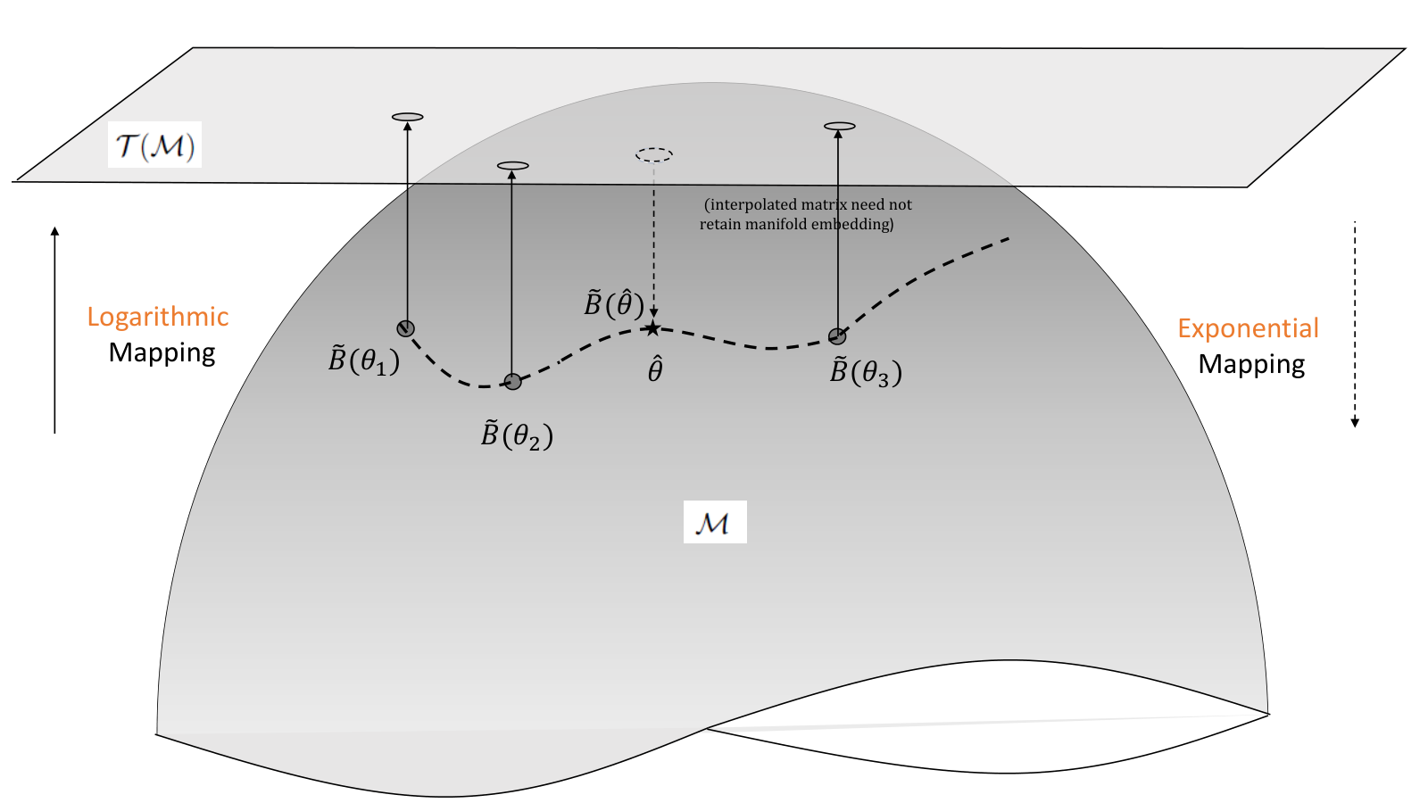
The matrix $\tilde{\mathbf{B}}=\mathbf{\Phi}^{\top}\mathbf{A}^{\top}\mathbf{A}\mathbf{\Phi}$ in Equation 11 is symmetric positive definite (SPD) for the following reasons. Firstly, $\mathbf{A}^{\top}\mathbf{A}$ is a co-variance matrix and hence is symmetric positive semi-definite (see [15], sec. 5.3 ). Furthermore, multiplication by orthogonal matrix $\mathbf{\Phi}$ of rank $k$ where $k<rank(A)$ ensures $\tilde{\mathbf{B}}$ is SPD. SPD matrices of size $k\times k$ form a special group called the $SPD(k)$  [16, 17] and the manifold they are embedded in is denoted as $\mathcal{M}$. Also, for the set of all SPD matrices $\mathbf{B}~\in\mathcal{M}$, the tangent plane is the set of all symmetric matrices, $\mathbf{B^{\prime}}$  [17]. Any metric ($\mathcal{M}_{f}$) defined on $SPD(k)$ for any two matrices uses the following functional relationship

which leads to the following results for the exponential and logarithmic mapping for $SPD(k)$ [16] where, $\tilde{\mathbf{B}}_{0}$ is the anchor point and $\tilde{\mathbf{B}^{\prime}}$ is the point whose mapping is desired. The exponential mapping of $\tilde{\mathbf{B}}^{\prime}$ from tangent plane to $\mathcal{M}$ at $\tilde{\mathbf{B}}_{0}\in\mathcal{M}$, to $\mathcal{M}$ is given by

and the logarithmic mapping of $\tilde{\mathbf{B}}\in\mathcal{M}$ to tangent plane to $\mathcal{M}$ at $\tilde{\mathbf{B}}_{0}\in\mathcal{M}$:

The results presented in Equations 13 and 14 are used in this work to perform mapping to and from the tangent space. Once on the tangent space the matrices are interpolated element-wise using multivariate Lagrange polynomials of $2^{nd}$ order. The overall method is summarized in Figure 3.

The Euler equations governing the 2D, compressible, inviscid flow past an airfoil are the governing equations on which we perform model reduction. This coupled non-linear system is solved via the commercial black-box CFD solver, STARCCM+ [18]. The equations in conservation form is provided in Eq.15 below,

where

and $\nabla_{x}$ and $\nabla_{y}$ are the $x$ and $y$ components of the gradient operator $\nabla$ respectively. The following transformation is then performed

from the state variables to observables, leading to the lifted model.

where in the above equation, empty spaces in the matrix denote zeros. The equation upon discretization leads to

where, $\mathbf{G}_{x}$ and $\mathbf{G}_{y}$ represents the discrete version of the gradient operators $\nabla_{x}$ and $\nabla_{y}$ respectively and the empty spaces denote block matrices of zeros. The parameter-dependent $\mathbf{A}$ matrix is obtained directly by discretizing the linear terms $\mathbf{G}_{x}$ and $\mathbf{G}_{y}$ via finite volume method. The grid is exported in the CFD General Notation System (CGNS) [19] for this purpose, as mentioned in Figure 3. The snapshots $\mathbf{y}$ are applied to the $\mathbf{A}$ matrix and the RHS $\mathbf{f}$ is extracted for each parameter. With the FOM reduced to the $\mathbf{A}\mathbf{y}=\mathbf{f}$ form and $\mathbf{A}\in\mathbb{R}^{4N\times 8N},~\mathbf{y},\mathbf{f}\in\mathbb{R}^{8N}$, Equation 17 represents an under-determined system. Therefore they are closed using non-linear constraints given by Equation 18. Notice that the constraints express the relationship between the first $S=4$ observables ($y_{1}$ through $y_{4}$) and the remaining $O-S;~(O=8)$ observables ($y_{5}$ through $y_{8}$). As mentioned in the previous section, the choice of the first $S$ observables and hence the $O-S$ constraints is non-unique. However, from experience trying out different choices in this work, it is found that the following heuristics ensure a stable transformation from the observables back to the state: (i) the terms starting from the lowest order are picked as the first $S$ observables ($\rho u,\rho v,\rho uv,p$ in this case) and (ii) one of the first $S$ observables is set to be a state variable ($y_{4}=p$ in this case). It should be noted that all the observables that are in excess of the number of equations can be expressed as some function of the rest because the number of independent observables are only as many as the number of PDEs in the FOM ($S=4$). The constraints are expressed in terms of the continuous form of the state and observable as follows

With discrete observables ($\mathbf{y}_{i}$) all the operations in (15) are performed element-wise. In all the results presented in the following sections, the POD modes constituting $99.99\%$ of the energy (cumulative fraction sum of the singular values in $\mathbf{\Sigma}_{i}$) are retained. The error metrics used for all the results are defined as follows

The baseline shapes are parameterized using Class Shape Transformation (CST) [20, 21]. The CST model of parametrization defines a class function $c$ and a shape function $s$ and the curve being parameterized is specified as their product. The main idea is that the class function serves to define a general class of geometry such as airfoils, missiles or sears-haack body, while the shape function serves to define the unique shape within a particular class of shapes (such as a NACA0012 vs RAE2822 airfoil). The class function, $c(\psi)$ is more generally defined as

where the variable $\psi$ represents the non-dimensional chord-wise distance. $n_{1}$ and $n_{2}$ define the specific class; for instance $n_{1}=0.5,~n_{2}=1$ and hence $\sqrt{\psi}(1-\psi)$ defines airfoils with rounded leading edge and a sharp trailing edge [20]. The unique shape of an airfoil is driven by the shape function, specified as follows

where $A_{i}$ are the coefficients which are also the shape parameters. The NACA0012 and RAE2822 are parameterized using 6 and 8 variables respectively, whose values are given by $A_{NACA0012}$ and $A_{RAE2822}$ where the top and bottom rows correspond to the upper and lower surfaces of the airfoils. Further details of the parameterization are provided in Appendix 7.1.

The CST coefficients representing the NACA0012 baseline is perturbed $\pm$ 30% to generate new airfoil shapes, a sample of which is shown in Figure 5. A total of 170 such points were generated using a Latin Hypercube design, $M=$160 of which was used in model building while the remaining was used to validate the model. The system matrix $\tilde{\mathbf{B}}$ is interpolated in the tangent space to the manifold of symmetric positive definite matrices, as explained in Section 2.2, while the RHS $\tilde{\mathbf{f}}$ is interpolated in the Euclidean space. In both cases a multi-variate polynomial in the Lagrange form is used for interpolation as mentioned previously (see Renganathan(2018) [11], Algorithm 1 for details).

The comparison of the ROM predicted pressure coefficient on the airfoil surface against the FOM solution, for a select two of the validation set is shown in Figure 6. Across all the 10 validation cases, the maximum and average errors in $C_{P}$ are $\approx$ 5% and $\approx$ 2% respectively, whereas the computational speedup is $\approx$ 100x. Therefore, the effectiveness of proposed approach is well established. Similar accuracy was observed with the lift coefficient, which are tabulated in Appendix 7.2. The overall flow-field comparison in terms of overlaid pressure and mach number contours is also shown in Figure 6 which further re-iterate the low prediction errors observed.

Now we demonstrate the method in the transonic regime using the RAE2822 test case. Similar to the NACA test case, CST coefficients representing the baseline are perturbed $\pm$ 30 % to generate new airfoil shapes, a sample of which is shown in Figure 7. A total $M=$160 snapshots were again used in model building. However, the freestream mach number for this case is set as $\mathbb{M}=0.734$ which leads to a shock whose strength and location are affected by perturbing the shape CST coefficients. The rest of the freestream conditions are summarized in Table 2

We begin by comparing the ROM predictions against FOM solutions in terms of the coefficient of pressure distributions in Figure 8. Two specific cases are showcased in the figure to illustrate the strength and weakness of the approach in transonic regime. Overall, from all the validation cases, it is observed that the ROM does capture the shock location within a maximum error of 5%. However, this translates in to an average $L_{2}$ error of 8.5% in $C_{P}$ predictions and about 16% in the prediction of $C_{d}$. The average error in $C_{l}$ predictions were much lower at 4%. Such a trend where the lift coefficient were predicted with greater accuracy than drag was also previously observed in [1]. The main reason for this is expected to be that in the absence of viscous effects, the computation of the drag force shows greater sensitivity to discrepancy in pressure. This is because unless at high angles of attack, the projected area in the direction normal to the freestream velocity is very small leading to larger sensitivities in $C_{d}$ computations. However, as will be demonstrated in section 5.3, the proposed approach demonstrates more robustness in the drag prediction than competing methods.

Under subsonic shock-free conditions, the predictions are consistently under 5% whereas under transonic conditions, the predictive capability drops. In the presence of discontinuities in the flow field such as moving shocks, a POD-based method is unable to accurately predict shock location and strength. Such a limitation has been reported by others in the literature who propose a domain-decomposition method to isolate the shock-prone regions of the flow-field where the FOM is solved whereas the ROM is used to approximate the rest of the flow field [22, 23]. However such methods are intrusive in the sense that they might require access to source code of the FOM to effectively manipulate the flow domains which is not feasible with black-box codes. Another method reported in the literature to address this problem is to do a space-transformation of the snapshots containing moving discontinuities [24]. The goal of the proposed approach are first steps towards enabling projection-based MOR for black-box static parametric systems although such enhancements can be added to it to address specific problems. Additionally, the solution to the ROM in (10) shows sensitivity to initial guess and hence can lead to a local optimum which also contributes to the performance penalty of the approach in transonic regime. Despite the limitations in the transonic regime, it has been observed that the ROM still predicts the shock within 5% chord-length variability. Furthermore, the $C_{P}$, $C_{d}$ and $C_{l}$ are predicted with an average error of $14\%$, $16\%$ and $4\%$ respectively which are still useful in the conceptual and preliminary stages of the design process where some accuracy can be traded for larger gain in computational costs for faster decision making.

Recall from section 2 that the full and reduced observable are related via the relationship $\tilde{\mathbf{y}}_{i}\approx\mathbf{\Phi}^{\top}\mathbf{y}_{i}$. Here each element of the reduced observable $\tilde{\mathbf{y}}_{i}$ is assumed to be a smooth function of the parameters $\boldsymbol{\theta}$ and is interpolated in the $\boldsymbol{\theta}$-space via Kriging. The Kriging approach assumes that the true response is a relaization of a Gaussian process (GP) which is completely specified by a mean and covariance function and estimates the hyperparameters of the GP from observations at finite number of locations. Kriging interpolates noise-free data, regresses noisy data and the prediction at unknown sites is given by a Gaussian probability distribution as opposed to a deterministic value. However it is customary to use the expected value of the predictive distribution as a surrogate for the true function.

The $jth$ element of the $ith$ reduced observable is assumed to take the form

where $z(\boldsymbol{\theta})\sim\mathcal{N}(\mathbf{0},\mathbf{C})$ with $\mathbf{0}$ being a vector of zeros of appropriate length, $\mathbf{C}$ the covariance matrix and $\mu$ the unknown mean. The GP is assumed to be statistically stationary [29] with homoscedastic variance which simplifies the covariance matrix as $\mathbf{C}_{ij}=\sigma^{2}\mathbf{R}_{ij}$, where $\mathbf{R}$ is the correlation matrix. The assumption of stationarity also means that $\mathbf{R}_{ij}=\mathbf{R}(\|\boldsymbol{\theta}_{i}-\boldsymbol{\theta}_{j}\|)$ where $\|\cdot\|$ denotes the Euclidean distance. The elements of the correlation matrix are defined by a parametrized kernel as $\mathbf{R}_{ij}=r(\boldsymbol{\theta}_{i},\boldsymbol{\theta}_{j}~;\ell)$. The hyperparameters of the Kriging model are therefore $\{\ell,\mu,\sigma^{2}\}$. In this work, we assume the stationary and isotropic squared-exponential kernel are given by the following equation

The training data for each $\tilde{y}_{ij}$ is the $jth$ row of the product $\mathbf{\Sigma}_{i}\times\mathbf{W}_{i}^{\top}$ in the thin-svd step in  (7); let that be denoted as $\tilde{\mathbf{y}}^{j}$. Each $\tilde{\mathbf{y}}^{j}$ is a vector of length $M$ corresponding to the parameter snapshots $\boldsymbol{\Theta}=[\boldsymbol{\theta}_{1},\ldots,\boldsymbol{\theta}_{M}]$. Then the Kriging model assumes that the prediction at some unknown $\boldsymbol{\theta}^{*}$ forms a joint normal distribution with $\tilde{\mathbf{y}}^{j}$. That is

Conditioning the distribution of $\tilde{y}_{ij}^{*}$ in (25) on the observations one then obtains the posterior predictive distribution [28] given by

where $r(\boldsymbol{\theta}^{*},\boldsymbol{\Theta})=r(\boldsymbol{\Theta},\boldsymbol{\theta}^{*})^{\top}$ is a column vector of the correlation between $\boldsymbol{\theta}^{*}$ and $\boldsymbol{\Theta}$ and the unknown mean $\mu=r(\boldsymbol{\theta}^{*},\boldsymbol{\Theta})\mathbf{R}^{-1}\tilde{\mathbf{y}}^{j}$ (which is also our Kriging predictor). The other two hyperparameters ($\ell,\sigma^{2}$) are determined by maximizing the log marginal likelihood of $\tilde{y}_{ij}*$

In aerodynamic design, a specific aerodynamic load distribution about an aerodynamic object is of interest. For instance, under incompressible flow assmptions for a finite wing, an elliptic lift distribution along the wing is known to produce the least induced drag [30]. Similarly, in the preliminary design of propellers [31] and turbines[32], a certain lift distribution along the blade is an input to the design process. In such cases the actual design (shape) parameters that produce such a load distribution is of interest. We call such a problem the inverse design. Here we fix the desired pressure coefficient distribution as our target and search the design space for the shape parameters that would best approximate the target. Then the predicted airfoil shape is compared against the true shape. Therefore we are interested in solving the following optimization problem

where $C^{*}_{P}$ is the target pressure distribution and $R$ is the residual operator. Naturally we want to replace the full-order governing equations with the ROM and hence we solve the modified problem

The free-stream conditions used for this test case are summarized in Table 3. The optimum shape was searched using a GA based optimizer with a population size of 30 per generation and a total of 60 generations. The constraint and function convergence tolerance were set to $10^{-5}$ and $10^{-3}$ respectively and the optimization required a total of 1830 function evaluations to determine the final design. The final design is shown in Figure 9. The predictions by the proposed approach appears quite similar to the POD-Krig. However, the difference is more noticeable in the GA optimizer convergence history shown in Figure 10 where the POD-Krig. leads to a sub-optimal design compared to the proposed approach. In this specific example the proposed approach only marginally outperforms the baseline approach, but this is put to test further in predicting the lift and drag coefficients section 5.3. It was earlier shown in [1] that in the transonic regime a POD-Krig. like approach is prone to predicting non-physical shock patterns mainly because the reduced state is not necessarily smoothly varying. However, such an approach is still effective if the flow does not contain parameter-dependent discontinuities as demonstrated in this example. The main benefit of the proposed approach is the gain in computational times. It required approximately 3.7 hrs of wall-clock time for the inverse design problem whereas the equivalent FOM wall-clock time for the same number of function evaluations is expected to take roughly 300 hrs.

Next, we demonstrate the present methodology towards the uncertainty quantification problem. Uncertainty in aerospace design is inevitable and manifests itself either due to lack of knowledge (ex: biased models) or variability inherent in the system (ex: noisy manufacturing process). The aerospace design process should therefore account for the uncertainties in order to make reliable decisions early on in the design process. Specifically, we are interested in quantifying the uncertainty in the airfoil lift and drag coefficients due to the manufacturing process induced variations in the airfoil shape. We use the same $\pm~30\%$ variation in the airfoil CST coefficients and uniformly sample this design space. A Monte Carlo (MC) [33] simulation is carried out to propagate the input uncertainty into the model to quantify the uncertainties in the quantities of interest - namely, the lift and drag coefficients. We use the NACA test case under operating conditions defined in Table 3.

A total of 4000 samples were uniformly sampled from the $\pm~30\%$ range on the CST coefficients on which the proposed approach (POD-Proj.) and the baseline approach (POD-Krig.) are compared. The FOM is also evaluated at the same set of points in order to provide a reference for comparison. The probability density function is approximated from the 4000 samples via the kernel density estimation (KDE) method [34, 35] with 100 equally-spaced points and a band-width of $0.001$ and $0.017$ for $C_{d}$ and $C_{l}$ respectively. The density plots are shown in Figure 11. In predicting the density plot for $C_{l}$ the two methods perform quite equally. However for $C_{d}$, the proposed approach clearly outperforms POD-Krig. As discussed briefly in section 7.2, this is mainly because the $C_{d}$ shows greater sensitivity to $C_{P}$ distributions compared to $C_{l}$ particularly in 2-D inviscid simulations and hence even modest error in predicting $C_{P}$ can translate into larger errors in $C_{d}$. Secondly, the POD-Krig. approach does not account for the physics of the system unlike the proposed approach and hence performs poorly when the Kriging interpolator does not learn the behavior of the POD coefficients in the parameter space very well. It should be noted that there are other ways to improve upon the Kriging prediction, for instance via using a non-stationary kernel  [36, 28] to capture the underlying correlation in the data. Such models might come with a higher dimensional parametrization but have the potential to emulate rapidly varying non-linear responses very well. However, in the present work the goal is only to make a very general comparison of the proposed approach with a very basic alternative method that is applicable for non-intrusive ROM methods. The statistical measures that quantify the shape of the density plots is summarized in Table 4. As revealed by the table, the statistics for the proposed POD-Proj. approach matches the stats predicted from the FOM much better than the POD-Krig approach.

Another important aspect for discussion are the computational times required for each of the methods. All surrogate model computations were run in serial mode on a desktop computer with 4 cores and 16GB RAM. The ROM computations for 4000 samples consumed approximately 7.2 hrs of wall-clock time whereas the POD-Krig. approach consumed approximately 6.5 hrs. An equivalent budget of high-fidelity simulations run in serial for the same level of convergence as the ROM would have cost $\approx$ 667 hrs of wall-clock time; therefore the computational speed-up with the ROM is $\sim~100\times$. However the FOM was run on a high-performance computer taking advantage of parallel computing in order to keep the wall-clock times tractable.

Overall, the projection-based ROM is able to capture general trends such as the range of output quantities of interest and shapes of their distributions with much better accuracy than an approach that circumvents the projection step (in this case via Kriging). This emphasizes the power of projection-based ROMs since they operate on the actual governing equations of the system as opposed to other data-driven surrogate modeling techniques. This allows them to perform more robustly with parameter variation compared to competing methods. Overall, the presented results provide evidence that the projection-based ROM has capability to potentially supplement the expensive high-fidelity models while offering compelling computational speed-ups without sacrificing the accuracy significantly.

The overall computational cost is dominated by the offline phase where the model is built. Here, we provide an estimate of the computational cost in terms of Floating Point OPerationS (FLOPS) necessary to build the ROM (POD-Proj.) as a function of the grid size ($N$) and the number of FOM snapshots ($M$). The cost of the online phase (including ROM interpolation) is trivial comparatively and the wall-clock time is more relevant in this scenario. The off-line phase includes 4 major steps whose computational cost are summarized in Table 5; see [1] for details. Note that only the dominating factors of the cost are provided in the table. In the same table, the cost of an intrusive projection-based MOR method is also provided for comparison. It can be seen that the most expensive steps of the method are the POD and the projection which scale as $\sim~NM^{2}$ and $\sim~N^{2}M$ respectively; as $N$ increases the cost of these steps increases quite rapidly. The finite volume discretization is relatively a cheaper step that scales linearly with grid size. Compared to a conventional intrusive MOR method, the current method incurs an additional cost due to the finite-volume discretization which can be considered a penalty paid due to the lack of access to the source code of the FOM. Whereas POD-Krig. is computationally cheaper than projection-based methods, their limitation in predicting complex flow fields have been demonstrated in this study.

The wall-clock times for online evaluation are summarized in Table 6, where the computational gains of the proposed approach are compelling and therefore given their demonstrated accuracy in predicting non-linear flows, are viable candidates during early and middle stages of aerospace design. While the POD-Krig. approach requires a comparable amount of wall-clock time as the proposed approach, they are based on prediction for only one variable ($p$) whereas the proposed approach solves for $O=8$ observables. Therefore for a fair comparison, the POD-Krig. wall-clock times are multiplied by $O$ in Table 6 to provide the perspective. Having said that, when surrogates of only one field variable (such as pressure) is of interest, this study suggests that a simpler method such as the POD-Krig. could be sufficient.

The CST model of parameterization defines a class function $C$ and a shape function $S$ and the curve being parameterized is specified as their product. The class function, $C(\psi)$ is more generally defined as

where the variable $\psi$ represents the non-dimensional chord-wise distance, $n_{1}$ and $n_{2}$ define the specific class. The unique shape of an airfoil is driven by the shape function, specified as follows

It is particularly useful to define a unit shape function, i.e. $S(\psi)=1$ such that the individual coefficients $A_{i}$ ¹¹ 1 $A_{i}$’s are denoted by $K_{i,n}$ for unit shape functions can be obtained as generic constants. For instance for $n=1$ the simplest decomposition one could get for the shape function is $S(\psi)=S_{0}(\psi)+S_{1}(\psi)$ where $S_{1}(\psi)=\psi$ and $S_{2}(\psi)=1-\psi$ where the coefficients $A_{0}=1$ and $A_{1}=1$. Similarly, for the general $nth$ order shape function, the decomposition of the unit shape function can be done using Bernstein polynomials

where the coefficients are the binomial coefficients given by

The final shape of the airfoil shape is then given by

The unit shape functions and the corresponding airfoil geometries are illustrated in the Figure 12. It can be seen that such a parametrization results in each component shape function peak being equally distributed between the leading and trailing edges leading to the same effect in the component airfoils. It is now a matter of scaling up or down, the binomial coefficients of the Bernstein polynomials in order to approximate the unique airfoil shape of interest.

The coefficients $A_{i}$ represent the actual parameters of the shape, given $n$ the order of the Bernstein polynomials. An $nth$ order CST parametrization has $n+1$ parameters. If separate parametrizations are sought for the upper and lower surfaces of the airfoil, then the CST parametrization leads to $2(n+1)$ parameters to specify the whole shape of the airfoil, where the $n$ needs to be determined for a specific geometry under consideration. However, typically $n=3-5$ are observed to be adequate to parametrize the airfoil shapes considered in this work. One way to determine $n$ and the associated polynomial coefficients is to find the values that minimizes certain error between the true shape of the airfoil and the resulting approximation via CST. In this work, the parameters for a given airfoil shape are determined by solving the following minimization problem

where $\tilde{\psi}\in\mathbb{R}^{n+1}$ are $n+1$ equally spaced points sampled from $\psi$ spanning $[0,1]$ ²² 2 Note that picking equally spaced points works well for the current airfoil geometries under consideration in this work and may not work for any arbitrary geometry. More generically, a least-squares fit considering all the points might be more suitable. This way, the smallest possible $n$ and their corresponding Bernstein coefficients are determined. For the RAE2822 airfoil shape, the following parameterization was obtained ($n=3$):

where the first and second rows represent the parameterization of the upper & lower surfaces of the airfoil; the comparison of the CST curve and the actual RAE2822 shape is shown in Figure 4(a). It can be seen that the CST parametrization gives an adequate approximation to the true curve with only 8 parameters. The coefficients may now be perturbed to modify the baseline airfoil shape.

Similarly, the NACA0012 airfoil shape is approximated via CST and is also shown in Figure 4(b). In this case, due to the lack of camber, the CST gives very good approximation with $n=2$. Additionally, due to the symmetry of the airfoil about the chord, the parameters (given below) are equal in magnitude and opposite in sign. However, all the $2(n+1)$ degrees of freedom are considered in this work for the NACA0012 airfoil.

The values of the output quantities of interest and their associated errors (defined by Eq. 19) is presented in Tables 7 and 8 below.

The Discrete Empirical Interpolation Method (DEIM) is briefly reviewed here and as an illustration one of the non-linear constraints used in Eq. 18 is evaluated. For a non-linear function $\mathbf{f}(\theta)\in\mathbb{R}^{N}$ the DEIM approximates $\mathbf{f}$ by projecting it onto a subspace spanned by $\{\mathbf{x}_{1},...,\mathbf{x}_{q}\}\subset\mathbb{R}^{N}$ as

where $\mathbf{X}=[\mathbf{x_{1}},...,\mathbf{x_{q}}]\in\mathbb{R}^{N\times q},~~q<<N$ is determined via a POD of the snapshots of $\mathbf{f}$ and is assumed to be globally valid in the design space that bounds the design parameters $\theta$ and $\mathbf{c}(\theta)\in\mathbb{R}^{q}$ are the coefficients of the basis expansion. Then the approximation of $\mathbf{f}$ requires only the determination of $\mathbf{c}(\theta)$ which requires only $q$ equations. The DEIM gives a distinguished set of $q$ points from the over-determined system $\mathbf{f}(\theta)=\mathbf{X}\mathbf{c}(\theta)$. Given a permutation matrix $\mathbf{P}$ that would give $q$ such distinguished rows of a matrix when pre-multiplied, then the $q\times q$ system necessary to solve for the coefficients is given by

So the approximation of $\mathbf{f}(\theta)$ is then given by

If the $q$ row-indices (that are extracted by pre-multiplying with $\mathbf{P}^{\top}$) are represented by a vector, $\mathbf{\varrho}$, then in the above equation, $\mathbf{P}^{\top}\mathbf{f}(\theta)$ is equivalent to extracting the $\varrho$ rows of $\mathbf{f}$. Therefore the approximation of $\mathbf{f}(\theta)$ requires only $q$ computations which is efficient because $q<<N$. Similarly, a non-linear function that depends on the state, $\mathbf{f}(\mathbf{u})$ can be approximated as

Since $\mathbf{u}=\Phi_{k}^{\top}\tilde{\mathbf{u}}$ and setting $\tilde{\mathbf{f}}=\Phi_{k}^{\top}\mathbf{f}(\mathbf{u})$, $\tilde{\mathbf{f}}$ can be approximated as

In the above equation, the term $\Phi_{k}^{\top}\mathbf{X}(\mathbf{P^{\top}}\mathbf{X})^{-1}$ is independent of the state and hence can be pre-computed and $\mathbf{P}^{\top}\Phi_{k}$ is just extraction of the $\varrho$ rows of $\Phi_{k}$. Therefore using the DEIM, the non-linear term can be expressed in terms of the reduced state, $\tilde{\mathbf{u}}$ and hence can be efficiently computed.

Now the DEIM is illustrated on evaluating the first constraint of Equation 18 which in discretized form is given below

Let $\varrho_{5}$ be the vector containing the $q$ row-indices returned by DEIM via snapshots of the non-linear term $\mathbf{y}_{5}$ and $\Phi_{1}$, $\Phi_{2}$, $\Phi_{3}$, $\Phi_{5}$ be the projection matrix of $\mathbf{y}_{1}$, $\mathbf{y}_{2}$, $\mathbf{y}_{3}$ and $\mathbf{y}_{5}$ respectively. Then

In the above equation, the term outside of the braces can be pre-computed. Additionally since $\mathbf{y}_{5}=\frac{\mathbf{y}_{1}\mathbf{y}_{3}}{\mathbf{y}_{2}}$, $\mathbf{X}=\Phi_{5}$ and hence the term reduces to $[\mathbf{X}(\varrho_{5},:)]^{-1}$ which is $q\times q$ and hence can be cheaply computed. Therefore using the DEIM, the non-linear constraints are evaluated in terms of the reduced state variables which makes it computationally cheap.

References

- Renganathan et al. [2018] Renganathan, S. A., Liu, Y., and Mavris, D. N., “Koopman-Based Approach to Nonintrusive Projection-Based Reduced-Order Modeling with Black-Box High-Fidelity Models,” AIAA Journal, Vol. 56, No. 10, 2018, pp. 4087–4111.
- Johnson et al. [2005] Johnson, F. T., Tinoco, E. N., and Yu, N. J., “Thirty years of development and application of CFD at Boeing Commercial Airplanes, Seattle,” Computers and Fluids, Vol. 34, No. 10, 2005, pp. 1115–1151. 10.1016/j.compfluid.2004.06.005.
- Holmes, Philip., Lumley, John L., Berkooz, Gahl and Rowley [1998] Holmes, Philip., Lumley, John L., Berkooz, Gahl and Rowley, C. W., Turbulence, Coherent Structures, Dynamical Systems and Symmetry, Vol. 36, 1998. 10.2514/2.399.
- Xiao et al. [2015] Xiao, D., Fang, F., Buchan, A. G., Pain, C. C., Navon, I. M., and Muggeridge, A., “Non-intrusive reduced order modelling of the Navier Stokes equations,” Computer Methods in Applied Mechanics and Engineering, Vol. 293, 2015, pp. 522–541. 10.1016/j.cma.2015.05.015, URL http://linkinghub.elsevier.com/retrieve/pii/S0045782515001887.
- Christophe Audouze and Nair [2013] Christophe Audouze, F. D. V., and Nair, P. B., “Nonintrusive Reduced-Order Modeling of Parametrized Time-Dependent Partial Differential Equations,” Numerical Methods for Partial Differential Equasion, Vol. 29, No. 5, 2013, pp. 1587–1628. 10.1002/num, URL http://www.ncbi.nlm.nih.gov/entrez/query.fcgi?cmd=Retrieve{\&}db=PubMed{\&}dopt=Citation{\&}list{\_}uids=20376194.
- Audouze C. and B. [2009] Audouze C., D. V. F., and B., N. P., “Reduced-order modeling of parameterized PDEs using time-space parameter principal component analysis,” INTERNATIONAL JOURNAL FOR NUMERICAL METHODS IN ENGINEERING, Vol. 80, 2009, pp. 1025–1057. 10.1002/nme.
- Bui-Thanh et al. [2004] Bui-Thanh, T., Damodaran, M., and Willcox, K. E., “Aerodynamic Data Reconstruction and Inverse Design Using Proper Orthogonal Decomposition,” AIAA Journal, Vol. 42, No. 8, 2004, pp. 1505–1516. 10.2514/1.2159.
- Brunton et al. [2016] Brunton, S. L., Proctor, J. L., and Kutz, J. N., “Discovering governing equations from data by sparse identification of nonlinear dynamical systems,” Proceedings of the National Academy of Sciences, 2016, p. 201517384.
- Peherstorfer and Willcox [2016] Peherstorfer, B., and Willcox, K., “Data-driven operator inference for nonintrusive projection-based model reduction,” Computer Methods in Applied Mechanics and Engineering, Vol. 306, 2016, pp. 196–215.
- Koopman [1931] Koopman, B. O., “Hamiltonian systems and transformation in Hilbert space,” Proceedings of the National Academy of Sciences, Vol. 17, No. 5, 1931, pp. 315–318.
- Renganathan [2018] Renganathan, S. A., “A Methodology for Non-Intrusive projection-based model reduction of expensive black-box PDE-based systems and application in the many-query context,” Ph.D. thesis, Georgia Institute of Technology, 2018.
- Kutz et al. [2016] Kutz, J. N., Proctor, J. L., and Brunton, S. L., “Generalizing Koopman theory to allow for inputs and control,” arXiv:1602.07647v1, 2016, pp. 1–21.
- Chaturantabut and Sorensen [2010] Chaturantabut, S., and Sorensen, D. C., “Nonlinear Model Reduction via Discrete Empirical Interpolation,” SIAM Journal on Scientific Computing, Vol. 32, No. 5, 2010, pp. 2737–2764. 10.1137/090766498.
- Schittkowski [1986] Schittkowski, K., “NLPQL: A FORTRAN subroutine solving constrained nonlinear programming problems,” Annals of operations research, Vol. 5, No. 2, 1986, pp. 485–500.
- Golub and Van Loan [2012] Golub, G. H., and Van Loan, C. F., Matrix computations, Vol. 3, JHU Press, 2012.
- Rahman et al. [2005] Rahman, I. U., Drori, I., Stodden, V. C., Donoho, D. L., and Schröder, P., “Multiscale Representations for Manifold-Valued Data,” Multiscale Modeling & Simulation, Vol. 4, No. 4, 2005, pp. 1201–1232. 10.1137/050622729.
- Barachant et al. [2010] Barachant, A., Bonnet, S., Congedo, M., and Jutten, C., “Riemannian geometry applied to BCI classification,” International Conference on Latent Variable Analysis and Signal Separation, Springer, 2010, pp. 629–636.
- STA [2017] “STARCCM+ url: http://mdx.plm.automation.siemens.com/star-ccm-plus,” , 2017. URL http://mdx.plm.automation.siemens.com/star-ccm-plus.
- Poirier et al. [1998] Poirier, D., Allmaras, S. R., McCarthy, D. R., Smith, M. F., and Enomoto, F. Y., “The CGNS system,” AIAA paper, , No. 98-3007, 1998.
- Kulfan and Bussoletti [2006] Kulfan, B., and Bussoletti, J., “Fundamental Parameteric Geometry Representations for Aircraft Component Shapes,” 11th AIAA/ISSMO multidisciplinary analysis and optimization conference, 2006, p. 6948.
- Kulfan [2008] Kulfan, B. M., “Universal parametric geometry representation method,” Journal of Aircraft, Vol. 45, No. 1, 2008, pp. 142–158.
- LeGresley [2006] LeGresley, P. A., “Application of proper orthogonal decomposition (POD) to design decomposition methods,” Ph.D. thesis, 2006.
- Lucia et al. [2002] Lucia, D. J., King, P. I., and Beran, P. S., “Domain Decomposition for Rediced-Order Modeling of a Flow with Moving Shocks,” AIAA Journal, Vol. 40, No. 11, 2002, pp. 2360–2363.
- Welper [2017] Welper, G., “Interpolation of functions with parameter dependent jumps by transformed snapshots,” SIAM Journal on Scientific Computing, Vol. 39, No. 4, 2017, pp. A1225–A1250.
- Goldberg [1989] Goldberg, D. E., Genetic Algorithms in Search, Optimization and Machine Learning, 1st ed., Addison-Wesley Longman Publishing Co., Inc., Boston, MA, USA, 1989.
- D. Xiao and Hu [2015] D. Xiao, C. P., F. Fang, and Hu, G., “Non-intrusive reduced-order modelling of the Navier–Stokes equations based on RBF interpolation,” INTERNATIONAL JOURNAL FOR NUMERICAL METHODS IN FLUIDS, Vol. 79, 2015, pp. 580–595.
- Stein [2012] Stein, M. L., Interpolation of spatial data: some theory for kriging, Springer Science & Business Media, 2012.
- Rasmussen [2003] Rasmussen, C. E., “Gaussian processes in machine learning,” Summer School on Machine Learning, Springer, 2003, pp. 63–71.
- Santner et al. [2003] Santner, T. J., Williams, B. J., Notz, W., and Williams, B. J., The design and analysis of computer experiments, Vol. 1, Springer, 2003.
- Anderson Jr [2010] Anderson Jr, J. D., Fundamentals of aerodynamics, Tata McGraw-Hill Education, 2010.
- Adkins and Liebeck [1994] Adkins, C. N., and Liebeck, R. H., “Design of optimum propellers,” Journal of Propulsion and Power, Vol. 10, No. 5, 1994, pp. 676–682.
- [32] Renganathan, A., Denney, R. K., Duquerrois, A., and Mavris, D. N., Validation and Assesment of Lower Order Aerodynamics Based Design of Ram Air Turbines, ???? 10.2514/6.2014-3463, URL https://arc.aiaa.org/doi/abs/10.2514/6.2014-3463.
- Mooney [1997] Mooney, C. Z., Monte carlo simulation, Vol. 116, Sage Publications, 1997.
- Epanechnikov [1969] Epanechnikov, V. A., “Non-parametric estimation of a multivariate probability density,” Theory of Probability & Its Applications, Vol. 14, No. 1, 1969, pp. 153–158.
- Rosenblatt [1956] Rosenblatt, M., “Remarks on some nonparametric estimates of a density function,” The Annals of Mathematical Statistics, 1956, pp. 832–837.
- Paciorek and Schervish [2004] Paciorek, C. J., and Schervish, M. J., “Nonstationary covariance functions for Gaussian process regression,” Advances in neural information processing systems, 2004, pp. 273–280.
- Beran and Silva [2001] Beran, P. S., and Silva, W., “Reduced Order Modeling: New Approaches for Computational Physics,” 42rd AIAA/ASME/ASCE/AHS/ASC Structures, Structural Dynamics, and Materials Conference, 2001.
7 Appendix
7.1 Shape parameterization