New fat-tail normality test based on conditional second moments with applications to finance
Abstract.
In this paper we introduce an efficient fat-tail measurement framework that is based on the conditional second moments. We construct a goodness-of-fit statistic that has a direct interpretation and can be used to assess the impact of fat-tails on central data conditional dispersion. Next, we show how to use this framework to construct a powerful normality test. In particular, we compare our methodology to various popular normality tests, including the Jarque–Bera test that is based on third and fourth moments, and show that in many cases our framework outperforms all others, both on simulated and market stock data. Finally, we derive asymptotic distributions for conditional mean and variance estimators, and use this to show asymptotic normality of the proposed test statistic.
Keywords: 20-60-20 rule, normality test, fat-tails, non-normality, stock returns.
MSC2010: 62F03, 62F05, 62P05, 62P20, 91G70.
1. Introduction
It has been recently shown in Jaworski and Pitera 2016 that for a normal random variable and a unique ratio close to 20/60/20 the conditional dispersion in the tail sets is the same as in the central set. In other words, if we split big normal sample into three sets – one corresponding to worst 20% outcomes, one corresponding to the middle 60% outcomes, and one corresponding to best 20% outcomes – then the conditional variance on those subsets is approximately the same.
In this paper we show that this property could be used to construct an efficient goodness-of-fit testing framework that has a direct (financial) interpretation. The impact of tail dispersion on central dispersion is a natural measure of tail heaviness and can serve as an alternative to other methods which are typically based on tail limit analysis or higher order moments; see Alexander 2009 and Jarque and Bera 1980. In particular, in contrast to the Jarque–Bera normality test that is based on third and fourth moments, our test relies on the conditional second moments which are often easier to estimate.
Testing for normality has a long history and many remarkable methods have been developed. This includes general distribution-fit frameworks like Anderson–Darling test based on the distance between theoretical and empirical distribution function (Anderson and Darling 1954) or Shapiro–Wilk test relying on the regression coefficient (Wilk and Shapiro 1965); see Madansky 2012, Henze 2002 or Thode 2002 for a comprehensive overview of normality testing procedures.
Most empirical studies suggest that the normality tests should be chosen carefully as their statistical power varies depending on the context; see e.g. Thadewald and Büning 2007, Romão et al. 2010 or Brockwell and Davis 2016. This is why the existing procedures are constantly refined and new ones are being developed; for example, a recent revision of the Jarque–Bera testing framework based on the second-order analogue of skewness and kurtosis could be found in Desgagné and Lafaye de Micheaux 2018.
The approach presented in this paper draws attention to interesting and previously not exploited aspect of normal distributions that could be used for efficient normality testing. In particular, we show that our approach outperforms and/or complements multiple benchmark normality testing frameworks when popular (financial) alternative distributions, such as Student’s t or logistic, are considered. More explicitly, we show that our test usually has the best power if one expects that a sample comes from a symmetric distribution which have heavier (or lighter) tails in comparison with the normal distribution. We illustrate that with a financial market data example; see Section 6 for details.
Finally, it is worth mentioning that the 20/60/20 division leads to a very accurate data clustering when it comes to the tail assessment performed in reference to the central set normality assumption. Consequently, our method could be embedded into data analytics frameworks based on cluster analysis, help to refine data mining techniques, etc; see Romesburg 2004; Kaufman and Rousseeuw 2009; Hair et al. 2013 for an overview. In fact, the good performance of our test statistic on market data could be linked to a popular financial stylised fact saying that typical financial asset returns can be seen as normal, but the extreme returns are more frequent and with greater magnitude than the ones resulting from the normal fit; see Cont 2001 and Sheikh and Qiao 2010 for details.
This paper is organised as follows: In Section 2 we briefly recall the concept of the 20-60-20 Rule, while in Section 3 we outline the construction of the test statistic and discuss its basic properties. Section 4 provides a high-level discussion about the test power, and Section 5 discusses in details mathematical background including derivation of the asymptotic distribution of the proposed test statistic. Next, in Section 6, we present a simple market data case-study and discuss application of our framework in the financial context. We conclude in Section 7. For brevity, we moved the closed-form formula for the normalising constant introduced in Section 3 to Appendix A.
2. The 20-60-20 Rule for the univariate normal distribution
Let us assume that is a normally distributed random variable. We define left, middle, and right partitioning sets of by
| (2.1) |
where is the -quantile of . It has been shown in Jaworski and Pitera 2016 that
| (2.2) |
for this unique 20/60/20 ratio, where denotes the conditional variance of on set 11 1 In fact, this equality is true for the ratio very close to 20/60/20, i.e. for upper and lower quantiles equal to approximately . For transparency, we have decided to use the rounded numbers here; see Section 5 for details..
This specific division together with the associated set of equalities in (2.2) create a dispersion balance for the conditioned populations. This property might be linked to the statistical phenomenon known as the 20-60-20 Rule: a principle that is widely recognised by the practitioners and used e.g. for efficient management or clustering. In fact, a similar statement is true in the multivariate case: the conditional covariance matrices of multivariate normal vector are equal to each other, when the conditioning is based on the values of any linear combination of the margins, and 20/60/20 ratio is maintained. For more details, see Jaworski and Pitera 2016 and references therein.
3. Test statistic
Let us assume we have a sample from at hand. Then, based on (2.2), we define a test statistic
| (3.1) |
where is the sample variance, is the conditional sample variance on set (where the conditioning is based on empirical quantiles), is the sample size, and is a fixed normalising constant; see Figure 1 for the R implementation code. We refer to Section 5 for more details including rigorous definitions of conditional variance , constant , etc.
⬇ 1 Test.N <- function(x){ n <- length(x) 3 q1 <- quantile(x,0.2) q2 <- quantile(x,0.8) 5 low <- x[x <= q1] med <- x[x > q1 & x < q2] 7 high <- x[x >= q2] N <- var(low)+var(high)-2*var(med) 9 N <- N * sqrt(n)/(var(x)*1.8) return(N)}
It is not hard to see that under the normality assumption is a pivotal quantity. Furthermore, in Section 5 we show that the distribution of is asymptotically normal; see Theorem 5.1 therein. In Figure 2, we illustrate this by computing the Monte Carlo density of under the normality assumption for samples of size , , and .


| 50 | 2.68 | ||
|---|---|---|---|
| 1.0% | 100 | 2.33 | 2.57 |
| 250 | 2.51 | ||
| 50 | 2.18 | ||
| 2.5% | 100 | 1.96 | 2.12 |
| 250 | 2.09 | ||
| 50 | 1.77 | ||
| 5.0% | 100 | 1.64 | 1.74 |
| 250 | 1.74 |
Test statistic has a clear interpretation: the difference between tail and central conditional variances could be seen as a measure of tail fatness, i.e. the bigger the value of , the fatter the tails.
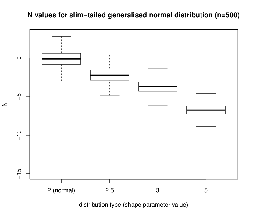
To illustrate this we compute the values of for bigger sample size, , for three different fat-tail distributions and three different slim-tail distributions. For fat-tail comparison we picked logistic, Student’s t with five degrees of freedom, and Laplace distributions, while for slim-tail comparison we considered generalised normal distribution with shape parameter ; the (standardised) generalised normal density for is given by
| (3.2) |
we refer to Nadarajah 2005 or Tumlinson et al. 2016 for more details. The results presented in Figure 3 confirm that the behaviour of is as expected.
Based on statistic values, one can construct a one-sided or two-sided statistical test with normality () as a null hypothesis. For brevity, we refer to such test as N normality test or simply N test.

4. Power of the test
In this section we check the power of the proposed test in a controlled environment. We focus on symmetric distributional alternatives (used e.g. in finance) when one wants to abandon the normality assumption due to fat-tail or slim-tail phenomena. Namely, we consider the Cauchy distribution, the Logistic distribution, the Laplace distribution, the Student’s t distribution with degrees of freedom parameter, and the generalised normal distribution (GN) with the shape parameter . Note that GN with and correspond to Laplace and normal distribution, respectively; see (3.2) for the GN density definition. In all cases, the location parameter is set to and the scale parameter is set to .
For completeness, we compare test results with well-established benchmark normality tests: Jarque–Bera test, Anderson–Darling test, and Shapiro–Wilk test. It should be noted that in contrast to these frameworks, statistic allows one to consider a specific heavy-tail (or slim-tail) alternative, i.e. positive (or negative) values of point out to heavy-tail (or slim-tail) alternative hypothesis. Consequently, we decided to construct right-sided (or left-sided) critical region for the fat-tailed (or slim-tailed) distributions. Nevertheless, for completeness, we include the results for two-sided critical regions in all cases.
For all alternative distribution choices we consider four different sample sizes, i.e. . For each , we simulate 2 000 000 strong Monte Carlo sample, and check for what proportion of simulations the tests reject normality at significance level .
All computations are performed in R 3.5.2. For benchmark normality testing we use multiple add-on R packages including gnorm (for GN simulation), stats (for Shapiro–Wilk test), nortest (Anderson–Darling test), and tseries (Jarque–Bera test). For better comparability, we used test-wise simulated rejection thresholds instead of theoretical -values returned by R functions; for computations, we used big strong Monte Carlo sample of size 10 000 000. In particular, note that while Jarque–Bera test has asymptotic distribution (with 2 degrees of freedom) under normality, this approximation may be inaccurate for small samples, and lead to non-meaningful (non-adjusted) p-values.
It should be noted that our framework specification is consistent with the one presented in Desgagné and Lafaye de Micheaux 2018, where a comprehensive normality tests comparison is made. In particular, results presented in Appendix C therein are perfectly consistent with results presented here (for all benchmark tests).22 2 Please note that results presented for Asymmetric Power Distribution (APD) with symmetry parameter correspond to results presented for Generalised Normal (GN) distribution; we refer to Section 2 in Desgagné and Lafaye de Micheaux 2018 for details.
For transparency, we have decided to consider fat-tail and slim-tail case separately. The results for fat-tailed distributions are presented in Table 1. The best performance of the right-sided test could be observed for almost all considered distributions. The fatter the tails the bigger the absolute difference between test power and JB test power, which could be considered as a second best choice. To check whether test statistic brings some novel results, we decided to check the proportion of simulations on which the normality assumption was rejected uiquely by among all considered tests; for comparison purposes, we checked the same for all other tests. The results for three selected distributions are presented in Table 2. It can be observed, that the unique rejection proportion for test is the highest among all tests and point out to the fact that statistic is taking into account sample properties that are not exploited by other tests.33 3 The results for other distributions are consistent with those presented in Table 2 and could be obtained from authors upon request. Finally, it should be noted that the performance of two-sided test is also quite good: the test outperforms both AD and SW in most of the considered cases.
The results for slim-tailed distributions are presented in Table 3. Both left-sided and two-sided test based on statistic substantially outperform all other tests on all datasets. This suggest that the proposed framework is also suitable when assessing slim-tailed distributions.
| Distr | n | JB | AD | SW | N (two-sided) | N (right-sided) |
| Cauchy | 20 | 86.2% | 88.0% | 86.6% | 85.5% | 89.0% |
| 50 | 99.5% | 99.7% | 99.6% | 99.7% | 99.8% | |
| 100 | 100.0% | 100.0% | 100.0% | 100.0% | 100.0% | |
| 250 | 100.0% | 100.0% | 100.0% | 100.0% | 100.0% | |
| Logistic | 20 | 14.9% | 10.6% | 11.7% | 11.1% | 15.6% |
| 50 | 25.9% | 15.9% | 19.6% | 21.2% | 28.9% | |
| 100 | 39.4% | 23.9% | 30.5% | 35.8% | 45.6% | |
| 250 | 66.7% | 46.7% | 57.0% | 67.8% | 76.4% | |
| Student’s t (2) | 20 | 56.7% | 52.9% | 52.9% | 52.9% | 60.1% |
| 50 | 88.2% | 85.8% | 86.3% | 89.2% | 92.3% | |
| 100 | 98.8% | 98.4% | 98.6% | 99.2% | 99.6% | |
| 250 | 100.0% | 100.0% | 100.0% | 100.0 | 100.0% | |
| Student’s t (5) | 20 | 22.9% | 17.1% | 18.6% | 18.1% | 23.9% |
| 50 | 43.0% | 30.2% | 35.5% | 38.4% | 46.8% | |
| 100 | 64.6% | 48.1% | 56.4% | 62.5% | 70.5% | |
| 250 | 92.0% | 81.8% | 88.2% | 92.8% | 95.4% | |
| Student’s t (10) | 20 | 12.3% | 8.8% | 9.8% | 9.2% | 12.5% |
| 50 | 20.6% | 12.0% | 15.5% | 15.7% | 21.6% | |
| 100 | 30.7% | 16.2% | 23.0% | 24.9% | 33.1% | |
| 250 | 52.3% | 28.5% | 41.7% | 47.8% | 57.9% | |
| Student’s t (20) | 20 | 8.1% | 6.4% | 6.8% | 6.5% | 8.2% |
| 50 | 11.4% | 7.2% | 8.7% | 8.4% | 11.5% | |
| 100 | 15.1% | 8.0% | 11.0% | 10.7% | 15.5% | |
| 250 | 22.9% | 10.3% | 16.2% | 17.2% | 24.8% | |
| Student’s t (30) | 20 | 6.9% | 5.8% | 6.1% | 5.9% | 7.0% |
| 50 | 8.9% | 6.2% | 7.1% | 6.8% | 8.9% | |
| 100 | 10.9% | 6.5% | 8.3% | 7.9% | 11.1% | |
| 250 | 15.0% | 7.4% | 10.7% | 10.7% | 16.0% | |
| Laplace/GN (1) | 20 | 30.2% | 27.2% | 26.1% | 26.4% | 35.4% |
| 50 | 55.6% | 54.5% | 52.1% | 59.3% | 69.1% | |
| 100 | 79.9% | 82.7% | 79.7% | 87.3% | 92.0% | |
| 250 | 98.7% | 99.6% | 99.2% | 99.8% | 99.9% | |
| GN (1.5) | 20 | 12.1% | 9.1% | 9.5% | 9.1% | 13.4% |
| 50 | 19.0% | 13.2% | 14.4% | 16.1% | 23.7% | |
| 100 | 27.9% | 19.8% | 21.5% | 27.3% | 37.5% | |
| 250 | 48.6% | 40.2% | 41.4% | 55.8% | 66.9% |
| Distr | n | JB | AD | SW | N (right-sided) |
|---|---|---|---|---|---|
| Logistic | 20 | 2.2% | 1.0% | 0.4% | 4.3% |
| 50 | 2.7% | 1.2% | 0.4% | 6.9% | |
| 100 | 2.7% | 1.0% | 0.3% | 9.3% | |
| 250 | 1.6% | 0.5% | 0.1% | 9.7% | |
| Student’s t (20) | 20 | 1.6% | 0.9% | 0.4% | 2.8% |
| 50 | 2.1% | 1.3% | 0.5% | 3.6% | |
| 100 | 2.5% | 1.4% | 0.5% | 4.7% | |
| 250 | 3.0% | 1.3% | 0.5% | 7.0% | |
| Laplace/GN (1) | 20 | 2.1% | 1.6% | 0.2% | 7.6% |
| 50 | 1.2% | 1.6% | 0.1% | 9.2% | |
| 100 | 0.3% | 0.7% | 0.0% | 5.1% | |
| 250 | 0.0% | 0.0% | 0.0% | 0.2% |
| Distr | n | JB | AD | SW | N (two-sided) | N (left-sided) |
|---|---|---|---|---|---|---|
| GN (2.5) | 20 | 2.4% | 4.5% | 4.1% | 5.4% | 8.6% |
| 50 | 1.3% | 5.5% | 4.6% | 8.0% | 13.6% | |
| 100 | 0.9% | 7.4% | 6.2% | 13.0% | 21.1% | |
| 250 | 4.3% | 14.5% | 12.9% | 29.1% | 41.3% | |
| GN (3) | 20 | 1.3% | 4.9% | 4.4% | 7.3% | 12.4% |
| 50 | 0.4% | 8.1% | 7.0% | 15.6% | 24.9% | |
| 100 | 0.8% | 15.0% | 13.7% | 31.2% | 44.1% | |
| 250 | 22.8% | 40.9% | 41.7% | 70.6% | 81.2% | |
| GN (5) | 20 | 0.5% | 8.2% | 7.8% | 15.9% | 25.4% |
| 50 | 0.1% | 23.0% | 24.3% | 47.2% | 61.2% | |
| 100 | 12.3% | 53.4% | 60.8% | 83.3% | 90.8% | |
| 250 | 97.0% | 96.7% | 99.1% | 99.9% | 100.0% | |
| GN (10) | 20 | 0.3% | 13.1% | 13.8% | 26.4% | 38.5% |
| 50 | 0.3% | 43.4% | 53.4% | 73.0% | 83.3% | |
| 100 | 50.0% | 84.9% | 94.6% | 97.7% | 99.1% | |
| 250 | 100.0% | 100.0% | 100.0% | 100.0% | 100.0% |
5. Mathematical framework and asymptotic results
In this section, we provide the explicit formulas for the conditional variance estimators, study their asymptotic behaviour, and show that is asymptotically normal.
First, we introduce the basic notation and provide more explicit formulas for sets , , and that were given in Section 2; see (2.1).
We assume that for mean parameter and standard deviation parameter . We use to denote the distribution of , to denote the standard normal distribution, and to denote the standard normal density. Following the usual convention, for any , we use to denote the random sample from and for , we use to denote the sample th order statistic.
For fixed partition parameters , where , we define the conditioning set
For brevity and with slight abuse of notation, we often write instead of . Then, the explicit formulas for sets , , and given in (2.1) are
| (5.1) |
where and is the unique negative solution of the equation
| (5.2) |
The approximate value of is ; we refer to (Jaworski and Pitera 2016, Lemma 3.3) for details. Note that (5.2) could be seen as a specific form of differential equation , where ; this could be used to determine similar ratios for other distributions.
Next, we give the exact definition of the conditional sample variance. For a fixed set , where , the conditional variance estimator on the set is given by
| (5.3) |
where denotes the floor of and
| (5.4) |
is the conditional sample mean. In particular, we set Recall that the test statistic is given by
| (5.5) |
where the normalising constant in (5.5) is approximately equal to ; we refer to Appendix A for the closed form formula for . Now, we are ready to state the main result of this section, i.e. Theorem 5.1.
Theorem 5.1.
Before we present the proof of Theorem 5.1 let us introduce a series of Lemmas and additional notation; proof techniques are partially based on those introduced in Stigler 1973. To ease the notation, for a fixed set , where , we define
Additionally, we set
where is the indicator function of set . It is useful to note that and follow the binomial distributions and , respectively; note that for and the distributions are degenerate with and .
Finally, for any sequence we introduce the notation of the directed sum that is given by
In Lemma 5.2, we show the consistency of the conditional sample expectation. Note that the statement of Lemma 5.2 does not explicitly rely on normality assumption. In fact, the proof is true under very weak conditions imposed on (e.g. continuity of the distribution function of ); similar statement is true for other lemmas presented in this section. Also, it should be noted that Lemma 5.2 and Lemma 5.3 show consistency and asymptotic distribution of the standard non-parametric Expected Shortfall estimator; see e.g. McNeil et al. 2010 for details.
Lemma 5.2.
For any , it follows that
Proof.
Let . For any , we get
Now, we show that
| (5.6) |
Due to the consistency of the empirical quantiles, we get and , as . Thus, using inequality
to prove (5.6), it is sufficient to show that Noting that
where
| (5.7) |
and, by the Law of Large Numbers, we conclude the proof of (5.6). The proof of
| (5.8) |
is similar to the proof of (5.6) and is omitted for brevity.
Next, we focus on the asymptotic distribution of the conditional sample mean; note that Lemma 5.3 is a slight modification of the result of Stigler 1973 for trimmed means. For completeness, we present the full proof.
Lemma 5.3.
For any , it follows that
for some constant .
Proof.
For brevity, we assume that and The remaining degenerate cases could be treated in the similar manner. Let . Define
As in the proof of Lemma 5.2, observe that
| (5.10) |
Now, we show that
| (5.11) |
Due to the consistency of the empirical quantiles, we get
as . Thus, using inequality
it is sufficient to show that converges in distribution to some non-degenerate distribution. Note that
where
| (5.12) |
and, by the Central Limit Theorem applied to , we get
Thus, using the Slutsky’s Theorem (see e.g. (Ferguson 1996, Theorem 6’)), we get
which concludes the proof of (5.11). Similarly, one can show that
| (5.13) |
Combining (5.11) with (5.13), and noting that
| (5.14) |
we can rewrite (5.10) as
where . Next, we have
where for , we set
Finally, noting that for we get and combining the Central Limit Theorem applied to with the Slutsky’s Theorem we conclude the proof; note that are i.i.d. with zero mean and finite variance. ∎∎
Next, we show that for the conditional variance estimator one can substitute the sample mean with the true mean without impacting the asymptotics. For any , where , the conditional variance estimator with known mean is given by
Lemma 5.4.
For any , it follows that , .
Proof.
Now, we study the asymptotic behaviour of the conditional variance estimator; this is a key lemma that will be used in the proof of Theorem 5.1. Moreover, this result may be of independent interest since it allows one to construct the asymptotic confidence interval for the conditional variance.
Lemma 5.5.
For any it follows that
where
| (5.15) |
Proof.
Due to Lemma 5.4, it is enough to consider instead of . For
we get
| (5.16) |
By the arguments similar to the ones presented in the proof of Lemma 5.3, we get
and
Thus, recalling (5.14), we can rewrite (5) as
where . Next, for , we set
| (5.17) |
and by straightforward computations we get and . Consequently, noting that
| (5.18) |
and using the Central Limit Theorem combined with the Slutsky’s Theorem, we conclude the proof. ∎∎
Finally, we are ready to show the proof of Theorem 5.1.
of Theorem 5.1.
For conditioning sets , , and given in (5.1), we define the associated sequences of random variables , , using (5.17). For any , we set
where is defined via (5.2). By the multivariate Central Limit Theorem (cf. (Ferguson 1996, Theorem 5)), we get where
Now, let Using (2.2), it is easy to see that
| (5.19) |
Consequently, by the arguments similar to the ones presented in the proof of Lemma 5.5 (see (5.18)), we can rewrite (5.19) as where and
Next, observing that and using the multivariate Slutsky’s Theorem (cf. (Ferguson 1996, Theorem 6)), we get where
| (5.20) |
Let and Observing that , and again using the Slutsky’s Theorem, we get To conclude the proof of Theorem 5.1, we need to show that is independent of and .
To do so, let us first show that for any , where , and the corresponding random variable given in (5.17), we get
| (5.21) |
where and is some fixed measurable function. From (Johnson et al. 1994, Section 13.10.1), we know that
| (5.22) | ||||
| (5.23) |
Consequently, the standardised mean and variance depend only on and . Recalling (5.17), we get
| (5.24) |
Combining this with equalities
we conclude the proof of (5.21).
The results presented in this section could be directly applied to various other non-parametric quantile estimators and to the unbiased variance estimators.66 6 In particular, this refers to the estimator implemented via quantile function in R that was used in Figure 1. This is summarised in the next two remarks.
Remark 5.6.
The standard formula for the whole sample (unbiased) variance uses instead of in the denominator. In the conditional case, this would be reflected in the different formula for (5.3), where is replaced by . Note that the statement of Theorem 5.1 remains valid for the modified conditional variance estimator due to the combination of the Slutsky’s Theorem and the fact that .
Remark 5.7.
When defining the conditional sample variance (5.3), we used and as the limits of the summation in (5.3) and (5.4). This choice corresponds to the non-parametric -quantile estimator given by .
In the literature there exist many different formulas for non-parametric quantile estimators, most of which are bounded by the nearest order statistics; see Hyndman and Fan 1996 for details. It is relatively easy to show that all results presented in this section hold true if we replace and by suitably chosen sequences that correspond to different empirical quantile choices. For completeness, we provide a more detailed description of this statement.
Consider sequences and such that and are bounded, and define . The corresponding conditional sample mean and variance are given by
Then, we can replace and by and in Theorem 5.1 as well as in all lemmas presented in the section.
Instead of showing a full proof, we briefly comment how to show consistency of quantile estimators as well as comment on counterparts of (5.7) and (5.12). All proofs could be translated using a very similar logic.
First, noting that for some we get and , it is straightforward to check that and are consistent -quantile and -quantile estimators; see e.g. (Serfling 1980, Section 2.3). Second, to show the analogue of (5.7), it is enough to use the boundedness of and , and note that and . Third, to show (5.12), it is enough to use boundedness of and note that for some we get .
6. Empirical example: case study of market stock returns
In this section we apply the proposed framework to stock market returns performing a basic sanity-check verification. Before we do that, let us comment on the connection between the 20-60-20 Rule and financial time series.
Assuming that describes financial asset return rates we can split the population using 20/60/20 ratio and check the behaviour of returns within each subset. If non-normal perturbations are observed only for extreme events, the 20/60/20 break might identify the regime switch and provide a good spatial clustering; this could be linked to a popular financial stylised fact saying that average financial asset returns tend to be normal, but the extreme returns are not – see Cont 2001 and Sheikh and Qiao 2010 for details. It should be emphasized that according to authors’ best knowledge, the link between this property and data non-normality was not discussed in the literature before.
The easiest way to verify this hypothesis is to take stock return samples for different periods, make the quantile–quantile plots (with standard normal as a reference distribution) and check if the clustering is accurate. In Figure 4, we present exemplary results for two major US stocks, namely GOOGL and AAPL, and two major stock indices, namely S&P500 and DAX; we took time-series of length 250 for different time intervals ranging in the period from 10/2015 to 01/2018.77 7 Data is downloaded from Yahoo Finance via R tidyquant package.


From Figure 4 we see that this division is surprisingly accurate: a very good normal fit is observed in the set (middle 60% of observations), while the fit in the tail sets and (bottom and top of observations) is bad. By taking different sample sizes, different time-horizons, and different stocks we can confirm that this property is systematic, i.e. the results are almost always similar to the ones presented in Figure 4.
While the presence of fat-tails in asset return distributions is a well-known observation in the financial world, it is quite surprising to note that the non-normal behaviour could be seen for approximately 40% of data. Also, test statistic can be used to formally quantify this phenomenon and to measure tail heaviness: the bigger the conditional standard deviation in the tails (in reference to the central part), the fatter the tails.
In the following, we focus on assessing the performance of the test statistic on market data. We perform a simple empirical study and take returns of all stocks listed in S&P500 index on 16.06.2018 that have full historical data in the period from 01.2000 to 05.2018. This way we get full data (4610 daily adjusted close price returns) for 381 stocks. Next, for a given sample size we split the returns into disjoint sets of length , and for each subset we compare the value of with the corresponding empirical quantiles presented in Figure 2. More precisely, using we perform a right-sided statistical test and reject normality (null) hypothesis if the computed value is greater than the empirical value , for .
To assess test performance, we compare the results with other benchmark normality tests: Jarque–Bera test, Anderson–Darling test, and Shapiro–Wilk test. While the non-normality of returns is a well-known fact, and all testing frameworks should show good performance, we want to check if our framework leads to some new interesting results. We check the normality hypothesis and compute two supplementary metrics that are used for performance assessment:
- -
Statistic T gives the total rejection ratio of a given test. It corresponds to the proportion of data on which the normality assumption was rejected at a given significance level; it is the ratio of rejected data subsamples to all data subsamples.
- -
Statistic U gives the unique rejection ratio of a given test. It corresponds to the proportion of data on which normality assumption was rejected at a given significance level only by the considered test (among all four tests); it is the ratio of uniquely rejected data subsamples to all data subsamples.
The combined results for all values of and are presented in Table 4.
| Desc | nr runs | n | rejects | JB | AD | SW | N | |
|---|---|---|---|---|---|---|---|---|
| T | 35052 | 1.0% | 50 | 31.5% | 25.9% | 17.3% | 23.2% | 25.9% |
| U | 1.9% | 0.6% | 0.3% | 3.1% | ||||
| T | 35052 | 2.5% | 50 | 39.6% | 32.4% | 22.9% | 28.3% | 32.5% |
| U | 2.4% | 0.9% | 0.3% | 3.9% | ||||
| T | 35052 | 5.0% | 50 | 47.9% | 38.6% | 29.1% | 33.7% | 39.6% |
| U | 2.4% | 1.3% | 0.4% | 5.1% | ||||
| T | 17526 | 1.0% | 100 | 52.8% | 45.2% | 31.8% | 41.3% | 46.1% |
| U | 2.2% | 0.6% | 0.3% | 4.4% | ||||
| T | 17526 | 2.5% | 100 | 61.3% | 52.9% | 38.8% | 47.6% | 54.3% |
| U | 2.2% | 0.7% | 0.2% | 5.1% | ||||
| T | 17526 | 5.0% | 100 | 68.4% | 59.7% | 45.7% | 53.4% | 61.3% |
| U | 2.2% | 0.8% | 0.2% | 5.3% | ||||
| T | 6858 | 1.0% | 250 | 88.5% | 82.1% | 71.2% | 79.3% | 85.4% |
| U | 1.0% | 0.4% | 0.1% | 3.8% | ||||
| T | 6858 | 2.5% | 250 | 91.8% | 86.8% | 77.7% | 83.7% | 89.4% |
| U | 0.7% | 0.2% | 0.1% | 3.0% | ||||
| T | 6858 | 5.0% | 250 | 93.9% | 89.7% | 82.4% | 86.9% | 92.0% |
| U | 0.5% | 0.2% | 0.0% | 2.5% |
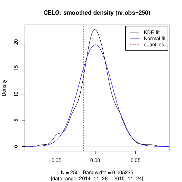
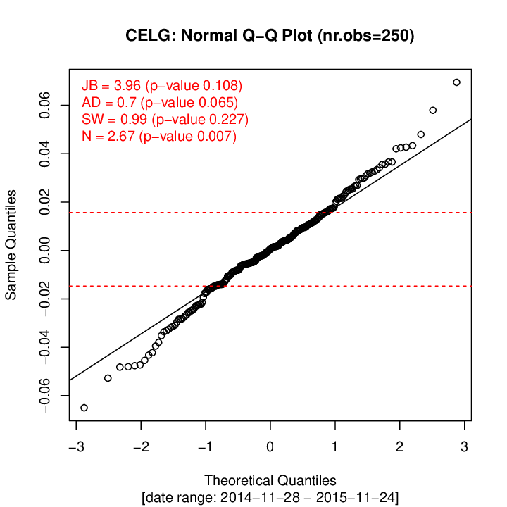
One can see that the statistic performs very well and gives the best results for all choices of . Surprisingly, our testing framework allows one to detect non-normal behaviour in cases when other tests fail: the outcomes of measure are material in all cases. For example, for and , the value of was equal to – this corresponds to almost of all rejected samples. The results are especially striking for , where the normality assumption was rejected in almost all cases (ca. 90%). While one might think that for such a big sample size the three classical tests should detect all abnormalities, our test still uniquely rejected normality in multiple cases. For , the normality was rejected for additional 262 samples ( of the population). For transparency, in Figure 5 we show exemplary data subset for which this happened.
7. Concluding remarks and other applications
In this paper we have shown that the test statistic introduced in (3.1) could be used to measure the heaviness of the tails in reference to the central part of distribution and could serve as an efficient goodness-of-fit normality test statistic. Test statistic is based on the conditional second moments, performs quite well on market financial data, and allows one to detect non-normal behaviour where other benchmark tests fail.
As mentioned in the introduction, most empirical studies suggest that the normality tests should be chosen carefully as their statistical power varies depending on the context. Our proposal proves to have the best test power in the cases when the true distribution is assumed to be symmetric and have tails that are fatter or slimmer than the normal one. It should be noted that our test is in fact based on the implicit distribution symmetry assumption. Indeed, in (3), the impact of left and right tail is taken with the same weight. Nevertheless, this could be easily generalised e.g. by considering only one of the tail variances; we comment on that later.
In Theorem 5.1 we proved that the asymptotic distribution of is normal under the normality null hypothesis. This allows us to study the shape of rejection intervals for sufficiently large samples. To obtain this result, in Lemma 5.5 we derived the asymptotic distribution of the conditional sample variance.
Also, we showed that the 20-60-20 Rule explains the financial stylised fact related to tail non-normal behaviour and provides surprisingly accurate clustering of asset return time series. Quite surprisingly, non-normality is visible for almost 40% of the observations.
In summary, we believe that tail-impact tests based on the conditional second moments are very promising and provide a nice alternative to the classical framework based e.g. on the third and fourth moments.
For example, the multivariate extension of the test statistic could be defined using the results presented in Jaworski and Pitera 2016, e.g. to assess the adequacy of using the correlation structure for dependence modeling. Also, this could be extended to any multivariate elliptic distribution using the results from Jaworski and Pitera 2017.
The construction of shows how to use conditional second moments for statistical purposes. In fact, one might introduce various other statistics that test underlying distributional assumptions. Let us present a couple of examples:
- -
We can test only the (left) low-tail impact on the central part by considering one of test statistics
- -
For any quantile-based conditioning sets and , and any elliptical distribution, one can introduce the statistic
where is a constant depending on the quantiles that define conditioning sets and the underlying distribution. Assuming that and (whole space), we get the proportion between the tail dispersion and overall dispersion. In this specific case, in the normal framework, we get
see (Jaworski and Pitera 2016, Section 3) for details.
Note that under the normality assumption all proposed statistics are pivotal quantities which facilitates an easy and efficient hypothesis testing; the asymptotic distribution for all statistics could be derived using similar reasoning as the one presented in Theorem 5.1.
Appendix A Closed-form formula for the normalising constant
In this section, we present the closed-form formula for the normalising constant from Theorem 5.1. For brevity, we omit detailed calculations and only present the outcome.
To ease the notation, for any , we set Then, for any , the standardised second, third, and fourth conditional central moments are given by
Moreover, the standardised conditional mean, conditional variance, and conditional kurtosis are equal to
Also, recall that , where is the unique negative solution of the equation
Now, we are ready to present the closed-form formula for ; see Corollary A.1.
Corollary A.1.
The normalising constant from Theorem 5.1 is given by
where for we have
and constants , , and are given by
Approximately, the value of is equal to .
Funding
Part of the work of the second author was supported by the National Science Centre, Poland, via project 2016/23/B/ST1/00479.
References
- (1)
- Alexander (2009) Alexander, C. (2009), Market Risk Analysis, Quantitative Methods In Finance, Vol. 1, John Wiley & Sons.
- Anderson and Darling (1954) Anderson, T. W. and Darling, D. A. (1954), ‘A test of goodness of fit’, Journal of the American Statistical Association 49(268), 765–769.
- Brockwell and Davis (2016) Brockwell, P. and Davis, R. (2016), Introduction to Time Series and Forecasting, Springer Texts in Statistics, Springer International Publishing.
- Cont (2001) Cont, R. (2001), ‘Empirical properties of asset returns: stylized facts and statistical issues’, Quantitative Finance 1(2), 223–236.
- Desgagné and Lafaye de Micheaux (2018) Desgagné, A. and Lafaye de Micheaux, P. (2018), ‘A powerful and interpretable alternative to the Jarque—Bera test of normality based on 2nd-power skewness and kurtosis, using the Rao’s score test on the APD family’, Journal of Applied Statistics 45(13), 2307–2327.
- Ferguson (1996) Ferguson, T. (1996), A Course in Large Sample Theory, Springer Science+Business Media Dordrecht.
- Hair et al. (2013) Hair, J., Black, W., Babin, B. and Anderson, R. (2013), Multivariate Data Analysis: Pearson New International Edition, Pearson Education Limited.
- Henze (2002) Henze, N. (2002), ‘Invariant tests for multivariate normality: a critical review’, Statistical Papers 43(4), 467–506.
- Hyndman and Fan (1996) Hyndman, R. J. and Fan, Y. (1996), ‘Sample quantiles in statistical packages’, The American Statistician 50(4), 361–365.
- Jarque and Bera (1980) Jarque, C. M. and Bera, A. K. (1980), ‘Efficient tests for normality, homoscedasticity and serial independence of regression residuals’, Economics Letters 6(3), 255 – 259.
- Jaworski and Pitera (2016) Jaworski, P. and Pitera, M. (2016), ‘The 20-60-20 rule’, Discrete & Continuous Dynamical Systems-Series B 21(4).
- Jaworski and Pitera (2017) Jaworski, P. and Pitera, M. (2017), ‘A note on conditional covariance matrices for elliptical distributions’, Statistics & Probability Letters 129, 230–235.
- Johnson et al. (1994) Johnson, N. L., Kotz, S. and Balakrishnan, N. (1994), Continuous univariate distributions, Vol. 1, Wiley & Sons, New York.
- Kaufman and Rousseeuw (2009) Kaufman, L. and Rousseeuw, P. J. (2009), Finding groups in data: an introduction to cluster analysis, Vol. 344, John Wiley & Sons.
- Madansky (2012) Madansky, A. (2012), Prescriptions for working statisticians, Springer Science & Business Media.
- McNeil et al. (2010) McNeil, A. J., Frey, R. and Embrechts, P. (2010), Quantitative risk management: concepts, techniques, and tools, Princeton University Press.
- Nadarajah (2005) Nadarajah, S. (2005), ‘A generalized normal distribution’, Journal of Applied Statistics 32(7), 685–694.
- Romão et al. (2010) Romão, X., Delgado, R. and Costa, A. (2010), ‘An empirical power comparison of univariate goodness-of-fit tests for normality’, Journal of Statistical Computation and Simulation 80(5), 545–591.
- Romesburg (2004) Romesburg, C. (2004), Cluster analysis for researchers, Lulu Press.
- Serfling (1980) Serfling, R. (1980), Approximation theorems of mathematical statistics, Wiley series in probability and mathematical statistics, Wiley & Sons, New York.
- Sheikh and Qiao (2010) Sheikh, A. and Qiao, H. (2010), ‘Non-normality of market returns: A framework for asset allocation decision making’, The Journal of Alternative Investments 12(3), 8–35.
- Stigler (1973) Stigler, S. M. (1973), ‘The asymptotic distribution of the trimmed mean’, Ann. Statist. 1(3), 472–477.
- Thadewald and Büning (2007) Thadewald, T. and Büning, H. (2007), ‘Jarque–Bera test and its competitors for testing normality – a power comparison’, Journal of Applied Statistics 34(1), 87–105.
- Thode (2002) Thode, H. C. (2002), Testing For Normality, Marcel Dekker.
- Tumlinson et al. (2016) Tumlinson, S., Keating, J. and Balakrishnan, N. (2016), ‘Linear estimation for the extended exponential power distribution’, Journal of Statistical Computation and Simulation 86(7), 1392–1403.
- Wilk and Shapiro (1965) Wilk, M. B. and Shapiro, S. S. (1965), ‘An analysis of variance test for normality (complete samples)’, Biometrika 52(3-4), 591–611.