Glide-symmetric magnetic topological crystalline insulators with inversion symmetry
Abstract
It is known that three-dimensional magnetic systems with glide symmetry can be characterized by a topological invariant together with the Chern number associated with the normal vector of the glide plane, and they are expressed in terms of integrals of the Berry curvature. In the present paper, we study the fate of this topological invariant when inversion symmetry is added while time-reversal symmetry is not enforced. There are two ways to add inversion symmetry, leading to space groups No. 13 and No. 14. In space group No. 13, we find that the glide- invariant is expressed solely from the irreducible representations at high-symmetry points in -space. It constitutes the symmetry-based indicator for this space group, together with another representing the Chern number modulo 2. In space group No. 14, we find that the symmetry-based indicator is given by a combination of the glide- invariant and the Chern number. Thus, in space group No. 14, from the irreducible representations at high-symmetry points we can only know possible combinations of the glide- invariant and the Chern number, but in order to know each value of these topological numbers, we should calculate integrals of the Berry curvature. Finally, we show that in both cases, the symmetry-based indicator for inversion symmetric systems leading to the higher-order topological insulators is directly related with the glide- invariant and the Chern number. As an independent approach to these results, we also construct all invariants from the layer construction for these space groups, and we show complete agreement with the above results for the topological invariants constructed from -space topology.
I Introduction
Over the decades, important roles of the relations between topology and symmetry in modern condensed matter physics have been recognized by the tour de force works. The trigger to encourage those researches is the discovery of a topological insulator (TI) Hasan and Kane 2010; Qi and Zhang 2011. TIs which appear in the presence of time-reversal symmetry (TRS) have attracted tremendous attention because of their unique and robust surface properties, and they are characterized by the topological invariant, where anti-unitariness of TRS plays a key role. Physicists have focused on the relations between topology and symmetry, and they have classified various topological phases ensured by combinations of internal symmetries, such as TRS, particle-hole symmetry, and chiral symmetry Schnyder et al. 2008; Kitaev 2009; Ryu et al. 2010.
Beyond internal symmetries, crystal symmetries of crystalline materials, such as spatial inversion, mirror, and rotational symmetries, play a crucial role to understand such topological phases. An introduction of crystal symmetries has enriched our knowledge for topological invariants Fu and Kane 2007; Teo et al. 2008. For instance, the topological invariant for the TI has a complicated expression when inversion symmetry is absent, while it is expressed as a simple formula as a product of parity eigenvalues at time-reversal invariant momenta (TRIMs) when inversion symmetry is preserved Fu and Kane 2007. In addition, since the seminal proposal of a topological crystalline insulator (TCI) Fu 2011, whose topological phase is ensured by crystal symmetries, various combinations of internal symmetry and crystal symmetries have turned out to give an immense list of new topological phases Mong et al. 2010; Hughes et al. 2011; Fang et al. 2012; Kargarian and Fiete 2013; Zhang et al. 2013; Ueno et al. 2013; Chiu et al. 2013; Morimoto and Furusaki 2013; Slager et al. 2013; Jadaun et al. 2013; Alexandradinata et al. 2014; Fulga et al. 2014; Benalcazar et al. 2014; Shiozaki and Sato 2014. In particular, the materials of the SnTe class are revealed to be mirror-symmetric TCIs, and they are the first material realization for the TCIs protected by crystal symmetries. Besides symmorphic symmetries, topological phases with nonsymmorphic symmetries have been vigorously discussed Parameswaran et al. 2013; Liu et al. 2014; Young and Kane 2015; Fang and Fu 2015; Shiozaki et al. 2015; Varjas et al. 2015; Watanabe et al. 2015; Po et al. 2016; Lu et al. 2016; Dong and Liu 2016; Chen et al. 2016; Kim and Murakami 2016; Shiozaki et al. 2016; Wieder and Kane 2016; Zhao and Schnyder 2016; Wang et al. 2016; Bzdušek et al. 2016; Yang et al. 2017; Takahashi et al. 2017; Furusaki 2017; Chen et al. 2018. Furthermore, a new class of TCIs hosting gapless boundary states whose dimension is less than for a -dimensional (D) insulating bulk has also been established, and they are dubbed a higher-order TI Benalcazar et al. 2017a; Benalcazar et al. 2017b; Langbehn et al. 2017; Song et al. 2017; Schindler et al. 2018a; Khalaf 2018; Schindler et al. 2018b; Song et al. 2018a; Khalaf et al. 2018.
For comprehensive classifications of topological phases protected by a space group (SG), an approach based on the -theory, which is a mathematical approach for gapped systems, has been adopted Freed and Moore 2013; Read 2017; Shiozaki et al. 2017; Shiozaki et al. 2018a; Shiozaki et al. 2018b. Other approaches, such as topological quantum chemistry and symmetry-based indicators, have been attracting research interest Kruthoff et al. 2017; Po et al. 2017; Bradlyn et al. 2017; Watanabe et al. 2018; in these approaches, topology of the bands and their compatibility relations are studied in the context of topological phases protected by SG symmetries. Particularly, symmetry-based indicators are useful in diagnosing topologically distinct band structures from the combinations of irreducible representations (irreps) at high-symmetry momenta Po et al. 2017; Watanabe et al. 2018. These approaches focus on different aspects of topological phases. In the -theory approach, one can comprehensively classify nontrivial phases, whereas an explicit formula for the topological invariant does not follow immediately from the theory. On the other hand, the symmetry-based indicator can reveal only the topological phases characterized by combinations of irreps. Thus, this theory cannot capture topological phases which cannot be known only from the irreps. Thus even with these powerful tools, one cannot reach a full understanding of nontrivial topological phases protected by SG symmetries, and there is much room for further investigation.
In this paper, we study topological phases when inversion symmetry is introduced in magnetic systems with glide symmetry, to see an intriguing interplay between topology and glide symmetry. We focus on topological phases in 3D spinless insulating systems protected by glide symmetry Fang and Fu 2015; Shiozaki et al. 2015, without any internal symmetry, such as TRS, particle-hole symmetry, and chiral symmetry. This symmetry class is known as class A, one of the 10 Altland-Zirnbauer symmetry classes Altland and Zirnbauer 1997. A glide operation is a product of a reflection and a fractional translational operation, and it is nonsymmorphic. Such topological phases are characterized by the topological invariant Fang and Fu 2015; Shiozaki et al. 2015 and the Chern number associated with the normal vector of the glide plane. The nature of a topology for the magnetic glide-symmetric systems is very different from that for the time-reversal symmetric TIs, ensured by the antiunitary property of the time-reversal operation, because of an absence of antiunitary symmetry in magnetic glide-symmetric systems. Since the glide symmetry is contained in many SGs, this glide-symmetric TCI phase, ensured by the topological invariant, can exist in many SGs as well. Nonetheless, the formula of the glide- invariant is quite complicated because it involves various terms of 2D integrals in momentum space Fang and Fu 2015; Shiozaki et al. 2015, and its behavior in the presence of additional symmetries has not been addressed. Therefore, it should be useful to make clear the fate of the glide- invariant in the presence of inversion symmetry in order to search for candidate materials of the glide-symmetric TCIs.
We consider the type-I magnetic SGs (MSGs), whose symbols are the same as those for the corresponding crystallographic SGs, because they do not contain time-reversal. For example, SG #7 in the text refers to the type-I magnetic SG G= (MSG7.24 in the notation of Bilbao Crystallographic Server Aroyo et al. 2006) which consists of the same unitary operations as that of SG #7. In this paper we study SGs #7, #13, and #14, which are the type-I MSGs 7.24, 13.65, and 14.75, respectively. If we add inversion symmetry to SG #7, it becomes either SG #13 or SG #14. In SG #13, thanks to inversion symmetry, we show that the topological invariant characterizing glide-symmetric systems can be written in terms of the irreps at high-symmetry points in the momentum space. In particular, we find that the glide-symmetric TCI is related to a higher-order TI ensured by inversion symmetry. This glide- invariant constitutes the symmetry-based indicator for this SG, together with another representing the Chern number modulo 2. In SG #14, we find that the symmetry-based indicator is given by a combination of the glide- invariant and the Chern number.
We also construct all invariants which characterize topology of layer constructions (LCs) for the systems with these SGs, in a similar way as in Ref. Song et al. 2018b. This construction is solely based on geometries of layers. We then show that these invariants completely agree with the set of topological invariants discussed so far in this paper. This means that they exhaust all the topological invariants in these SGs. To show this agreement, we find that it is convenient to modify the definition of glide- invariant, and this modification does not affect the results in the previous works on this topological invariant.
The organization in this paper is the following. In Sec. II, we briefly review general properties of glide-symmetric TCIs, together with the results of classifications based on the -theory and those from the symmetry-based indicators. Then we alter the definition of the glide- invariant from the previous works in Sec. III, in order to have complete agreement with the LC. We then derive new Fu-Kane-type simplified formulas of the topological invariant and establish representative models for the glide-symmetric TCI, for SG #13 in Sec. IV and for SG #14 in Sec. V, respectively. Throughout the paper, we restrict ourselves to bulk-insulating systems. In particular, we exclude gapless phases with topological band-crossing points in bulk, such as Weyl semimetals Murakami 2007; Wan et al. 2011.
II Preliminaries
In the present section, we will review basic properties of the glide-symmetric TCI Fang and Fu 2015; Shiozaki et al. 2015. We start by introducing the topological invariant characterizing the glide-symmetric system. We also introduce the previous works on topological phases for SGs #7, #13, and #14.
II.1 topological invariant for glide-symmetric magnetic systems
Here we briefly review the TCI ensured by glide symmetry proposed in Refs. Fang and Fu 2015; Shiozaki et al. 2015. To be concrete, let us begin with a 3D system invariant under a glide operation
| (1) |
where represents the mirror reflection with respect to the plane, and is a unit vector along the axis. Henceforth, the lengths of the primitive vectors are set to be unity. Then the Bloch Hamiltonian for the glide-symmetric system satisfies the equation
| (2) |
where is the -dependent glide operator representing . Since the Hamiltonian commutes with the glide operator on glide-invariant planes and , the Hamiltonian can be block-diagonalized into two blocks which are featured by the eigenvalues of . As we have , the eigenvalues of are given by
| (3) |
in spinless systems. Therefore, the two branches for those eigenvalues are related to each other, , and are interchanged when an eigenstate goes across the branch cut. This is a remarkable property of systems with nonsymmorphic symmetries with a fractional translation. Several previous works have addressed topological properties from the interplay between nonsymmorphic natures and other crystalline symmetries, such as 2D Dirac semimeatls Young and Kane 2015 and semimetallic structures in the layer groups Wieder and Kane 2016 in systems with TRS. Nonetheless, in this paper, we do not assume TRS.
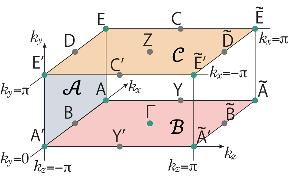
One can define the topological invariant for such glide-symmetric systems. Although the integral of Berry curvature for each glide sector on the glide-invariant planes can be defined, this quantity is not a quantized topological invariant due to the existence of the branch cut. Instead, a 3D gapped system with the glide symmetry is characterized by the topological invariant Fang and Fu 2015; Shiozaki et al. 2015 defined as
| (4) |
where , and are the integral regions shown in Fig. 1. We have defined the Berry connections
| (5) | ||||
| (6) |
and the corresponding Berry curvatures
| (7) | |||
| (8) |
where is the band index, the summation is over the occupied states, and is the Bloch wavefunction belonging to the glide sector with the glide eigenvalue . The Berry phase along a closed path is hence defined as
| (9) |
In Eq. (4), and are Berry phases with the paths taken as straight paths and , respectively, where the high-symmetry points are shown in Fig. 1. We take the gauge of the wavefunctions to be periodic along the direction. Namely, we take the wavefunction to be identical between and throughout the paper.
II.2 Previous works on topological phases for glide-symmetric systems with and without inversion symmetry in class A
Here we consider what happens to the glide- invariant, when inversion symmetry is added. SG #7 (), i.e., SG with the glide symmetry only, becomes either SG #13 () or SG #14 () by adding inversion symmetry. The difference between SG #13 and SG #14 comes from the position of inversion center; namely, while inversion center in SG #13 is within the glide plane, that in SG #14 is not. The resulting SGs have twofold () rotational symmetry in SG #13 and screw symmetry in SG #14.
For these three SGs, the -groups, the classifications of insulators including atomic ones, are known to be (SG #7), (SG #13) and (SG #14) Shiozaki et al. 2018a (Table 1). The symmetry-based indicators, which are defined as the quotients of the -groups by the abelian groups generated by atomic insulators, are trivial (SG #7), (SG #13) and (SG #14) Po et al. 2017; Watanabe et al. 2018 (Table 1). On the other hand, the topological invariants including the integral of Berry curvature on a 2D subspace of the Brillouin zone, which are classified by the terms in the Atiyah-Hirzebruch spectral sequence, are classified by (SG #7), (SG #13) and (SG #14) Shiozaki et al. 2018a (Table 1). However, physical meaning of each or factor in Table 1 is not obvious. The recent work in Ref. Ono and Watanabe 2018 gives physical interpretations of symmetry-based indicators in class A by analyzing those explicit formula in several key SGs. Nonetheless, from the symmetry-based indicators, one can neither study properties of topological invariants which cannot be expressed by symmetry-based indicators nor know how those topological invariants evolve when additional symmetry is added and the SG becomes its supergroup.
III Redefinition of the glide- invariant
In this section we revisit the definition of the glide- invariant . First we show how this topological invariant depends on the choice of the glide plane. We then introduce another topological invariant for glide-symmetric systems from the LC similarly to Ref. Song et al. 2018b. To achieve agreement between the two glide topological invariants, we show that it is better to change the definition of the glide- invariant from to (mod 2), where is the Chern number along the glide-invariant plane . Henceforth, refers the Chern number along the normal vector of the glide-invariant planes. We will also explain that this redefinition does not affect physical properties of the glide- invariant discussed in previous works Fang and Fu 2015; Shiozaki et al. 2015.
III.1 Gauge dependence of the glide- invariant
In systems with glide symmetry, we have two glide planes which are inequivalent under the lattice translation. For the glide operation given by Eq. (1), the glide planes are and . In such systems, when we take another glide operation given by
| (10) |
where is a mirror reflection with respect to the plane . Because where is a unit translation along the direction, this change of the glide operation switches the and sectors on the plane, while the glide sectors on the plane remain intact. Therefore, the value of the glide invariant changes from to
| (11) |
Its difference from the original value is given by
| (12) |
Because, the second term can be rewritten as , points , , and are specified in Fig. 1, we get
| (13) |
where is the Chern number along the - plane. Therefore, the value of the glide- invariant changes with the change of the glide plane, when is an odd integer.
III.2 Redefinition of the glide- invariant
In systems with glide symmetry, one can introduce a topological invariant associated with the glide symmetry, from the viewpoint of the real-space LC. This is a different approach from the approach from the -space topology, which led us to the glide- invariant . This approach of LC has been formulated in Ref. Song et al. 2018b for systems with TRS. We here extend this theory to systems with glide symmetry without TRS. We introduce a glide-invariant based on the LC by a straightforward calculation based on the geometry of the layers. The details of the definitions and calculations of are straightforward but lengthy, and are given in Appendix B.
By comparing this glide-invariant with the glide- invariant in Eq. (4), we find that they are not equal. Nonetheless, if we redefine the glide- invariant to be
| (14) |
it is equal to the glide invariant :
| (15) |
One may wonder whether this redefinition may invalidate the bulk-boundary correspondence of the glide- invariant , meaning the number of helical surface states in the gap given in the previous works Fang and Fu 2015; Shiozaki et al. 2015. Nevertheless, it is not the case, because in the arguments on the bulk-boundary correspondence in Refs. Fang and Fu 2015; Shiozaki et al. 2015, the Chern number is assumed to be equal to zero, in which case this redefinition does not alter the value of the glide- invariant: . Furthermore, the glide- invariant does not depend on the choice of the glide plane, as follows from Eq. (13). On the other hand, we remark that when , the glide- invariant may lose its meaning as the number of helical surface states, because its value is gauge dependent.
Thus the properties of the glide- invariant in Refs. Fang and Fu 2015; Shiozaki et al. 2015 remain valid even with this redefinition, and henceforth we will adopt the redefined glide- invariant (14). This redefinition is convenient when we compare the results with the LC, and is physically meaningful as we discuss later.
IV Glide-symmetric magnetic topological crystalline insulators for space group #13
In the present section, we consider SG #13, which is realized by adding inversion symmetry to SG #7. As explained in Sec. II.2, SG #13 has rotational symmetry, unlike SG #14. Here we derive a new formula of the glide- invariant (Eq. (16)) for SG #13. We then discuss how our new formula is related to symmetry-based indicators Po et al. 2017; Watanabe et al. 2018 and the topological invariants based on the -theory Shiozaki et al. 2018a. To check our results, we establish models realizing the topological phases in SG #13 based on the LC Song et al. 2018b.
IV.1 Topological invariants for SG #13
We will show that in SG #13, the topological invariant for the glide-symmetry system (mod 2) is given in terms of the irreps at high-symmetry points. For simplicity, here we consider the spinless case. Then, later we obtain
| (17) |
where is an eigenvalue of the rotation for the eigenstates in the sector at high-symmetry points , Y, Z, and C. In the following we show this formula by calculating from Eq. (16).
By adding an inversion around the origin to SG #7, we obtain SG #13. Then rotational symmetry around the axis ,
| (18) |
is also added to the symmetry operations. The key commutation relation between the glide operator and the rotational operator is given by
| (19) |
This will be used in the following discussion.
We now rewrite the formula of the glide- invariant (16) with the help of additional symmetries. First, the Berry curvature on the plane in Eq. (16) satisfies
| (20) |
owing to the symmetry. This immediately leads to
| (21) |
Next, we address the Berry curvature on the glide-invariant planes and . Equation (19) indicates that the glide sector for wavefunctions within the glide-invariant planes is unchanged under the rotation. Therefore, the Berry curvatures on those planes have to be an even function of and ,
| (22) |
where is either or .
Let us first consider the integral on the glide-invariant plane . From Eq. (22), we get
| (23) |
where is a half of the region given by , . Note that the does not change the glide sector of the eigenstates within the plane and we have taken the gauge to be periodic along the direction. Therefore, by using the Stokes’ theorem on the plane, we have
| (24) |
We have used the relation of the branch cut (mod ), points , , and are specified in Fig. 1.
Similarly, the terms on the other glide-invariant plane are given by
| (25) |
Consequently, from Eqs. (21), (24), and (25), we obtain a formula for the glide- invariant (16) as
| (26) |
where and are the eigenvalues () of the -th occupied state in the and sectors respectively, and and are the high-symmetry points on the plane shown in Fig. 1. To show this formula we used the properties of the sewing matrix as introduced in Ref. Fang et al. 2012 and its details are explained in Appendix A.
At the four high-symmetry points , Y, Z, and C, all the irreps are 1D, and their characters are shown in Table 2. Therefore, an alternative expression for is
| (27) |
where is the number of occupied states at the high-symmetry point with an irrep for the -group of SG #13.
Equations (26) and (27) explicitly depend on glide eigenvalues at high-symmetry points, which looks convention-dependent due to periodicity of the glide eigenvalues. Nevertheless, it can be rewritten in terms of the parity eigenvalues and thus is independent of conventions. By using compatibility relations for the irreps of SG #13, we can rewrite this formula for the glide- invariant as follows. We introduce the indicator for systems with inversion symmetry
| (28) |
where and are the number of occupied even-parity and odd-parity states at a TRIM , and the sum is taken over the eight TRIMs.
As mentioned earlier, we are assuming insulating systems, and in particular we exclude the Weyl semimetal phase, which means that this indicator is always an even integer Hughes et al. 2011; Ono and Watanabe 2018. Here we briefly explain why the indicator should be even. When the indicator is odd, which means that the parity of the Chern number on the plane and that on the plane are not equal, the gap should close somewhere between these planes, and the system is no longer an insulator Hughes et al. 2011. In such case, the gap closes at Weyl nodes, which are apices of the Dirac cones and carry topological charges characterized by the monopole density Murakami 2007; Wan et al. 2011. Therefore, the system is no longer an insulator, which is to be excluded here. Thus, the indicator is always an even integer and when it takes a value the system is a higher-order topological insulator with gapless hinge states. Then from the compatibility relations for SG #13, summarized in Appendix E, we obtain
| (29) |
Thus, in SG #13, the glide- invariant is equivalent to the indicator for inversion symmetry.
Since TRS is not assumed here, the Chern number on the - plane, which is parallel to the glide plane, can be nonzero. On the other hand, the Chern numbers on the - plane and on the - plane identically vanish due to the symmetry. As argued in Refs. Fang et al. 2012; Hughes et al. 2011, the Chern number on the - plane, which is perpendicular to the axis, is calculated in terms of eigenvalues up to modulo 2. On the plane, it is expressed as
| (30) |
where is the eigenvalue of the -th occupied state at the high-symmetry points, , Y, B, and A on the plane shown in Fig. 1. In the same manner, the Chern number on the plane is calculated from the product of eigenvalues at Z, C, D, and E, and, it is equal to calculated on the plane, since we have assumed a presence of the bulk gap. Otherwise, if the Chern numbers calculated at and at are not equal, the band gap vanishes somewhere between these planes Hughes et al. 2011, which occurs when is odd. On the other hand, this cannot occur if is even, i.e., .
IV.2 Symmetry-based indicators and -theory
Let us compare our results with the results on the symmetry-based indicator theory in the previous work Po et al. 2017; Watanabe et al. 2018. The symmetry-based indicator for SG #13 is Po et al. 2017; Watanabe et al. 2018. Following Ref. Po et al. 2017; Watanabe et al. 2018, we can show that one means the topological invariant for the glide-symmetric systems in Eq. (26), and that the other is the Chern number modulo 2 in Eq. (30). Thus, when inversion symmetry is present, and (mod 2) are both symmetry-based indicators, expressed in terms of irreps at high-symmetry points.
Let us discuss the relationship between the higher-order TI and these topological invariants. In a system with only inversion symmetry, obeying SG #2 (), symmetry-based indicators are given by Po et al. 2017; Watanabe et al. 2018, where the three factors of are weak indices for Chern insulators, while the factor of corresponds to a strong index in Eq. (28), counting the number of eigenstates below the Fermi energy having an odd parity. When or , it means that Weyl nodes appear in the momentum space. The case with corresponds to a higher-order TI, leading to an existence of 1D chiral hinge modes on the surface. In the present case of SG #13, Eq. (29) shows that the phase is equivalent to . Thus, the system with nontrivial glide- invariant is in the phase with , and it is a higher-order TI ensured by inversion symmetry. Thus they exhibit 1D chiral hinge modes.
On the other hand, in the classification based on the -theory Shiozaki et al. 2018a, the topological invariant given by the term expressing a topological invariant in terms of integrals of wavefunctions is the Chern number in SG #13 (Table 1). We conclude that the topological phase characterized by the glide- invariant is related to the higher-order TI with trivial weak indices , while that by an odd value of the Chern number is , where three ’s refer to the Chern numbers modulo 2 along the , and planes, and refers to the indicator in Eq. (28). This is among principle results of the present paper, and we check this scenario by constructing simple tight-binding models exhibiting topological phases in the following section.
IV.3 Layer constructions for glide- and inversion-symmetric systems
One can introduce various real-space topological invariants by the LC, similarly to Ref. Song et al. 2018b. In this LC for a SG, we introduce a set of planes, which are located periodically to be compatible with lattice translation symmetry. Here we consider each plane to be a 2D Chern insulator with a Chern number equal to . Then for a certain SG operation, such as inversion, rotation, and glide, we can show whether the configurations of the layers can be continuously trivialized or not, when the symmetry elements of SG other than symmetry for defining the invariant are ignored. Consequently, to indicate nontrivial configurations of planes we introduce an invariant for each SG operation.
To be more specific, we introduce a layer consisting of planes
| (31) |
where ’s are reciprocal vectors corresponding to the primitive vectors and . The integer is introduced because of the translation symmetry, and each layer consists of an infinite number of planes. Each layer is decorated with a 2D Chern insulator with a Chern number , with its orientation is given by a reciprocal lattice vector given by . Depending on SGs, we minimally introduce other layers to make the set of layers to be compatible with the given SG. Then we evaluate invariants for individual SG operations. The details are shown in Appendix B.
In SG #13, we can define four kinds of invariants, the Chern invariants , the glide invariant , the inversion invariant , and the invariant , only from geometric configuration of the layer as discussed in detail in Appendix B. The Chern invariant takes an integer value, while the other invariants and are defined modulo 2, and turns out to be always trivial. Then for every LC, one can evaluate these invariants, from which we establish relations between these invariants:
| (32) | ||||
| (33) |
as shown in Appendix B.
Now we can compare these invariants with the glide- invariant and the Chern number . One can calculate these two topological invariants for general layers and compare them with the invariants , , , and from the LC. Then we get
| (34) | ||||
| (35) |
Thus the construction of the topological invariants based on the LC completely agrees with the known topological invariants, the glide- invariant and the Chern number .
One can calculate the glide- invariant and the Chern number for general LCs, in order to show Eqs. (34) and (35) after a straightforward but lengthy calculation. From these results we can demonstrate generators of LCs for nontrivial values of topological invariants, i.e., minimal layer configurations for nontrivial combinations of the topological invariants. They are listed in Table 6 in Appendix B. In this section we study the two minimal LCs and in Table 6 for SG #13. These two LCs correspond to the glide-symmetric TCI and the Chern insulator phases in SG #13, respectively, and in this subsection we construct simple tight-binding models for them in order to examine our scenario. We show the outline of the calculations, and the details are presented in Appendix C.
IV.3.1 Glide-symmetric TCI phase:
We begin with the elementary LC (eLC) showing the glide-symmetric TCI phase (Fig. 2(a)). In the absence of inversion symmetry, i.e., for SG #7, a minimal configuration for a glide-symmetric TCI can be realized as a LC , representing 2D Chern insulators with along the plane placed at where is an integer. Then, the glide symmetry requires presence of other layers of a 2D Chern insulator with at , because the glide operation changes the sign of the Chern number along the plane. This model gives a nontrivial value of the topological invariant for glide-symmetric systems by a direct calculation.
We now consider the case when inversion symmetry is added, and SG becomes SG #13. Inversion symmetry fixes the value of to be , and the configuration allowed by symmetry is the one with the 2D Chern insulators on with and on with , where is the Chern number along the plane and is an integer (Fig. 2(a)). This is the LC with . Therefore, a representative Hamiltonian for the glide-symmetric TCI phase with additional inversion symmetry is obtained as
| (36) |
where and are Pauli matrices denoting the orbital and lattice degrees of freedom. We here set the Fermi energy to be . Hence, the corresponding -dependent glide operator and the -dependent inversion operator are
| (37) | ||||
| (38) |
Here, the subscript meant the matrix for the lattice degrees of freedom. The Hamiltonian (36) satisfies
| (39) | ||||
| (40) |
and these operators satisfy the commutation relation
| (41) |
which is just a Bloch form for given by the combination of Eqs. (18) and (19).
The Hamiltonian is gapped unless . The gap closes at when , at Y, Z when , and at C when . The glide- invariant is nontrivial (trivial) if ().
The effective Hamiltonian at the four high-symmetry points (, Y, Z, and C) in Eq. (26) can be written as
| (42) |
The irreps of the occupied states are summarized in Table 3. The sum of the numbers of the irreps at and Y and those of the irreps at Z and C in the occupied bands is odd at and the system is nontrivial, whereas it is even at and the system is trivial.
The parities at high-symmetry points at are shown in Fig. 2(c). Therefore, it is a higher-order TI with in SG #2 shown in Ref. Ono and Watanabe 2018. Thus, the glide-symmetric topological phase with the nontrivial invariant at is a higher-order TI in accordance with Sec. III.1.

| Y | Z | C | ||
|---|---|---|---|---|
IV.3.2 Chern insulator phase:
Next, we consider the eLC showing a weak 3D Chern insulator with a nontrivial Chern number along the - direction (Fig. 2(b)). In the absence of inversion symmetry, such a weak 3D Chern insulator phase can be realized as a stacking of 2D Chern insulators with parallel to the plane, located at with an integer . When we add inversion symmetry with inversion center at the origin, is set to be 0 or (Fig. 2(b)). To make to vanish, we choose . This layer is described as . Therefore, we have a representative Hamiltonian
| (43) |
Here, in order to make the model consistent with the glide symmetry, the primitive translation vector along the axis is taken as . Nonetheless, for the calculation of topological invariants from Eqs. (26) and (30) we should instead regard the primitive translation vector to be ; namely we double the unit cell along the direction. In this doubled unit cell, the Hamiltonian is rewritten as
| (44) |
The Hamiltonian indeed satisfies the relations in Eqs. (39) and (40) under the corresponding operators given by Eqs. (37) and (38).
This model shows phase transitions at . For example, we focus on the transition at . It is a trivial insulator at and a weak 3D Chern insulator with at , as can be seen from Eq. (43). Meanwhile, both and , the glide- invariant (26) is trivial. Therefore, the Hamiltonian realizes a topological phase with a nonzero Chern number but a trivial glide- invariant at as we intuitively expected. The parities at high-symmetry points in this model are shown in Fig. 2(d). It gives the values of the symmetry-based indicators as .
V Glide-symmetric magnetic topological crystalline insulators for space group #14
In this section, we consider SG #14 which is realized by adding screw symmetry to SG #7 having glide symmetry only. We mostly follow the argument for SG #13 in the previous section. Meanwhile, unlike SG #13, the inversion center in SG #14 is not within the glide plane, leading to the property that the glide sector on the plane changes by screw rotation. This makes the calculation very different from that in SG #13.
V.1 Topological invariants for SG #14
To begin with, we derive the glide- invariant in SG #14 by adding inversion symmetry to SG #7. Here we consider the spinless case for simplicity. In this case, we consider glide and inversion symmetries,
| (45) |
with its inversion center at the origin. It means that the glide plane is , and it does not contain inversion center, unlike that in SG #13. Then we get screw symmetry
| (46) |
The commutation relation between the glide and the screw operators is given by
| (47) |
Below, we mainly follow the same spirit of the previous section to derive a formula of the glide- invariant for SG #14. The symmetry-based indicator is for SG #14 Po et al. 2017; Watanabe et al. 2018. In the following, we show that the indicator gives information on the combination of the glide- invariant and the Chern number. Its formula here we find reads
| (48) |
where is an eigenvalue of the screw operation in the sector at the high-symmetry points , Y, D, and E. In the following we show this formula by calculating with given by Eq. (16). In the derivation, we should pay attention to the glide sectors and the branch cut.
Let us start with the term in Eq. (16) on the plane. The Berry curvature on the plane with should be an odd function of because of the screw symmetry. Therefore, we get
| (49) |
as similar to Eq. (21) in SG #13.
On the plane, because screw merely behaves as rotation, and it does not alter the glide sector, we have
| (50) |
which is the same as Eq. (24) in SG #13.
On the other hand, we confront a difference from the case of SG #13, when we evaluate the integral over the other glide-invariant plane . One cannot use the same trick as in SG #13 because screw changes the glide sectors, leading to the relation . Due to this relation, we find that the integral of the Berry curvature for the sector is a half of the integral of the total Berry curvature on the plane:
| (51) |
In the similar manner, noticing that
| (52) |
we can rewrite the terms on the plane as
| (53) |
As a consequence, by combining Eqs. (49), (50), and (53), we recast the formula for the glide- invariant into
| (54) |
where is the product of the screw eigenvalues over the occupied states for the sector at the high-symmetry point . An alternative expression is
| (55) |
Since the product of in Eq. (55) is equal to , the Chern number is found to be an even integer. Therefore, we have eventually shown that
| (56) |
This corresponds to the symmetry-based indicator for SG #14. Therefore, an alternative expression is
| (57) |
Furthermore, from the compatibility relations, one can also show that the indicator for inversion symmetry is directly related with this symmetry-based indicator Eq. (57):
| (58) |
Thus the value of the symmetry-based indicator for SG #14 gives possible combinations of the value of the glide- invariant and that of the Chern number . Meanwhile, one cannot uniquely determine the values of these topological numbers, solely from the symmetry-based indicator. Furthermore, both the glide- topological phase and a Chern insulator with the Chern number equal to (: integer) correspond to higher-order TIs with , ensured by inversion symmetry. It corresponds to phase. On the other hand, the term of the -theory classification Shiozaki et al. 2018a shows the topological invariant, i.e., the Chern number (Table 1). In the following section, we confirm these conclusions on the topological invariants by LCs.
V.2 Layer constructions for glide- and inversion-symmetric systems
One can define topological invariants based on the LC, as has been done for SG #13. In SG #14, we can define four kinds of invariants, the Chern invariants , the glide invariant , the inversion invariant , and the screw invariant , from geometric configurations of the layers with its details in Appendix B. The Chern invariant takes an integer value, while the other invariants , , and are defined modulo 2. Then for every LC, one can evaluate these invariants, from which we establish relations between these invariants:
| (59) | ||||
| (60) | ||||
| (61) |
We can compare these invariants with the glide- invariant and the Chern number , and we get
| (62) | ||||
| (63) | ||||
| (64) | ||||
| (65) |
Thus the topological invariants constructed from the LC completely agree with the known topological invariants, the glide- invariant and the Chern number .
One can calculate the glide- invariant and the Chern number for general LCs, in order to show Eqs. (62) to (65) after a straightforward but lengthy calculation. From these results we can demonstrate generators of LCs for nontrivial values of topological invariants, i.e., minimal layer configurations for nontrivial combinations of the topological invariants. They are listed in Table 6 in Appendix B. In this section we study the two minimal LCs and in Table 6 for SG #14. These two LCs correspond to the glide-symmetric TCI and the Chern insulator phases in SG #14, respectively, and in this subsection we construct simple tight-binding models for them in order to examine our scenario. We show the outline of the calculations, and the details are presented in Appendix D.
V.2.1 Glide-symmetric TCI phase:
First, a Hamiltonian exhibiting a glide-symmetric TCI is constructed by putting 2D Chern insulator layers with on the planes and those with on the planes, where is the Chern number along the plane and is an integer. Since this configuration becomes compatible with inversion symmetry by setting , the layer is now described as as shown in Fig. 3(a). Its representative Hamiltonian is given by
| (66) |
The form of the Hamiltonian is the same as Eq. (36), whereas the corresponding glide and inversion operators in momentum space are taken as
| (67) | ||||
| (68) |
Thus, we can see easily
| (69) |
which is Bloch form of .

As we mentioned in the previous section, the representative Hamiltonian in Eq. (66) closes the gap at when , at Y, Z when , and at C when . The irreps for the phases at and are summarized in Table 5. By calculating the screw eigenvalues at , D, Y, and E, the value of the symmetry-based indicator in our new formula of Eq. (56) is and is nontrivial. Since the Chern number should be 0 in this configuration, this nontrivial indicator is attributed to a nontrivial glide- invariant. Since this topological phase corresponds to in SG #2 by calculating the parities (Fig. 3(c)), this model is also a higher-order TI ensured by inversion symmetry.
V.2.2 Chern insulator phase:
Next we construct a model in the Chern insulator phase. To make a model compatible with inversion symmetry, we must put two 2D Chern insulator layers with within the lattice constant i.e., along the plane at and ( : integer) (Fig. 3(b)). It is written as . One can write down the model as
| (70) |
with the glide operator and inversion operator given by Eqs. (67) and (68), respectively. The Hamiltonian closes its gap at , and phase transitions occur. We here focus on the transition at , when the gap closes at , and the irreps at the both sides of the gap closing are given in Table 5. Surprisingly, they are the same as the previous model with the Hamiltonain for the glide-symmetric TCI () despite of the difference in the models. Because the Chern number for is obviously equal to two by construction, the glide- invariant is zero in this model. Thus, the Chern insulator with the Chern number equal to (: integer) is also a higher-order TI ensured by inversion symmetry which has in SG #2 Ono and Watanabe 2018 (Fig. 3(d)).
The two models (66) and (70) give the same values for the symmetry-based indicator. This is natural from our result in (56). From Eq. (56), the symmetry-based indicator is given by a combination of the glide- invariant and the Chern number, and therefore, although the values of the glide- invariant and the Chern number are different between the two models, the symmetry-based indicators are the same.
| Y | D | E | ||
|---|---|---|---|---|
VI Conclusion
In this paper we study the fate of the glide-symmetric topological invariant when inversion symmetry is added while TRS is not enforced. There are two ways to add inversion symmetry, leading to SGs 13 and 14. In SG #13, we derive the formula for the glide-symmetric topological invariant, and found that it is expressed in terms of the irreps at high-symmetry points. The symmetry-based indicator is , and one is this glide-symmetric topological invariant, while the other is the Chern number modulo 2 along the normal vector of the glide plane. On the other hand, in SG #14, the symmetry-based indicator is , and we show that this is equal to the sum of the glide-symmetric topological invariant and a half of the Chern number. Here we note that in this SG #14 the Chern number is always an even integer. It is interesting that the symmetry-based indicator gives a combination of two different topological invariants, while it does not uniquely determine the values of the individual topological invariants. We also construct invariants for LCs in these SGs. The list of invariants for LC turns out to agree with the topological invariants discussed in the present paper. We found the list of eLCs for SGs #13 and #14, and construct tight-binding models for these eLCs. By direct calculations, we can show that they have nontrivial values either for the glide- topological invariant and for the Chern number, which confirms the above conclusions.
Furthermore, we show that both the glide-symmetric TCI in SG #13 is a higher-order TI. In SG #14, the glide-symmetric TCI with the Chern number equal to an integer multiple of four is a higher-order TI. In SG #14, the Chern insulator with the Chern number equal to (: integer) and the trivial glide- invariant is also a higher-order TI. Nevertheless, in the Chern insulators the surface is gapless, and one cannot call the latter case in SG #14 a higher-order TI in the strict sense because the gapless hinge states are always hidden behind the gapless surface states due to the nonzero Chern number.
Our results will be useful for gaining insights for relating various topological phases. So far, various topological phases have been discovered by means of powerful methods, while their mutual relationships are not obvious in general. For example, we have shown that the glide-symmetric TCI becomes the higher-order TI in the presence of inversion symmetry, but such an equivalence is far from obvious from the known formula (4). Because the glide symmetry is one of the fundamental symmetries in crystals, and it is contained in many SGs, the present study will provoke studies on relating various topological invariants in some SGs and those in their supergroups.
It must be an intriguing and promising topic to search real materials of the glide-symmetric spinless TCI and the higher-order TI. Since our work have mainly discussed spinless systems, it does not suffer from the constraint of strong spin-orbit coupling when one does first-principle calculations. Nonetheless, we have not found any candidate materials so far, since it requires breaking of TRS. For realizing systems breaking of TRS but preserving glide symmetry or inversion symmetry, one candidate is magnetic insulators, such as insulators in magnetic field or localized spin systems. Bosonic systems, such as magnonic systems or photonic crystal systems in magnetic field, are one of the best candidates to find specific materials realizing these physics Lu et al. 2016. From the results in this paper, it is also promising to discover new TCI materials or the higher-order TI materials.
Acknowledgements.
We appreciate Tiantian Zhang for fruitful discussions. This work was supported by Grant-in-Aid for Scientific Research No, 26287062 and No, 18H03678. H. K. is supported by Japan Society for the Promotion of Science (JSPS) KAKENHI Grant-in-Aid for JSPS Fellows Grant No. JP17J10672. K. S. is supported by PRESTO, JST (JPMJPR18L4).Appendix A Sewing matrices with twofold rotational or screw symmetry
We exploit several convenient quantities argued in Ref. Fang et al. 2012 for evaluating the integral of the Berry curvature in the presence of additional rotational symmetry or screw symmetry.
First, we define a sewing matrix . The Bloch Hamiltonian having a point group symmetry satisfies , where is an operator corresponding to the point-group operation , and is transformed from by . From the operator which acts on the Bloch wavefunction , we define a corresponding operator , which acts on the occupied cell-periodic eigenstates . Then, we define a unitary matrix as
| (71) |
where and run over the occupied states. At the wavevector invariant under , the Hamiltonian commutes with , so that we can find the common eigenstates of the operators and . Here, the sewing matrix should be diagonal at such a high-symmetry point ,
| (72) |
where is the eigenvalue of for the th band. Therefore, the determinant of is given by the product of the eigenvalues of occupied eigenstates at ,
| (73) |
This quantity is gauge invariant because the determinant does not depend on the choice of basis.
Apart from the Berry phase, we also define a path-ordered exponential of the Berry connection,
| (74) |
evaluated in the subspace of the occupied states, along the path from to not necessarily being a closed path.
We can relate some formulas containing the Berry phase in the main text to rotation or screw eigenvalues, following Ref. Fang et al. 2012. As an example, here we show the detail of Eq. (26). The path-ordered integral along Y Y can be rewritten in terms of the eigenvalues. Due to the symmetry,
where is the sewing matrix for the operator, restricted within the subspace at the high-symmetry point , and is the eigenvalue for the sector at the high-symmetry point .
Appendix B Layer construction
In this Appendix, we consider a LC in class A for SGs #7, #13, and #14. In Ref. Song et al. 2018b, a LC is introduced for time-reversal-invariant systems, and in this previous work, each layer is decorated with a 2D TI and a 2D mirror TCI. In contrast, in the present paper, because we do not assume TRS, we decorate each layer with a 2D Chern insulator. We then construct all invariants based on each space-group operations, based solely on geometric properties of the layers. Then we show that these set of invariants are in complete agreement with the topological invariants based on -space geometry discussed in the main text of the paper. Based on these arguments, we show eLCs, which constitute a basis for the values of topological invariants.
B.1 setup
A layer is a set of planes given by the Miller indices displaced from the origin by (). It is given by
| (75) |
where ’s are reciprocal vectors corresponding to the primitive vectors and the integer is introduced because of the translation symmetry.
We then formulate general LCs, in the similar way as in Ref. Song et al. 2018b. In a given SG , symmetry property of a layer is described by its little group, which is defined as a subgroup of that leaves invariant:
| (76) |
Then, must also be a SG containing the full translation subgroup since by definition any lattice vector would translate the layer. We can get a finite number of cosets of for SG ,
| (77) |
Thus, we have a set of symmetric layers
| (78) |
by applying all the coset representatives on . An eLC is obtained by decorating the layers in with a 2D Chern insulator with a Chern number .
B.2 topological invariants for glide-symmetric systems
First of all, we consider how a general layer gives topological invariants in SG #7. Then, we expand our argument to SG #13 and SG #14 by adding inversion symmetry. Then, inversion symmetry and either rotational symmetry or screw symmetry are added as generators. We briefly explain how topological invariants can be calculated or added by these symmetries. Here we construct topological invariants associated with respective symmetry operations. We focus on one of the symmetry operations in the given SG, and in constructing a topological invariant associated with the symmetry operation, we neglect all the other symmetry operations in SG. We then construct possible LCs compatible with SG, and see whether each LC can be trivialized by deforming it while keeping its invariance under the focused symmetry operation. For example, in considering a glide invariant , we construct LCs satisfying the glide operation only, and then deform the LCs while keeping the glide symmetry, to see whether the LCs can be trivialized. This consideration leads to the definition of the glide topological invariant .
B.2.1 Chern invariant
The Chern number along a reciprocal lattice plane normal to one of the primitive vectors is written as defined as
| (79) |
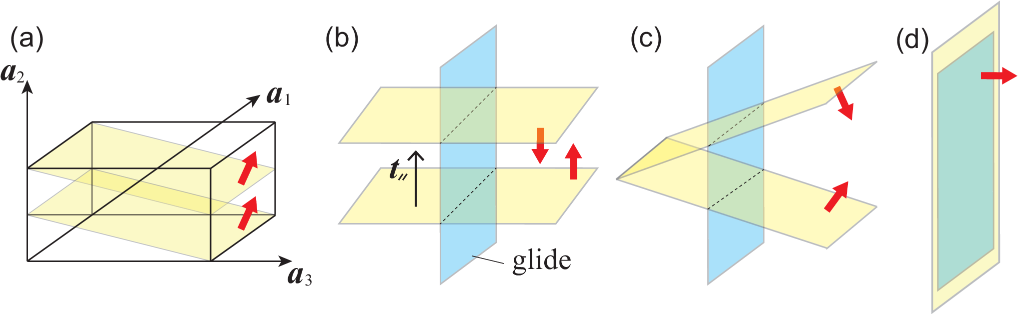
where is a unit vector along and the integral is taken over the 2D Brillouin zone on the plane . For a layer , it is equal to the number of intersections of with an axis parallel to the within the unit cell (Fig. 4 (a)). One can see easily its intersections with as
| (80) |
respectively. Thus, the Chern numbers associated with three primitive lattice vector should be given by
| (81) | ||||
| (82) | ||||
| (83) |
where is a general LC. Namely, it can be written as
| (84) |
where for the layer .
B.2.2 glide invariant
In addition, we can find a glide invariant for a glide-symmetric systems based on the LC in the similar way as in time-reversal-invariant systems treated in Ref. Song et al. 2018b. In glide-invariant systems, there are two glide planes in a unit cell, which are displaced by a half of the primitive translation vector. In constructing the glide invariant , we should first choose one of the glide planes, and we fix this choice throughout our theory.
In our case each layer is decorated with the 2D Chern insulator because TRS is not assumed, whereas in Ref. Song et al. 2018b, each layer is decorated with the 2D TIs. Nonetheless, nontrivial LC configurations are similar, classified into two types. In the first type of the nontrivial LC configuration, the glide plane is included in one of the layers in the LC (Fig. 4 (d)). It is characterized by the glide-occupation number (glide-ON) where specifies the glide plane. In the second type of the nontrivial LC configuration, there is a pair of layers which are connected by the glide operation (Fig. 4 (b)), which can be continuously deformed into the previous case (see Fig. 4 (c)). It is represented by a glide-stacking number (glide-SN) . Similarly to the cases in Ref. Song et al. 2018b, two pairs of such layers can be trivialized. Therefore, the resulting topological invariant is defined modulo 2, and one can write the glide invariant as
| (85) | ||||
| (88) |
We again emphasize that in Eq. (B.2.2), refers to the glide plane which we have chosen from the two different choices of the glide plane.
B.2.3 inversion invariant
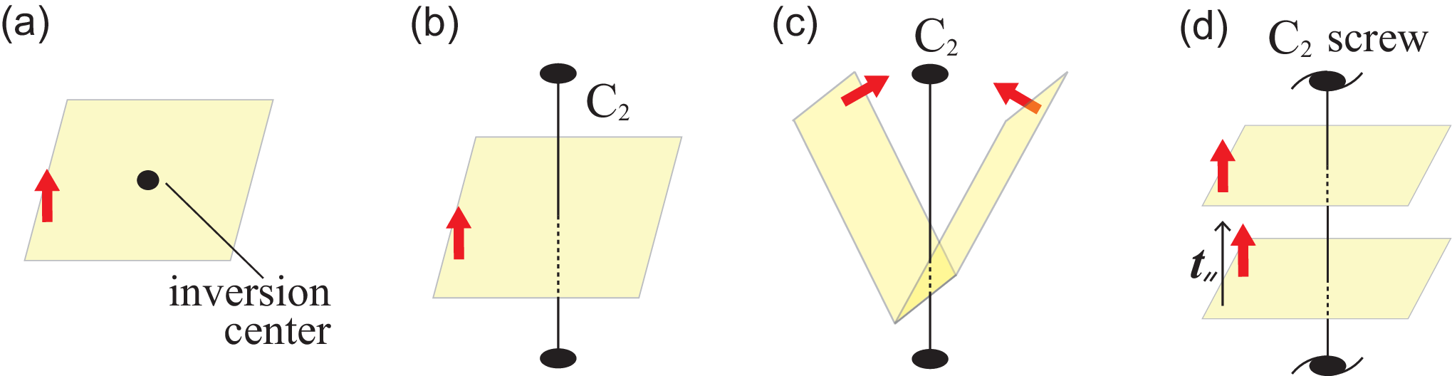
Systems with inversion symmetry have eight inversion centers within a unit cell. We first choose one of the inversion centers, and we fix the choice throughout our theory. If a layer in the LC includes the inversion center (Fig. 5 (a)), this LC cannot be trivialized as long as the inversion symmetry is preserved. Meanwhile, if the inversion center is occupied by two layers decorated with the 2D Chern insulator, one can trivialize this configuration up to the creation of the atomic insulator at the center of inversion. Thus the inversion invariant can be written as a inversion-ON of modulo 2:
| (89) | ||||
B.2.4 rotation invariant
In a similar manner, the rotation invariant is obtained. A layer of the 2D Chern insulator is invariant only when the plane is perpendicular to the axis (Fig. 5 (b)), and this layer can be trivialized, as we see from Fig. 5 (c). Consequently, the rotation invariant is always trivial:
| (92) |
It is a remarkable result, because the rotation invariant is always trivial in the system without TRS, while it is not in the presence of TRS Song et al. 2018b. In the presence of TRS, 2D TI layers are used for LCs, and the rotation invariant becomes nontrivial when a TI layer includes the axis. On the other hand, in our case where TRS is not enforced, layers of a 2D Chern insulator are used. In this case, the configuration where a layer of a 2D Chern insulator includes the axis is not invariant, unlike the case with TRS. Thus, there is no topologically nontrivial configuration for the rotation invariant.
B.2.5 screw invariant
In systems with screw symmetry the topological invariant is defined by a screw-SN. The nontrivial LC configuration is the LC with a pair of layers combined by the screw operation. In such cases, one pair of layers combined by screw symmetry cannot be trivialized (Fig. 5(d)), while two pairs can be trivialized. Thus we get
| (93) | ||||
| (94) |
where is a screw vector, and is equal to a half of a lattice translation vector.
B.3 Convention dependence of topological invariants
As remarked in Ref. Song et al. 2018b, topological invariants in the previous section depend on the conventions. For example, there are eight inversion centers in a unit cell in the presence of inversion symmetry, and we should choose one inversion center among them in defining an inversion invariant . When we choose the inversion center at the origin, passing the origin has whereas has because it does not pass the inversion center. On the other hand, when we choose the inversion center at , has whereas has . Thus, the inversion invariant depends on the convention on the choice of the inversion center among the eight inversion centers in the unit cell. Meanwhile, when we consider an LC with two eLC passing all eight inversion centers in a unit cell, the inversion invariant is independent of the choice of the inversion center, and the system is considered to be topologically nontrivial. Similarly, the glide-ON is also dependent on the convention. There are two glide planes within the unit cell, displaced from each other by half the primitive translation vector, and the glide invariant depends on the choice. When the LC occupies both of these glide planes odd times each, the glide invariant is nontrivial, irrespective of the choice of the glide plane, as is similar to the cases with time-reversal symmetry in Ref. Song et al. 2018b
In our cases in SG #13 as an example, the configuration in Fig. 2(a) has a nontrivial inversion invariant , irrespective of the convention of the inversion center since the layers pass all the eight inversion centers in the unit cell. Meanwhile, in the configuration in Fig. 2(b), the inversion invariant depends on the convention. In SG #14, both of the two configurations in Figs. 3(a)(b) have a convention-independent nontrivial inversion invariant ,
B.4 Invariants for layer constructions
Based on the definitions of the invariants given above, one can calculate their values for LCs in SGs #7, #13 and #14. We note that in the glide symmetry and in the inversion symmetry, we choose the glide planes and inversion centers to be the standard ones given in the main text, which are the same as those in the Bilbao Crystallographic Server Aroyo et al. 2006.
B.4.1 SG #7
In SG #7, only the Chern invariants and the glide invariant are defined. In the calculation we note that the glide operator transforms the layer to
| (95) |
Note that it is not written as . Therefore, the Chern numbers for the LC in SG #7 are given as
| (96) | ||||
| (97) | ||||
| (98) | ||||
| (99) |
where the classification is necessary for distinguishing the cases and . Here and follows from glide symmetry.
The glide invariant is given by
modulo 2. We note that the glide plane is chosen to be , and not . That is why (B.4.1) does not contain in the first case of .
B.4.2 SG #13
SG #13 is constructed from SG #7 by adding the inversion symmetry. The inversion transforms the layer into . This additional inversion symmetry doubles the number of layers, if the additional layers are not identical with the original ones, For the layer , the values of the Chern invariants are obtained as follows:
| (102) | ||||
| (103) | ||||
The glide invariant and the inversion invariant are calculated, and they turn out to be exactly equal;
modulo 2.
B.4.3 SG #14
SG #14 is constructed from SG #7 by adding inversion symmetry. For the layer , the values of the Chern invariants are obtained as follows:
| (111) | ||||
| (112) | ||||
The glide invariant is given by
modulo 2.
The inversion invariant is given by
modulo 2.
The screw invariant is given by
modulo 2.
They are related by the following equations:
| (127) | ||||
| (128) |
B.5 Elementary layer constructions
Following the argument in Ref. Song et al. 2018b, we can find eLCs in SGs #7, #13, and #14 summarized in Table 6. All SGs listed here have two independent topological invariants as we have seen in this paper, Therefore, each SG has two eLCs.
Appendix C Layer construction for SG #13
In this section we show the detailed construction of the models for the glide-symmetric TCI phase and the Chern insulator phase in SG #13. The symmetry generators are given by
| (129) |
C.1 Glide-symmetric TCI phase in the layer construction ()
We first calculate the topological invariants for the LC . The model Hamiltonian is given by putting a Chern insulator with on the plane at with inversion symmetry, which is written as
and making copies by the glide transformation
The Hamiltonian reads
Let us introduce the -space basis
| (130) |
The glide and inversion operations are represented as
Thus, the -space Hamiltonian and symmetry operators are given by
The rotation is given by
Let us compute the indicator for . At the high-symmetry points, the Hamiltonians and the symmetry operators within the occupied states are shown in the following table. Here an overall positive coefficients are omitted for simplicity.
Therefore, the glide- invariant becomes
i.e., . As a result, is equal to 1 for , and for other values of .
C.2 Chern insulator phase in the layer construction ()
We here calculate the topological invariants for the LC . The model Hamiltonian is given by putting a Chern insulator with on the plane at with inversion symmetry, which is written as
As noted in Sec. IV C, we first take the length of the unit cell along the direction to be , in order to make the model compatible with the glide symmetry. We then make copies by the the translation ,
and the glide operation is given by
In the momentum space, the Hamiltonian and symmetry operators are represented
This is a two-band model, when the primitive vector along the axis to be . One can formally regard the primitive vector along the axis to be , which renders this model to a four-band model. Let us introduce the -space basis
| (131) |
Then the Hamiltonian is given by
The rotation is
Let us compute the indicator for . At the high-symmetry points, the Hamiltonians and the symmetry operators within the occupied states are
Therefore, the glide- invariant is calculated as
for all the values of and it turned out to be trivial. On the other hand, this model has for and for by construction.
Appendix D Layer construction for SG #14
In this section we show the detailed construction of the models for the glide-symmetric TCI phase and the Chern insulator phase in SG #14. The symmetry generators are given by
| (132) |
D.1 Glide-symmetric TCI phase in the layer construction ()
We first calculate the topological invariants for the LC . The model Hamiltonian is given by putting a Chern insulator with on the plane at with inversion symmetry, which is written as
and making copies by the glide transformation
The Hamiltonian reads
Let us introduce the -space basis
| (133) |
The glide and inversion operations are represented as
Thus, the -space Hamiltonian and the symmetry operators are given by
The screw operation is
Let us compute the indicator for . At the high-symmetry points, the Hamiltonians and the symmetry operators within the occupied states are
Therefore, the symmetry-based indicator becomes
One can calculate the value of for other values of . As a result, is equal to for and zero otherwise. By construction, we know for this model, and therefore we get for and otherwise.
D.2 Chern insulator phase in the layer construction ()
We here calculate the topological invariants for the LC . The model Hamiltonian is given by putting a 2D Chern insulator with on the plane at with inversion symmetry, which is written as
and making copies by the glide transformation and the translation ,
In the momentum space, the Hamiltonian and symmetry operators are represented by
Let us compute the indicator for . The screw operation is
At the high-symmetry points, the Hamiltonians and the symmetry operators within the occupied states are
Note that the Hamiltonians at the high-symmetry points are the same as the case of . Therefore, the symmetry-based indicator is identical with the previous one:
i.e. for , and otherwise. By construction, we in fact have for , and otherwise.
Appendix E Irreducible representations
In this section, we summarize the lists of irreps and compatibility relations for SGs #13 and #14. They are shown in Tables 7 for SG #13 and 8 for SG #14. We used the database, the Bilbao Crystallographic Server Aroyo et al. 2006. We show the numbers of irreps at high-symmetry points in the rightmost column of each table, so as to satisfy the compatibility relations. Namely, within the Abelian group generated by the irreps at high-symmetry points, the integer parameters in these numbers corresponds to the generators of its subgroup satisfying the compatibility relations. Therefore, the number of the parameters is equal to the dimension in in Ref. Po et al. 2017, and we have for SG #13 and for SG #14. From these numbers, one can show various relations for the numbers of irreps. As an example, here we show Eqs. (29) for SG #13 and (58) for SG #14.
In SG #13, from the Table 7, the glide- invariant is equal to . Similarly, the Chern number modulo 2 is given by . On the other hand, the index is calculated by counting the number of odd-parity states at all the TRIMs, and we get . Therefore, we verify that is one half of the index , from the compatibility relation for irreps.
In SG #14, the combinations of the value of the glide- invariant and that of the half of the Chern number is given by the number of the irreps at , Y, D, and E. It can be calculated as . On the other hand, the index for inversion symmetric systems is equal to . Therefore, we conclude that both the glide- topological phase and a Chern insulator with the Chern number equal to (: integer) correspond to the topological phase with .
Appendix F Spinful systems
In this section, we will consider the spinful systems of SG #13 and SG #14. The formulas for SG #13 in Eq. (26) and SG #14 in Eq. (56) can be also applied in the same manner to the spinful systems, because the commutation relations between the glide and rotation/screw operations in Eqs. (19) and (47) are unchanged.
From the database Aroyo et al. 2006, we summarize the lists of irreps for spinful SGs #13 and #14 in Tables 9 and 10. The double-valued representation of is given by times to . For simplicity, we have omitted some information; matrix representations are same in Tables 7 and 8 except for
| (134) |
for and numbers of irreps are twice those in Tables 7 and 8, respectively.
The formulas for spinful systems of SG #13 and SG #14 are given by
| (135) | ||||
| (136) |
where and are an eigenvalue of the rotation/screw for the eigenstates in the sector,
| (137) |
at high-symmetry points , Y, Z, and C in SG #13 and , Y, D, and E in SG #14, respectively.
References
- Hasan and Kane (2010) M. Z. Hasan and C. L. Kane, Rev. Mod. Phys. 82, 3045 (2010).
- Qi and Zhang (2011) X.-L. Qi and S.-C. Zhang, Rev. Mod. Phys. 83, 1057 (2011).
- Schnyder et al. (2008) A. P. Schnyder, S. Ryu, A. Furusaki, and A. W. W. Ludwig, Phys. Rev. B 78, 195125 (2008).
- Kitaev (2009) A. Kitaev, in AIP Conference Proceedings, Vol. 1134 (AIP, 2009) pp. 22–30.
- Ryu et al. (2010) S. Ryu, A. P. Schnyder, A. Furusaki, and A. W. Ludwig, New Journal of Physics 12, 065010 (2010).
- Fu and Kane (2007) L. Fu and C. L. Kane, Phys. Rev. B 76, 045302 (2007).
- Teo et al. (2008) J. C. Y. Teo, L. Fu, and C. L. Kane, Phys. Rev. B 78, 045426 (2008).
- Fu (2011) L. Fu, Phys. Rev. Lett. 106, 106802 (2011).
- Mong et al. (2010) R. S. K. Mong, A. M. Essin, and J. E. Moore, Phys. Rev. B 81, 245209 (2010).
- Hughes et al. (2011) T. L. Hughes, E. Prodan, and B. A. Bernevig, Phys. Rev. B 83, 245132 (2011).
- Fang et al. (2012) C. Fang, M. J. Gilbert, and B. A. Bernevig, Phys. Rev. B 86, 115112 (2012).
- Kargarian and Fiete (2013) M. Kargarian and G. A. Fiete, Phys. Rev. Lett. 110, 156403 (2013).
- Zhang et al. (2013) F. Zhang, C. L. Kane, and E. J. Mele, Phys. Rev. Lett. 111, 056403 (2013).
- Ueno et al. (2013) Y. Ueno, A. Yamakage, Y. Tanaka, and M. Sato, Phys. Rev. Lett. 111, 087002 (2013).
- Chiu et al. (2013) C.-K. Chiu, H. Yao, and S. Ryu, Phys. Rev. B 88, 075142 (2013).
- Morimoto and Furusaki (2013) T. Morimoto and A. Furusaki, Phys. Rev. B 88, 125129 (2013).
- Slager et al. (2013) R.-J. Slager, A. Mesaros, V. Juricic, and J. Zaanen, Nat. Phys. 9, 98 (2013).
- Jadaun et al. (2013) P. Jadaun, D. Xiao, Q. Niu, and S. K. Banerjee, Phys. Rev. B 88, 085110 (2013).
- Alexandradinata et al. (2014) A. Alexandradinata, C. Fang, M. J. Gilbert, and B. A. Bernevig, Phys. Rev. Lett. 113, 116403 (2014).
- Fulga et al. (2014) I. C. Fulga, B. van Heck, J. M. Edge, and A. R. Akhmerov, Phys. Rev. B 89, 155424 (2014).
- Benalcazar et al. (2014) W. A. Benalcazar, J. C. Y. Teo, and T. L. Hughes, Phys. Rev. B 89, 224503 (2014).
- Shiozaki and Sato (2014) K. Shiozaki and M. Sato, Phys. Rev. B 90, 165114 (2014).
- Parameswaran et al. (2013) S. A. Parameswaran, A. M. Turner, D. P. Arovas, and A. Vishwanath, Nat. Phys. 9, 299 (2013).
- Liu et al. (2014) C.-X. Liu, R.-X. Zhang, and B. K. VanLeeuwen, Phys. Rev. B 90, 085304 (2014).
- Young and Kane (2015) S. M. Young and C. L. Kane, Phys. Rev. Lett. 115, 126803 (2015).
- Fang and Fu (2015) C. Fang and L. Fu, Phys. Rev. B 91, 161105(R) (2015).
- Shiozaki et al. (2015) K. Shiozaki, M. Sato, and K. Gomi, Phys. Rev. B 91, 155120 (2015).
- Varjas et al. (2015) D. Varjas, F. de Juan, and Y.-M. Lu, Phys. Rev. B 92, 195116 (2015).
- Watanabe et al. (2015) H. Watanabe, H. C. Po, A. Vishwanath, and M. Zaletel, Proc. Natl. Acad. Sci. USA 112, 14551 (2015).
- Po et al. (2016) H. C. Po, H. Watanabe, M. P. Zaletel, and A. Vishwanath, Sci. Adv. 2, e1501782 (2016).
- Lu et al. (2016) L. Lu, C. Fang, L. Fu, S. G. Johnson, J. D. Joannopoulos, and M. Soljačić, Nat. Phys. 12, 337 (2016).
- Dong and Liu (2016) X.-Y. Dong and C.-X. Liu, Phys. Rev. B 93, 045429 (2016).
- Chen et al. (2016) Y. Chen, H.-S. Kim, and H.-Y. Kee, Phys. Rev. B 93, 155140 (2016).
- Kim and Murakami (2016) H. Kim and S. Murakami, Phys. Rev. B 93, 195138 (2016).
- Shiozaki et al. (2016) K. Shiozaki, M. Sato, and K. Gomi, Phys. Rev. B 93, 195413 (2016).
- Wieder and Kane (2016) B. J. Wieder and C. L. Kane, Phys. Rev. B 94, 155108 (2016).
- Zhao and Schnyder (2016) Y. X. Zhao and A. P. Schnyder, Phys. Rev. B 94, 195109 (2016).
- Wang et al. (2016) Z. Wang, A. Alexandradinata, R. J. Cava, and B. A. Bernevig, Nature 532, 189 (2016).
- Bzdušek et al. (2016) T. Bzdušek, Q. Wu, A. Rüegg, M. Sigrist, and A. A. Soluyanov, Nature 538, 75 (2016).
- Yang et al. (2017) B.-J. Yang, T. A. Bojesen, T. Morimoto, and A. Furusaki, Phys. Rev. B 95, 075135 (2017).
- Takahashi et al. (2017) R. Takahashi, M. Hirayama, and S. Murakami, Phys. Rev. B 96, 155206 (2017).
- Furusaki (2017) A. Furusaki, Science Bulletin 62, 788 (2017).
- Chen et al. (2018) R. Chen, H. C. Po, J. B. Neaton, and A. Vishwanath, Nat. Phys. 14, 55 (2018).
- Benalcazar et al. (2017a) W. A. Benalcazar, B. A. Bernevig, and T. L. Hughes, Science 357, 61 (2017a).
- Benalcazar et al. (2017b) W. A. Benalcazar, B. A. Bernevig, and T. L. Hughes, Phys. Rev. B 96, 245115 (2017b).
- Langbehn et al. (2017) J. Langbehn, Y. Peng, L. Trifunovic, F. von Oppen, and P. W. Brouwer, Phys. Rev. Lett. 119, 246401 (2017).
- Song et al. (2017) Z. Song, Z. Fang, and C. Fang, Phys. Rev. Lett. 119, 246402 (2017).
- Schindler et al. (2018a) F. Schindler, A. M. Cook, M. G. Vergniory, Z. Wang, S. S. Parkin, B. A. Bernevig, and T. Neupert, Sci. Adv. 4, eaat0346 (2018a).
- Khalaf (2018) E. Khalaf, Phys. Rev. B 97, 205136 (2018).
- Schindler et al. (2018b) F. Schindler, Z. Wang, M. G. Vergniory, A. M. Cook, A. Murani, S. Sengupta, A. Y. Kasumov, R. Deblock, S. Jeon, I. Drozdov, et al., Nat. Phys. 14, 918 (2018b).
- Song et al. (2018a) Z. Song, T. Zhang, and C. Fang, Phys. Rev. X 8, 031069 (2018a).
- Khalaf et al. (2018) E. Khalaf, H. C. Po, A. Vishwanath, and H. Watanabe, Phys. Rev. X 8, 031070 (2018).
- Freed and Moore (2013) D. S. Freed and G. W. Moore, in Annales Henri Poincaré, Vol. 14 (Springer, 2013) pp. 1927–2023.
- Read (2017) N. Read, Phys. Rev. B 95, 115309 (2017).
- Shiozaki et al. (2017) K. Shiozaki, M. Sato, and K. Gomi, Phys. Rev. B 95, 235425 (2017).
- Shiozaki et al. (2018a) K. Shiozaki, M. Sato, and K. Gomi, arXiv preprint arXiv:1802.06694 (2018a).
- Shiozaki et al. (2018b) K. Shiozaki, C. Z. Xiong, and K. Gomi, arXiv preprint arXiv:1810.00801 (2018b).
- Kruthoff et al. (2017) J. Kruthoff, J. de Boer, J. van Wezel, C. L. Kane, and R.-J. Slager, Phys. Rev. X 7, 041069 (2017).
- Po et al. (2017) H. C. Po, A. Vishwanath, and H. Watanabe, Nat. Commun. 8, 50 (2017).
- Bradlyn et al. (2017) B. Bradlyn, L. Elcoro, J. Cano, M. Vergniory, Z. Wang, C. Felser, M. Aroyo, and B. A. Bernevig, Nature 547, 298 (2017).
- Watanabe et al. (2018) H. Watanabe, H. C. Po, and A. Vishwanath, Sci. Adv. 4, eaat8685 (2018).
- Altland and Zirnbauer (1997) A. Altland and M. R. Zirnbauer, Phys. Rev. B 55, 1142 (1997).
- Aroyo et al. (2006) M. I. Aroyo, J. M. Perez-Mato, C. Capillas, E. Kroumova, S. Ivantchev, G. Madariaga, A. Kirov, and H. Wondratschek, Zeitschrift für Kristallographie-Crystalline Materials 221, 15 (2006).
- Song et al. (2018b) Z. Song, T. Zhang, Z. Fang, and C. Fang, Nat. Commun. 9, 3530 (2018b).
- Murakami (2007) S. Murakami, New Journal of Physics 9, 356 (2007).
- Wan et al. (2011) X. Wan, A. M. Turner, A. Vishwanath, and S. Y. Savrasov, Phys. Rev. B 83, 205101 (2011).
- Ono and Watanabe (2018) S. Ono and H. Watanabe, Phys. Rev. B 98, 115150 (2018).