A unified algorithm for the non-convex penalized estimation: The ncpen package

We consider a class of non-convex penalties that satisfy $J_{\lambda}(|t|)=\int_{0}^{|t|}\nabla J_{\lambda}(s)ds,t\in\mathbb{R}$ for some non-decreasing function $\nabla J_{\lambda}$ and

$$D_{\lambda}(t)=J_{\lambda}(|t|)-\kappa_{\lambda}|t|$$

(2)

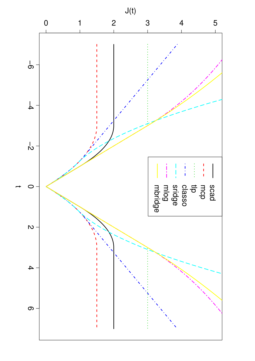
is concave function, where $\kappa_{\lambda}=\lim_{t\to 0+}\nabla J_{\lambda}(t)$. The class includes most of existing non-convex penalties: SCAD (Fan and Li 2001),

$$\nabla J_{\lambda}(t)=\lambda I[0<t<\lambda]+\{(\tau\lambda-t)/(\tau-1)\}I[\lambda\leq t<\tau\lambda]$$

for $\tau>2$, MCP (Zhang 2010),

$$\nabla J_{\lambda}(t)=(\lambda-t/\tau)I[0<t<\tau\lambda]$$

for $\tau>1$, truncated $\ell_{1}$-penalty (Shen et al. 2013),

$$\nabla J_{\lambda}(t)=\lambda I[0<t<\tau]$$

for $\tau>0$, moderately clipped LASSO (Kwon et al. 2015),

$$\nabla J_{\lambda}(t)=(\lambda-t/\tau)[0<t<\tau(\lambda-\gamma)]+\gamma[t\geq\tau(\lambda-\gamma)]$$

for $\tau>1$ and $0\leq\gamma\leq\lambda$, sparse ridge (Kwon et al. 2013),

$$\nabla J_{\lambda}(t)=(\lambda-t/\tau)I[0<t<\tau\lambda/(\tau\gamma+1)]+\gamma tI[t\geq\tau\lambda/(\tau\gamma+1)]$$

for $\tau>1$ and $\gamma\geq 0$, modified log (Zou and Hastie 2005b).

$$\nabla J_{\lambda}(t)=(\lambda/\tau)[0<t<\tau]+(\lambda/t)[t\geq\tau]$$

for $\tau>0$, and modified bridge (Huang et al. 2008)

$\displaystyle\nabla J_{\lambda}(t)=(\lambda/2\sqrt{\tau})[0<t<\tau]+(\lambda/2\sqrt{t})[t\geq\tau]$

for $\tau>0$.

The moderately clipped LASSO and sparse ridge are simple smooth interpolations between the MCP (near the origin) and the LASSO and ridge, respectively. The log and bridge penalties are modified to be linear over $t\in(0,\tau]$ so that they have finite right derivative at the origin. See the plot for graphical comparison of the penalties introduced here.

The CCCP-MLQA algorithm iteratively conducts two main steps: CCCP (Yuille and Rangarajan 2003) and MLQA (Lee et al. 2016) steps. The CCCP step decomposes the penalty $J_{\lambda}$ as in (2) and then minimizes the tight convex upper bound obtained from a linear approximation of $D_{\lambda}$. The MLQA step first minimizes a quadratic approximation of the loss $L$ and then modifies the solution to keep descent property.

Usually, the computation time of the algorithm rapidly increases as the number of non-zero parameters increases or $\lambda$ decreases toward zero. To accelerate the algorithm, we incorporate the active-set-control procedure while constructing the solution path over a decreasing sequence of $\lambda$.

Assume that $\lambda$ is given and we have an initial solution $\tilde{\mbox{\boldmath{$\beta$}}}$ which is expected to be very close to the minimizer of $Q_{\lambda}(\mbox{\boldmath{$\beta$}})$. First we check the first order KKT optimality conditions:

$$\partial Q_{\lambda}(\tilde{\mbox{\boldmath{$\beta$}}})/\partial\beta_{j}=0,j\in{\cal A}~~\mbox{and}~~|\partial Q_{\lambda}(\tilde{\mbox{\boldmath{$\beta$}}})/\partial\beta_{j}|\leq\kappa_{\lambda},j\in{\cal N},$$

(6)

where ${\cal A}=\{j:\tilde{\beta}_{j}\neq 0\}$ and ${\cal N}=\{j:\tilde{\beta}_{j}=0\}$. We stop the algorithm if the conditions are satisfied else update ${\cal N}$ and $\tilde{\mbox{\boldmath{$\beta$}}}$ by ${\cal N}={\cal N}\setminus\{j_{\max}\}$ and

$$\tilde{\mbox{\boldmath{$\beta$}}}={\arg\min}_{\beta_{j}=0,j\in{\cal N}}Q_{\lambda}(\mbox{\boldmath{$\beta$}}),$$

(7)

respectively, where $j_{\max}={\arg\max}_{j\in{\cal N}}|\partial Q_{\lambda}(\tilde{\mbox{\boldmath{$\beta$}}})/\partial\beta_{j}|$. We keep these iterations until the KKT conditions in (6) are satisfied with $\tilde{\mbox{\boldmath{$\beta$}}}$. The key step is (7) which is easy and fast to obtain by using Algorithm 1 and 2 since the objective function only includes the parameters in ${\cal A}\cup\{j_{\max}\}$.

The option alpha in the main functions forces the algorithm to solve the following penalized problem with the $\ell_{2}$-regularization or ridge effect (Zou and Hastie 2005b).

$$Q_{\lambda}(\mbox{\boldmath{$\beta$}})=\frac{1}{n}\sum_{i=1}^{n}\ell_{i}(\mbox{\boldmath{$\beta$}})+\alpha\sum_{j=1}^{p}J_{\lambda}(|\beta_{j}|)+(1-\alpha)\lambda\sum_{j=1}^{p}\beta_{j}^{2},$$

(8)

where $\alpha\in[0,1]$ is the value from the option alpha, which is the mixing parameter between the penalties $J_{\lambda}$ and ridge. The objective function in (8) includes the elastic net (Zou and Hastie 2005b) when $J_{\lambda}(t)=\lambda t$ and Mnet (Huang et al. 2016) when $J_{\lambda}(\cdot)$ is the MC penalty. By controlling the option alpha, we can treat the problem with highly correlated variables, and it also makes the algorithm more stable.

We can give different weights for each observation and penalty by the options obs.weight and pen.weight, which provides the minimizer of

$$Q_{\lambda}(\mbox{\boldmath{$\beta$}})=\sum_{i=1}^{n}d_{i}\ell_{i}(\mbox{\boldmath{$\beta$}})+\sum_{j=1}^{p}w_{j}J_{\lambda}(|\beta_{j}|),$$

(9)

where $d_{i}$ is the weight for the $i$th observation and $w_{j}$ is the penalty weight for the $j$th variable. For example, controlling observation weights is required for the linear regression model with heteroscedastic error variance. Further, we can compute adaptive versions of penalized estimators by giving different penalty weights as in the adaptive LASSO (Zou 2006).

It is common practice to standardize variables prior to fitting the penalized models, but one may opt not to. Hence, we provide the option x.standardize for flexible analysis. The option x.standardize=TRUE means that the algorithm solves the original penalized problem in (1), with the standardized (scaled) variables, and then the resulting solution $\hat{\beta}_{j}$ is converted to the original scale by $\hat{\beta}_{j}/s_{j}$, where $s_{j}=\sum_{i=1}^{n}x_{ij}^{2}/n$. When the penalty $J_{\lambda}$ is the LASSO penalty, this procedure is equivalent to solving following penalized problem

$$Q^{s}_{\lambda}(\mbox{\boldmath{$\beta$}})=L(\mbox{\boldmath{$\beta$}})+\sum_{j=1}^{p}\lambda_{j}|\beta_{j}|,$$

where $\lambda_{j}=\lambda s_{j}$, which is another adaptive version of the LASSO being different from the adaptive LASSO (Zou 2006).

We introduced the warm start strategy for speed up the algorithm, but the solution path, in fact, depends on the initial solution of the CCCP algorithm because of the non-convexity. The option local=TRUE in ncpen provides the same initial value specified by the option local.initial into each CCCP iterations for whole $\lambda$ values. The use of the option local=TRUE makes the algorithm slower but the performance of the resulting estimator would be often improved as provided a good initial such as the maximum likelihood estimator or LASSO.

The package ncpen includes several user-friendly functions such as cv.ncpen that conducts the cross-validation to select an optimal tuning parameter $\lambda$. In addition, the function gic.ncpen calculates theoretically optimal $\lambda$ based on the generalized information criterion (Wang et al. 2007; Wang et al. 2009; Fan and Tang 2013; Wang et al. 2013).

We consider the linear and logistic regression models to calculate the total elapsed time for constructing the solution path over 100 $\lambda$ values:

$$y={\bf x}^{T}\mbox{\boldmath{$\beta$}}^{*}+\varepsilon~~\mbox{and}~~\mathbb{P}(y=1|{\bf x})=e^{{\bf x}^{T}\mbox{\scriptsize\boldmath{$\beta$}\unboldmath}}/(1+e^{{\bf x}^{T}\mbox{\scriptsize\boldmath{$\beta$}\unboldmath}})$$

(10)

where ${\bf x}\sim N_{p}(\mathbf{0},\Sigma)$ with $\Sigma_{jk}=0.5^{|j-k|}$, $\beta_{j}=1/j$ for $j,k=1,\cdots,p$ and $\varepsilon\sim N(0,1)$. The averaged elapsed times of ncpen in 100 random repetitions are summarized in Table 1 and 2 for various $n$ and $p$, where the penalties are the SCAD, MCP, truncated $\ell_{1}$ (TLP), moderately clipped LASSO (CLASSO), sparse ridge (SR), modified bridge (MBR) and log (MLOG). For comparison, we try ncvreg for the SCAD also. The results show that all methods in ncpen are feasible for high-dimensional data.

We compare the solution paths based on the diabetes samples available from lars package (Efron et al. 2004), where the sample size $n=442$ and the number of covariates $p=64$, including quadratic and interaction terms. Figure 2 shows four plots where the top two panels draw the solution paths from the LASSO and SCAD with $\tau=3.7$ given by ncvreg and bottom two panels draw those from the SCAD with $\tau=3.7$ based on ncpen with and without standardization of covariates. Two solution paths from ncvreg and ncpen with standardization are almost the same since ncvreg standardizes the covariates by default, which is somewhat different from that of ncpen without standardization. Figure 3 shows the solution paths from six penalties with standardization by default in ncpen: the MCP, truncated $\ell_{1}$, modified log, bridge, moderately clipped LASSO and sparse ridge.

There are cases when we need to introduce the ridge penalty for some reasons, and ncpen provides a hybrid version of the penalties: $\alpha J_{\lambda}(|t|)+(1-\alpha)|t|^{2}$, where $\alpha$ is the mixing parameter between the penalty $J_{\lambda}$ and ridge effects. For example, the non-convex penalties often produce parameters that diverge to infinity for the logistic regression because of perfect fitting. Figure 4 shows the effects of ridge penalty where the leukemia samples in plsgenomics are used for illustration. The solution paths using the top 50 variables with high variances are drawn when $\alpha\in\{1,0.7,0.3,0\}$ for the SCAD and modified bridge penalties. The solution paths without ridge effect ($\alpha=1$) tend to diverge as $\lambda$ decreases and become stabilized as the ridge effect increases ($\alpha\downarrow$ ).

We introduced the warm start strategy for speed up the algorithm but the solution path, in fact, depends on the initial solution because of the non-convexity. For comparison, we use the leukemia samples and the results are displayed in Figure 5 and Table 3. In the figure, left panels show the solution paths for the SCAD, MCP and clipped LASSO obtained by the warm start, and the right panels show those obtained by using the LASSO as a global initial for the CCCP algorithm. Figure 5 shows two strategies for initial provide very different solution paths, which may result in different performances of the estimators. We compare the prediction accuracy and selectivity of the estimators by two strategies. The results are obtained by 300 random partitions of data set divided into two parts, training (90%) and test (10%) datasets. For each training data, the optimal tuning parameter values are selected by 10-fold cross-validation, and then we compute the prediction error on each test datasets and the number of selected nonzero variables. Table 3 shows all methods by the global initial perform better than those by the warm start strategy. In summary, the nonconvex penalized estimation depends on the initial solution, and the non-convex penalized estimator by a good initial would improve its performance.

References

- Breheny and Huang (2011) Breheny, P. and Huang, J. (2011). Coordinate descent algorithms for nonconvex penalized regression, with applications to biological feature selection. Ann. Appl. Stat., 5 232.
- Eddelbuettel et al. (2011) Eddelbuettel, D., François, R., Allaire, J., Ushey, K., Kou, Q., Russel, N., Chambers, J. and Bates, D. (2011). Rcpp: Seamless r and c++ integration. Journal of Statistical Software, 40 1–18.
- Efron et al. (2004) Efron, B., Hastie, T., Johnstone, I., Tibshirani, R. et al. (2004). Least angle regression. Ann. Stat., 32 407–499.
- Fan and Li (2001) Fan, J. and Li, R. (2001). Variable selection via nonconcave penalized likelihood and its oracle properties. J. Am. Stat. Assoc., 96 1348–1360.
- Fan and Tang (2013) Fan, Y. and Tang, C. Y. (2013). Tuning parameter selection in high dimensional penalized likelihood. Journal of the Royal Statistical Society: Series B (Statistical Methodology), 75 531–552.
- Friedman (2012) Friedman, J. (2012). Fast sparse regression and classification. International Journal of Forecasting, 28 722–738.
- Friedman et al. (2007) Friedman, J., Hastie, T., Höfling, H., Tibshirani, R. et al. (2007). Pathwise coordinate optimization. The Annals of Applied Statistics, 1 302–332.
- Friedman et al. (2010) Friedman, J., Hastie, T. and Tibshirani, R. (2010). Regularization paths for generalized linear models via coordinate descent. J. Stat. Softw., 33 1.
- Huang et al. (2016) Huang, J., Breheny, P., Lee, S., Ma, S. and Zhang, C. (2016). The mnet method for variable selection. Statistica Sinica. DOI, 10.
- Huang et al. (2013) Huang, J., Breheny, P., Lee, S., Ma, S. and Zhang, C.-H. (2013). Balancing stability and bias reduction in variable selection with the mnet estimator. Statistica Sinica, 1081.
- Huang et al. (2008) Huang, J., Horowitz, J. L. and Ma, S. (2008). Asymptotic properties of bridge estimators in sparse high-dimensional regression models. The Annals of Statistics 587–613.
- Jiang and Huang (2014) Jiang, D. and Huang, J. (2014). Majorization minimization by coordinate descent for concave penalized generalized linear models. Statistics and computing, 24 871–883.
- Kim et al. (2008) Kim, Y., Choi, H. and Oh, H.-S. (2008). Smoothly clipped absolute deviation on high dimensions. Journal of the American Statistical Association, 103 1665–1673.
- Kim and Kwon (2012) Kim, Y. and Kwon, S. (2012). Global optimality of nonconvex penalized estimators. Biometrika, 99 315–325.
- Kwon and Kim (2012) Kwon, S. and Kim, Y. (2012). Large sample properties of the scad-penalized maximum likelihood estimation on high dimensions. Statistica Sinica 629–653.
- Kwon et al. (2013) Kwon, S., Kim, Y. and Choi, H. (2013). Sparse bridge estimation with a diverging number of parameters. Statistics and Its Interface, 6 231–242.
- Kwon et al. (2015) Kwon, S., Lee, S. and Kim, Y. (2015). Moderately clipped lasso. Computational Statistics & Data Analysis, 92 53–67.
- Lee (2015) Lee, S. (2015). A note on standardization in penalized regressions. Journal of the Korean Data and Information Science Society, 26 505–516.
- Lee et al. (2016) Lee, S., Kwon, S. and Kim, Y. (2016). A modified local quadratic approximation algorithm for penalized optimization problems. Computational Statistics & Data Analysis, 94 275–286.
- Mazumder et al. (2011) Mazumder, R., Friedman, J. H. and Hastie, T. (2011). Sparsenet: Coordinate descent with nonconvex penalties. Journal of the American Statistical Association, 106 1125–1138.
- Park and Hastie (2007) Park, M. Y. and Hastie, T. (2007). L1-regularization path algorithm for generalized linear models. Journal of the Royal Statistical Society: Series B (Statistical Methodology), 69 659–677.
- Shen et al. (2012) Shen, X., Pan, W. and Zhu, Y. (2012). Likelihood-based selection and sharp parameter estimation. Journal of the American Statistical Association, 107 223–232.
- Shen et al. (2013) Shen, X., Pan, W., Zhu, Y. and Zhou, H. (2013). On constrained and regularized high-dimensional regression. Annals of the Institute of Statistical Mathematics, 65 807–832.
- Tibshirani (1996) Tibshirani, R. (1996). Regression shrinkage and selection via the lasso. Journal of the Royal Statistical Society. Series B (Methodological) 267–288.
- Tseng (2001) Tseng, P. (2001). Convergence of a block coordinate descent method for nondifferentiable minimization. Journal of optimization theory and applications, 109 475–494.
- Wang et al. (2009) Wang, H., Li, B. and Leng, C. (2009). Shrinkage tuning parameter selection with a diverging number of parameters. Journal of the Royal Statistical Society: Series B (Statistical Methodology), 71 671–683.
- Wang et al. (2007) Wang, H., Li, R. and Tsai, C.-L. (2007). Tuning parameter selectors for the smoothly clipped absolute deviation method. Biometrika, 94 553–568.
- Wang et al. (2013) Wang, L., Kim, Y. and Li, R. (2013). Calibrating non-convex penalized regression in ultra-high dimension. Annals of statistics, 41 2505.
- Yuille and Rangarajan (2003) Yuille, A. and Rangarajan, A. (2003). The concave-convex procedure. Neural Computation, 15 915–936.
- Zhang (2010) Zhang, C. (2010). Nearly unbiased variable selection under minimax concave penalty. Ann. Stat., 38 894–942.
- Zhang and Zhang (2012) Zhang, C.-H. and Zhang, T. (2012). A general theory of concave regularization for high-dimensional sparse estimation problems. Statistical Science 576–593.
- Zou (2006) Zou, H. (2006). The adaptive lasso and its oracle properties. Journal of the American statistical association, 101 1418–1429.
- Zou and Hastie (2005a) Zou, H. and Hastie, T. (2005a). Regularization and variable selection via the elastic net. Journal of the Royal Statistical Society: Series B (Statistical Methodology), 67 301–320.
- Zou and Hastie (2005b) Zou, H. and Hastie, T. (2005b). Regularization and variable selection via the elastic net. J. Roy. Stat. Soc. B, 67 301–320.
- Zou and Li (2008) Zou, H. and Li, R. (2008). One-step sparse estimates in nonconcave penalized likelihood models. Annals of statistics, 36 1509.