Monte Carlo simulation of cosmologies with dust
Abstract
The quantum theory of the Friedmann cosmological model with dust and cosmological constant () is not exactly solvable analytically. We apply Path Integral Monte Carlo (PIMC) techniques to study its quantum dynamics using the physical Hamiltonian corresponding to the dust field as a clock. We study (i) quantum fluctuations around classical paths and (ii) formulate the analogues of the no-boundary and tunnelling proposals and simulate the ground state wave functions. For a unique ground state wave function exists. For the physical Hamiltonian is not bounded below, but the path integral for the propagator is convergent over a range of Euclidean time . We investigate the properties of the convergent propagator. The path integral can be made convergent for all values of by restricting the integral over paths with action greater than equal to zero. We explore the consequences of such a choice.
I Introduction
The problem of quantizing gravity is one at the forefront of theoretical physics. Studies of quantum effects in gravity began soon after the completion of General Relativity (GR), and continues to the present time, spanning almost a century Rovelli 2000. Despite this, at present there is no consensus on a theory of quantum gravity, although there are multiple competing ideas. These include Causal Dynamical Triangulations (CDT), Causal Sets, Loop Quantum Gravity (LQG), Asymptotic Safety, Euclidean Quantum Gravity and String Theory (– see e.g. Carlip et al. 2017 for an overview of some of these approaches).
Within the context of canonical quantization, the path integral approach may be utilized to find solutions to the Wheeler DeWitt (WDW) equation. Specifying solutions to the WDW equation involves choosing appropriate boundary conditions for the equation i.e, prescribing the initial conditions for the universe. In the sum over histories approach this corresponds to the choice of paths (or histories) to be included in the sum. It was demonstrated by Hartle and Hawking that the amplitude for a particular -geometry can be obtained via a semiclassical evaluation of the sum over all -geometries it bounds Hartle and Hawking 1983. This is the “no boundary proposal.” Several proposals have since been made for both the boundary conditions and the set of paths to be included in the sum to find solutions of the WDW Vilenkin 1982; Vilenkin 1986; Halliwell and Louko 1989; Halliwell and Hartle 1990; Feldbrugge et al. 2017. However, these proposals have all been restricted to semiclassical approximations of the path integral.
Aside from technical difficulties in obtaining a computable theory of quantum gravity, there are conceptual challenges as well. One notable issue is the problem of time Isham 1992. Evolution in quantum theory requires a fixed notion of time, external to the physical system under study. This is the set of times corresponding to Galilean inertial frames in non-relativistic quantum theory, and the set corresponding to Lorentzian inertial observers in relativistic quantum theory on Minkowski spacetime. In both these cases time is provided by a fixed external kinematical structure, the space(time) metric. In general relativity there are no fixed metrics, and any notion of time must be found within the system. This is the problem of time.
One way to avoid this issue in canonical quantum gravity is to use an (arbitrary) reference time, whereby a phase space variable is chosen as a clock, and the evolution of all other phase space variables is with respect to this choice; the Hamiltonian constraint of general relativity is solved classically for the momentum conjugate to the chosen time function to obtain the corresponding (non-vanishing) physical Hamiltonian. Quantization then proceeds by promoting this physical Hamiltonian to an operator on a suitable Hilbert space. This method, called deparametrization, leads to the reduced phase space of physical degrees of freedom.
Reduced physical Hamiltonians arising from general relativity are not easy to quantize, except in very special cases. Furthermore, the theories resulting from different time choices are in general not unitarily equivalent, and different from Dirac quantization (see e.g. Schleich 1990), where the Hamiltonian constraint is imposed as an operator condition. (There is however at least one example in which the results are equivalent for a particular choice of operator ordering in the Dirac quantization scheme Maeda 2015; Ali et al. 2018.)
Despite these issues, there has been recent focus on numerical simulations in order to bypass the difficulties of performing analytical calculations in the various approaches to quantum gravity. Several approaches utilize a sum over histories formulation for the dynamics, each differing in discretization schemes. Notable examples include CDT Ambjorn et al. 2010, causal sets Rideout and Sorkin 2000, and spin foams Perez 2013. In addition to making the problem of quantum gravity tractable, numerical simulations within these approaches have provided potentially useful insights into the quantum nature of gravitation Ambjorn et al. 2005; Glaser and Surya 2016.
Here we are interested in exploring the path integral approach numerically within the framework of canonical quantum gravity, with specific application to cosmology, using a matter time gauge. We propose a method to study the reduced phase space quantization of a closed FLRW universe with non-zero and a dust field. This system has no exact solution in quantum theory, except for zero curvature Husain and Pawlowski 2011; Ali et al. 2018. We use the dust field as an internal clock, and the corresponding physical Hamiltonian to define a path integral. We then use PIMC techniques to study the quantum theory. Although the study of a particular mini-superspace model does not amount to the study of a full theory of quantum gravity, it provides a testbed for polishing tools and perhaps inferring some qualitative features of the complete theory. We emphasize that although FRLW quantum cosmology has been studied in several different ways, the cases we consider have no exact analytic solutions – all results to date are either semi-classical or other approximations, including in Loop Quantum Cosmology Agullo and Singh 2017. Therefore the quantum theory of this model with matter is useful to study using PIMC.
Monte-Carlo methods are a staple tool in many areas of physics (e.g. lattice QCD Gattringer and Lang 2010 and atomic and nuclear physics). In the context of quantum cosmology, these methods have been applied to cosmological models Berger 1988; Berger 1989; Berger 1993. For example Ref. Berger 1993 contains a study of ansätze for regulating the path integral for mini-superspace models, where the Hamiltonian constraint is not solved classically (although the lapse () is fixed using the condition ). Our approach is different in that we deparmetrize first, and then use the resulting physical Hamiltonian for simulations. Furthermore, in contrast to the pure deSitter models studied in literature Berger 1993; Halliwell and Louko 1989 our model retains a physical degree of freedom after gauge fixing.
The outline of the paper is as follows. In Section II we define the model and the associated path integral. In Section III we review the PIMC method and detail the Metropolis algorithm as applied to the system under study. In Sections IV, V and VI, we provide details of our simulations and results. We conclude in Section VII with a summary of our main results and the prospects for further study of canonical quantum gravity models using similar methods. (Throughout we work in units with .)
II The Model
The action of the theory we study is
| (1) |
where is the dust field, and is its energy density. The corresponding canonical action is
| (2) | |||||
where
| (3) |
Here () and () are the gravitational and dust degrees of freedom respectively, and is the lapse and is the shift.
We proceed by using the dust field to fix the time gauge Husain and Pawlowski 2012; Husain and Pawlowski 2011. We set with and solve the Hamiltonian constraint () for the conjugate momentum to the dust field. The physical Hamiltonian is then given by
| (4) |
Requiring that the gauge be preserved in time fixes the lapse to . For now we leave the sign of the lapse undetermined, but we will fix it later; the sign of the lapse determines how the dust energy density () relates to the physical Hamiltonian: negative lapse corresponds to a positive dust energy density when Ali et al. 2016; Hassan and Husain 2017.
This paper is concerned with the homogeneous isotropic cosmological metrics
| (5) |
where is the spatial curvature. In these coordinates, where the spatial metric is conformally flat, the canonical theory in the dust time gauge takes a simple form. Let us define , , , and set
| (6) |
where we take the reduced phase space to be . The various factors ensure that .
This is an unconventional canonical parametrization where . It has the advantage that the gravitational kinetic term is proportional to , and the physical Hamiltonian in the dust time gauge takes the form
| (7) |
(after the rescalings , ). The corresponding action is
| (8) |
For , Eq. (8) becomes the action of a particle moving in the potential
| (9) |
This is the choice we make. The case is then a simple harmonic oscillator for , and an inverted oscillator for Ali et al. 2018. For non-zero the equation of motion is
| (10) |
This is singular at . Fig. 1 displays the phase portraits for typical values of . The case exhibits two saddle points where ; near these points the trajectory flow lines on either side are toward or away from the singularity at .
We are interested in computing the path integral
| (11) |
for the action (8), with and As for all such integrals, this is oscillatory and so difficult to evaluate. We therefore do a Wick rotation in the dust time gauge: . This converts Eq. (11) to
| (12) |
where
| (13) |
This integral is not analytically tractable for . We therefore proceed by numerically computing the path integral using a Monte Carlo method. In the following section we define this process in detail.
III Monte Carlo method
We propose to evaluate the integral (12) using the Path Integral Monte Carlo (PIMC) technique. The central idea is to generate representative sets of paths that are then weighed with action to calculate the integral.
As is well known, in classical theory there is a unique on shell-path once the initial conditions are specified, whereas in quantum theory an infinite number of paths contribute to the Feynman path integral, each with a phase . After Wick rotation, the amplitude may be treated as a probability distribution on the space of paths. The PIMC technique generates a Markov chain of paths from an initial seed path, such that the stationary distribution for the Markov chain is given by the amplitude . In order to probe the space of paths effectively we use the Metropolis algorithm for importance sampling. In this approach paths with large positive are suppressed.
We start by discretizing the action (13). The time interval from to is divided into steps; . For the time-derivative, we use a forward step, . The corresponding discrete action is
| (14) |
With this discretization, the MCMC method we use proceeds as follows. After fixing an initial path , (which could be selected by a deterministic or random rule),
- 1.
Change a random element of the array: , where is a random number chosen from a uniform distribution, with a fixed parameter;
- 2.
Calculate the change in the Euclidean action: ;
- 3.
Accept or reject this change. If , the change is accepted, otherwise it is accepted with a probability ; if accepted, the selected element is updated: ;
- 4.
Repeat times the steps . This defines one Monte Carlo (MC) iteration.
An important element in each run is thermalization. This consists of performing a number of MC steps until the action is thermalized. This is to ensure that the MCMC process has lost memory of the starting point before sample path selection begins. is chosen so that the order parameter used (the Euclidean action in our case) reaches an equilibrium value, up to small fluctuations. Fig. 2 shows the thermalization of the action for a representative run for a given set of MC parameters, with various . It is evident that the action converges to approximately the same value.
Once thermalization is complete, a number of MC steps is carried out. Paths are selected as part of the sample every steps, a number determined so as to reduce autocorrelations. After a sufficient number of sample paths are gathered through this process, computation of propagators and expectation values of observables can proceed.
At this stage, it is important to note a key difference between the cosmology we are studying and conventional quantum mechanical systems: The potential (9) is not bounded below when either , or , or both. Thus the Hamiltonian is not bounded below and the Euclidean path integral does not appear to converge. We consider two methods to deal with this issue:
1. Convergence of path integrals of systems with Hamiltonians unbounded below were investigated in Carreau et al. 1990, with the conclusion that for potentials diverging at most as , the path integral is convergent if the Euclidean time is less than . The argument is worth summarizing as it applies directly to our system. Let denote the kinetic term in Eq. (12). Then
| (15) | |||||
where max denotes the maximum value of along each path between and ; the last inequality follows since including the term reduces the integral. To further constrain the r.h.s., we must bound the expectation value with the weight to include all paths between and (in time ) that exceed the value . This requires an integration over from to . This is accomplished by noting the following: (i) The amplitude from to in time with respect to the free action is , (ii) by the reflection principle, for paths crossing , , (iii) the amplitude for all paths that lie between and is therefore . Using this last expression to compute , we arrive at the bound
| (16) |
The integral in the last inequality is convergent if , and thus is bounded for all .
We use this result to calculate the amplitude for the universe to expand from nearly zero volume to some finite volume in section IV. In sections V and VI, though we do not fix the end point we find the integral is convergent for some values of . We calculate the no boundary wave function and the tunnelling wave function for these values.
2. An alternative way to proceed is by restricting the integral to the set of paths on which the Euclidean action is manifestly positive or zero. (This is similar to the approach in Berger 1993 where the vacuum model was studied without solving the Hamiltonian constraint classically). This is motivated by the duality between Euclidean quantum field theory and statistical mechanics (see e.g. McCoy 1994): The Euclidean action of the quantum theory is akin to the Hamiltonian of a stat-mech system with time identified as (inverse) temperature (),
| (17) |
Requiring that this Hamiltonian (our Euclidean action) be positive,
| (18) |
fixes the ground state at and yields a convergent integral.
A necessary consequence of this regularization is that for (or ) there is no unique ground state. In fact an infinite number of degenerate vacua exist since there is an uncountably infinite number of paths which yield . Thus the physical results depend quantitatively on whichever subset of vacua the MCMC process converges to in each run. However despite this ambiguity, there are qualitative features common to different vacua which we explore in the following sections; we can compare the averages of observables calculated over different subsets of vacua to extract common features11 1 This situation with infinite degenerate vacua can be compared to another physical system: A particle in a Mexican hat potential: , where there is also a one-parameter infinite degeneracy of vacua labeled by the angle . Nonetheless, in this case there is an observable whose value is invariant for all the vacua; this is the radial co-ordinate ; depending on the potential its expectation value is constant. All other observables, such as , take on different random values on the different vacua. In our case however, there is no such ‘invariant observable’ apart from the action itself.. Note that for and , a unique vacuum does exist.
IV Semiclassical calculations
Although PIMC is capable of performing non-perturbative calculations, it is useful to also look at semiclassical theory to see if intuitions are borne out. In this section, we will look at quantum fluctuations around specific classical solutions for which . The equation of motion in Euclidean time is
| (19) |
For , this equation cannot be solved analytically so a classical solution must be generated numerically. For this we restrict attention to small initial Universes. Numerically this means choosing where is a small positive number, since the point is singular.
The Monte Carlo process is seeded initially by the classical solution, with the end points and held fixed. We computed the mean path , and fluctuations in volume for three sets of parameter values . The results are shown in Fig. 3 and Fig. 4. The figures show that (i) the average quantum path does not deviate too far away from the classical path, and (ii) the relative volume fluctuations are large when the Universe is small, and gradually die off as the Universe expands. These results are in accord with expectations, and so provide some verification of our method. Let us however note that the deviation between the classical and semi-classical path is largest for the case . This is understood by considering the shape of the potential (9) for various parameter values: for the first and last frames in Fig. 3, the width of the potential barrier connecting the smaller and larger values of is significantly larger than for the center frame. Thus the probability of tunnelling to larger values, is much larger for the center frame, hence the larger deviation from classicality for .
V No-Boundary wave function
The no boundary wave function is given by the path integral
| (20) |
where the integral is over all compact -geometries bounded by a -geometry with induced metric Hartle and Hawking 1983. Since compact geometries are summed over, this integral may be interpreted as the amplitude for the -geometry to arise from “nothing,” i.e a zero -geometry or a point. In our model with dust, the no boundary proposal would correspond to calculating the amplitude of a finite spatial volume -geometry to arise from a zero volume one. That is, we integrate over sets of paths with , with the final value left unspecified; the wave function we calculate is
| (21) |
This proposal is similar to the prescription in Louko 1988 given in canonical coordinates. It may still be considered as a “no-boundary” wave function, despite the following differences from the original Hartle-Hawking (HH) proposal: (i) We fix a time gauge and solve the Hamiltonian constraint right at the outset – there is no integration over the lapse function; we are not seeking solutions of the Wheeler DeWitt equation. (ii) A fixed time gauge also implies that the proper time and the foliation between the initial and final hypersurfaces are fixed. Thus we are integrating over geometries between these hypersurfaces and not over arbitrary geometries as in the HH proposal. (iii) As in the Euclidean path integral approach, the integral we consider is also unbounded. However, unlike the HH calculation, the PIMC gives the full path integral and not a saddle point approximation. Let us note that we consider here only the boundary condition , and leave to be determined randomly by the (random) choice of the second value in the path array, ; it is of course possible to also fix by fixing the value of via the prescription , and then randomly selecting the rest of the path. This fixing of two path elements (instead of one) will not make a significant difference to our results for sufficiently long or finely discretized paths.)
As described in the previous section Eq. (V) is discretized as
where the sample paths include only those with and left free. The wavefunction is determined by binning the values of at the last time step . We consider the two distinct cases and .
V.1
For this case the Euclidean action is bounded below so a unique ground state exists. In the large limit the PIMC algorithm converges to this ground state. The action stabilizes at a finite positive value. Our results appear in Fig. 5 and Fig. 6.
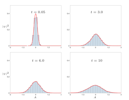
All plots in Fig. 5 are for a fixed final time in the path integral. It displays snapshots of the wave function at various , obtained by binning paths on the indicated fixed slices. It is evident that the wave function starts out highly peaked at for small and spreads as increases. The runs from which these plots were made were initiated with a random initial path with , , and parameter values , and .
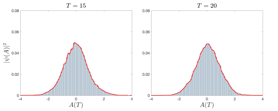
Fig. 6 shows the same wave function but at only the final time in the path integral, , for and . It is evident from this that the results are almost identical, indicating a stable late time wave function. These plots were again produced from PIMC runs with a random initial path with and , but this time with , , , and a bin size of .

Lastly for this case, since the ground state is unique, we can calculate the two point correlation function in the state in the usual way by computing
| (22) |
This is just the MC average of . Fig. 7 shows the correlation functions and as functions of for . For comparison, it is worth noting that the volume correlator was also recently computed in the context of the CDT program for and toroidal spatial slices Knorr and Saueressig 2018, where the emergent metric is of the FRW form; this work indicates an exponential decay forward in time, similar to what we find here. It is curious that this occurs despite the fact that, unlike in CDT, we simulate the classically symmetry reduced theory.
V.2
In this case the Euclidean action is not bounded below, but as discussed above, the path integral is convergent for . (For the presently observed value of , this is in fact very large.)
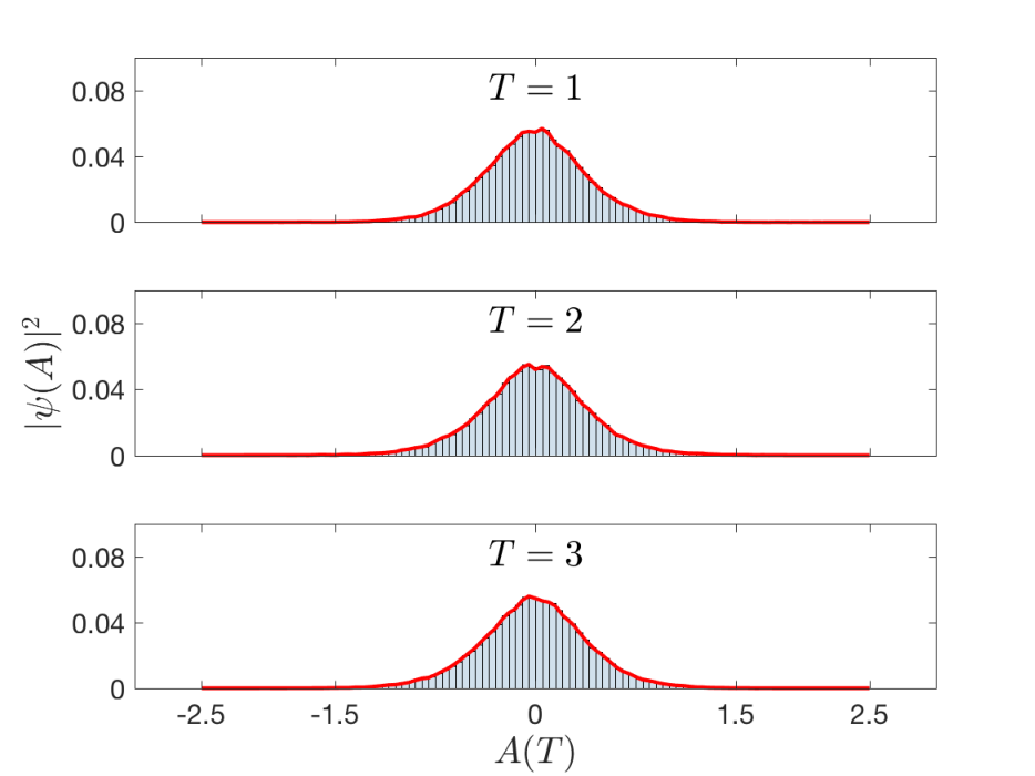
For such values of we can compute the no-boundary wave function Eq. (V). Fig. 8 shows the results for , and computed using samples from independent simulations. The samples were collected after different numbers of thermalization sweeps. The actions for the samples collected after thermalization sweeps and thermalization sweeps are quite similar, both in value and the rate of change, and both appear to be sufficiently thermalized. However, the wave functions computed from these samples are different. After thermalization sweeps, several sample paths appear to take on large values whereas after thermalization sweeps the second peak at large disappears. The tails of the distribution after the thermalization sweeps are significantly thicker compared to the distribution after million sweeps. We tested up to million thermalization steps and found that after approximately 1.5 million steps, the slope in the action as a function of time did not change significantly. This is an indication that thermalization in fact did occur. (The cost of our algorithm is order where is the path array size, so the growth in time cost is linear.) Thus, even though the action thermalizes slowly, the trend in Fig. 8 suggests that universes of large volume are less probable, at least for these values of and .
It is interesting to compare the last plot in Fig. 8 with the plots in Fig. 9 which shows the no boundary wave function at different values of with parameters and . All three plots in Fig. 9 indicate that the universe does not expand to very large volumes within the interval of convergence for the path integral. However, the tails of the wavefunction for , in Fig. 8 are nearly twice as long as the tails for the wave functions in Fig. 9. Fig. 10 compares the wavefunctions for for both cases. This comparison suggests that larger universes are more probable for smaller values of .
As discussed above, an alternatively method for exploring the path integral that is convergent for all is to use only those paths for which . In general, the set of paths yielding is uncountably infinite, and the fraction of classical paths in this set is very small. This is displayed in Fig. 12.

In a single MC run only a subset of the paths can be explored. The size and characteristics of this subset are determined by the initial path provided to the algorithm, and the parameter . As there is no unique ground state, (since numerous physically different configurations have ), the surface defines a continuum of vacua. The PIMC algorithm then converges rapidly to the nearest accessible subset of vacua in each run.
Fig. 12 shows the expectation value of volume as a function of time for four different MC runs. Each run was started with a randomly selected initial path and the same value of , and . The common feature in the runs is that the volume of the universe is a non-monotonic function of time. In contrast with Figs. 8 and 9, large volumes do arise for initial paths entered starting from zero volume, at least for some period of time. However, each run results in a different trajectory.
Thus, we see that the two distinct ways of computing the no-boundary wave function we have explored, namely restricting final time to obtain a convergent result on the one hand, and setting on the other, give different physical predictions. The former method is stable and convergent for very small (compatible with observations), whereas the latter gives predictions results that are entirely dependent on the initial state due to the large vacuum degeneracy give by the bound.
VI Tunnelling wave function

The PIMC method we are studying may also be used to calculate tunelling wave functions Vilenkin 1986; Vilenkin 1988. The proposal is basically that the wave function of the universe include only outgoing waves at the “boundaries” of superspace. A concrete formulation for this proposal for a deSitter model with a scalar field appears in Vilenkin 1994.
We propose here a slightly different notion of tunnelling tailored to our calculation method, and in line with the conventional definition of tunnelling in quantum mechanical systems. This is illustrated in Fig. 14. The potential (9) with has two maxima (). We wish to calculate the wave function for paths with some fixed total energy that start with some small value of within the classically allowed region, and tunnel into the potential barrier beyond the classical turning points within some time . Since the rejection rates of the MC simulations for paths with fixed energy are quite high, we consider paths in some energy band . These paths are colored blue in Fig. 14 and are the analogue of the outgoing modes in Vilenkin’s proposal.
The algorithm for the simulation is the same as described in Section III except that all paths with pointwise energy outside the band are rejected. Another difference in these simulations is that a symmetric discretization is used for the potential as compared to the pointwise discretization in Eq. (14). The tunnelling region is defined as the region that lies beyond the classical turning points corresponding to the maximum energy in the energy band. This is represented by the pale blue region in Figure 14.
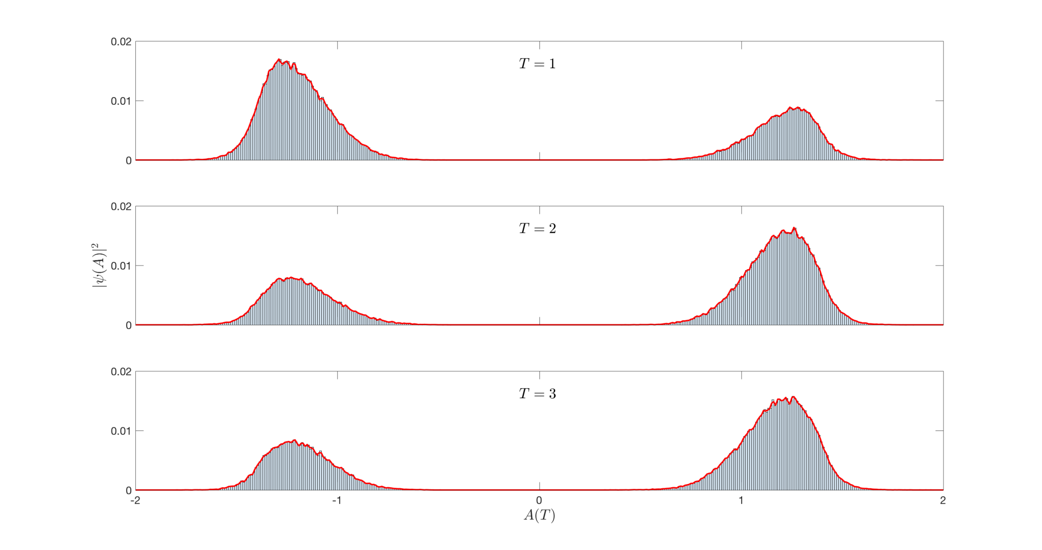
Our main results appear in Fig. 14. This displays plots of the wavefunction with parameters for various values of . The wave function in each case is calculated by binning the final time steps for the subset of paths from the samples that cross the classical turning points at least once. Such paths are deemed to have tunnelled. The total number of samples for each value of was .
The main result here is that our simulation method gives explicit tunnelling wave functions. These appear to be anti-symmetric, with one or the other side favoured. This depends on the initial seed path from which the samples are generated.
VII Summary and discussion
We explored the application of the PIMC method to FLRW quantum cosmology with dust and cosmological constant. Using the dust field as a clock, we solve the Hamiltonian constraint classically, and then proceed with the application of MC algorithms to compute various properties of the model. Our main result is that the MC method with matter time provides a useful alternative for exploring quantum cosmologies, one that can inform analytical semiclassical calculations of wave functions of the Universe.
Our specific results are as follows. (i) For the PIMC algorithm converges to the unique ground state wave function for the model; this permits various calculations, such as volume fluctuations and correlation functions. (ii) For the potential term in the Hamiltonian is not bounded below. This poses a computational challenge. Nevertheless, for the variables we use, the Euclidean path integral is bounded for final time Carreau et al. 1990. Within this bound our results indeed converge; we calculated the no-boundary and tunnelling wave functions. Since the observed value of is close to zero, it is clear that this method permits such calculation for very large times.
We also observed that the alternative method for convergence is to impose a lower bound on the Euclidean action . Here we saw that there is a continuum of degenerate vacua, and the Markov chain terminates in the neighbourhood of one point of this continuum. For this reason this algorithm does not explore all possible configurations. Indeed any system with an that is bounded below, and has a continuum of ground states would face this issue in an MC simulation. Thus, since each such vacuum is highly quantum with distinct physical properties, physical results end up depending on the initial state. In our simulations, we see this dependence on initial state appear, for example, in the calculation of the expectation value of the physical volume as a function of time Fig. 12.
Our approach is readily adapted to include other matter in addition to the dust field. It can also be extended to anisotropic cosmology, where it may prove useful in exploring what becomes of the oscillatory behaviour of scale factors near the singularity. Extending the algorithm to Bianchi I is quite straightforward. Computational cost for a semiclassical analysis would be quite manageable, with three instead of one scale factor paths randomly chosen sufficiently close to a chosen classical path. However, for going beyond semiclassical paths to arbitrary random paths, preliminary simulations indicate that thermalization takes significantly more time. Nevertheless since MC codes are naturally run with parallelization computational cost is not an issue. This work is in progress.
Acknowledgements.
This work was supported by the Natural Science and Engineering Research Council of Canada. S.M.H. was also supported by the Lewis Doctoral Fellowship.References
- Rovelli (2000) C. Rovelli, in Recent developments in theoretical and experimental general relativity, gravitation and relativistic field theories. Proceedings, 9th Marcel Grossmann Meeting, MG’9, Rome, Italy, July 2-8, 2000. Pts. A-C (2000) pp. 742–768, arXiv:gr-qc/0006061 [gr-qc] .
- Carlip et al. (2017) S. Carlip, D.-W. Chiou, W.-T. Ni, and R. Woodard, in One Hundred Years of General Relativity: From Genesis and Empirical Foundations to Gravitational Waves, Cosmology and Quantum Gravity (Volume 2), Vol. Volume 2 (2017) pp. 325–347.
- Hartle and Hawking (1983) J. B. Hartle and S. W. Hawking, Phys. Rev. D28, 2960 (1983).
- Vilenkin (1982) A. Vilenkin, Phys. Lett. 117B, 25 (1982).
- Vilenkin (1986) A. Vilenkin, Phys. Rev. D33, 3560 (1986).
- Halliwell and Louko (1989) J. J. Halliwell and J. Louko, Phys. Rev. D39, 2206 (1989).
- Halliwell and Hartle (1990) J. J. Halliwell and J. B. Hartle, Phys. Rev. D41, 1815 (1990).
- Feldbrugge et al. (2017) J. Feldbrugge, J.-L. Lehners, and N. Turok, Phys. Rev. D95, 103508 (2017), arXiv:1703.02076 [hep-th] .
- Isham (1992) C. J. Isham, in 19th International Colloquium on Group Theoretical Methods in Physics (GROUP 19) Salamanca, Spain, June 29-July 5, 1992 (1992) arXiv:gr-qc/9210011 [gr-qc] .
- Schleich (1990) K. Schleich, Class. Quant. Grav. 7, 1529 (1990).
- Maeda (2015) H. Maeda, Class. Quant. Grav. 32, 235023 (2015), arXiv:1502.06954 [gr-qc] .
- Ali et al. (2018) M. Ali, S. M. Hassan, and V. Husain, Phys. Rev. D98, 086002 (2018), arXiv:1807.03864 [gr-qc] .
- Ambjorn et al. (2010) J. Ambjorn, J. Jurkiewicz, and R. Loll, in Proceedings, Foundations of Space and Time: Reflections on Quantum Gravity: Cape Town, South Africa (2010) pp. 321–337, arXiv:1004.0352 [hep-th] .
- Rideout and Sorkin (2000) D. P. Rideout and R. D. Sorkin, Phys. Rev. D61, 024002 (2000), arXiv:gr-qc/9904062 [gr-qc] .
- Perez (2013) A. Perez, Living Rev. Rel. 16, 3 (2013), arXiv:1205.2019 [gr-qc] .
- Ambjorn et al. (2005) J. Ambjorn, J. Jurkiewicz, and R. Loll, Phys. Rev. Lett. 95, 171301 (2005), arXiv:hep-th/0505113 [hep-th] .
- Glaser and Surya (2016) L. Glaser and S. Surya, Class. Quant. Grav. 33, 065003 (2016), arXiv:1410.8775 [gr-qc] .
- Husain and Pawlowski (2011) V. Husain and T. Pawlowski, Class.Quant.Grav. 28, 225014 (2011), arXiv:1108.1147 [gr-qc] .
- Agullo and Singh (2017) I. Agullo and P. Singh, in Loop Quantum Gravity: The First 30 Years, edited by A. Ashtekar and J. Pullin (WSP, 2017) pp. 183–240, arXiv:1612.01236 [gr-qc] .
- Gattringer and Lang (2010) C. Gattringer and C. B. Lang, Lect. Notes Phys. 788, 1 (2010).
- Berger (1988) B. K. Berger, General Relativity and Gravitation 20, 755 (1988).
- Berger (1989) B. K. Berger, Phys. Rev. D 39, 2426 (1989).
- Berger (1993) B. K. Berger, Phys. Rev. D48, 513 (1993).
- Husain and Pawlowski (2012) V. Husain and T. Pawlowski, Phys.Rev.Lett. 108, 141301 (2012), arXiv:1108.1145 [gr-qc] .
- Ali et al. (2016) M. Ali, V. Husain, S. Rahmati, and J. Ziprick, Class. Quant. Grav. 33, 105012 (2016), arXiv:1512.07854 [gr-qc] .
- Hassan and Husain (2017) S. M. Hassan and V. Husain, Class. Quant. Grav. 34, 084003 (2017), arXiv:1705.00398 [gr-qc] .
- Carreau et al. (1990) M. Carreau, E. Farhi, S. Gutmann, and P. F. Mende, Annals Phys. 204, 186 (1990).
- McCoy (1994) B. M. McCoy, in Statistical mechanics and field theory. Proceedings, 7th Physics Summer School, Canberra, Australia, January 10-28, 1994 (1994) pp. 26–128, arXiv:hep-th/9403084 [hep-th] .
- Louko (1988) J. Louko, Phys. Lett. B202, 201 (1988).
- Knorr and Saueressig (2018) B. Knorr and F. Saueressig, Phys. Rev. Lett. 121, 161304 (2018), arXiv:1804.03846 [hep-th] .
- Vilenkin (1988) A. Vilenkin, Phys. Rev. D37, 888 (1988).
- Vilenkin (1994) A. Vilenkin, Phys. Rev. D50, 2581 (1994), arXiv:gr-qc/9403010 [gr-qc] .