Observability Properties of Colored Graphs
Abstract
A colored graph is a directed graph in which nodes or edges have been assigned colors that are not necessarily unique. Observability problems in such graphs consider whether an agent observing the colors of edges or nodes traversed on a path in the graph can determine which node they are at currently or which nodes were visited earlier in the traversal. Previous research efforts have identified several different notions of observability as well as the associated properties of graphs for which those observability properties hold. This paper unifies the prior work into a common framework with several new results about relationships between those notions and associated graph properties. The new framework provides an intuitive way to reason about the attainable accuracy as a function of lag and time spent observing, and identifies simple modifications to improve the observability of a given graph. We show that one form of the graph modification problem is in NP-Complete. The intuition of the new framework is borne out with numerical experiments. This work has implications for problems that can be described in terms of an agent traversing a colored graph, including the reconstruction of hidden states in a hidden Markov model (HMM).
Index Terms:
Graph theory, graph labeling, Markov processes, weak models, tracking.I Introduction
Consider an agent traversing a directed graph whose nodes (or edges) are assigned one or more colors. The agent seeks to localize itself within the graph based on the colors observed. In such problems, the nodes can represent states, the edges can represent allowed state transitions, and the colors can represent the discrete symbols that can be emitted by a given state (in the case of node-colored graphs) or a given state transition (in the case of edge-colored graphs). Such models are used in a variety of applications, some of which are described in the following section.
We consider various formulations of inferring the nodes and edges visited by an agent when only the sequence of colors emitted can be observed directly. What can be inferred about nodes and edges is collectively called an observability property. Previous work has identified several classes of colored graphs, each having different implications for the tractability and accuracy of this inference problem [1, 2, 3]. Some of the related notions which have arisen in other contexts including symbolic dynamics [4] and discrete event systems [5, 6, 7, 8] are nicely summarized in [3]. The present work unites these concepts in a comprehensive framework based on the presence or absence of particular pathologies in the graph and its coloring. We also provide a unified structure to reason about the effects of specific pathologies and to design mitigations that improve the observability properties of a given graph.
The readers should note that we are not studying the more challenging problem of inferring the graph and its coloring from sequences of color observations which is a different computational problem [9]. In particular, we are assuming that the graph and its coloring are known a priori and not being learned by the observer.
The rest of the paper is structured as follows: Section II describes our notation and reviews the previous work on colored graph models and observability classes. Section III presents the colored graph pathologies and discusses their implications and possible mitigations. Section IV presents the relationships between colored graph observability classes. Section VI illustrates the implications of the various pathologies using simulations. Finally, Section VII summarizes the contributions of this paper and discusses potential directions for future work.
II Background and Previous Work
II-A Definitions: Colored Graphs, Weak Models, and Hidden Markov Models
A node-colored directed graph consists of a set of nodes , a set of edges consisting of ordered pairs of nodes, a set of possible colors , and a mapping which indicates which subset of can be emitted by a given node. This is identical to the definition of a weak model given in [2]. (Note that some authors also include the set of nodes which the system can start at as part of their definition of a weak model [10, 1].)
If each edge is endowed with a transition probability (where is the node visited at time ) and each node is endowed with a set of emission probabilities (where is the color emitted at time and ), the model is a hidden Markov model (HMM) with discrete symbols [11]. Note that we are concerned here with structural properties of such systems that depend only on whether certain state transitions and emissions are possible or not, and not on the specific probabilities. Consequently, our results are about whether certain inferences about colored graphs are true or not true, as opposed to what the probabilities or likelihoods of inferences are.
A node-colored graph is multi-colored if there exists a such that . In the context of tracking an agent traversing the graph, the implication is that one of the possible colors will be emitted when the agent visits node . It is often useful to reduce such a graph to the equivalent single-colored graph. This can be accomplished by replacing every multi-colored node with multiple nodes, one for each color, then duplicating the appropriate edges. This is illustrated in Figure 1.


An edge-colored directed graph is defined as above, but instead associates the mapping to colors with the edges: . As with the node-colored case, it is possible to have an edge-multi-colored graph if there exists an such that . Edge-colored graphs can describe higher-order dependencies (e.g., they represent a system where the color emitted depends on both the current node and the previous node), so it is often useful to reduce an edge-colored graph to an equivalent node-colored graph. This can be accomplished by replacing every node which has incident edges of more than one color by multiple nodes, one for each color, then assigning each node the color of its incident edges. This is illustrated in Figure 2.
Therefore, every node-multi-colored graph and every edge-colored graph, whether multi-colored or not, can be reduced to an equivalent node-colored graph for which each node emits only one color. Moreover, the reduction results in modest growth of the graph. Specifically, if there are nodes in the graph and the multi-colored node or edge with the most colors has colors, the resulting simply colored node graph will have no more than unicolored nodes.
Consequently, in the remainder of this paper, we consider, without loss of generality, node colored graphs for which each node can emit only one color.


II-B Example Applications
Such models have been applied in a variety of contexts. In our previous work in the cybersecurity domain, the nodes are the basic blocks of a software program’s control flow graph (CFG), the edges are the allowed control flow transitions (dictated by jump, call, and return instructions in the program), and the colors are the specific signals emitted in a side-channel (e.g., electromagnetic emissions) [12, 13]. The colored graph model is used to reason about how accurately the program execution can be tracked in order to verify that the software is functioning as expected.
In a different cybersecurity context, colored graph models have been used as part of process query systems to detect attacks on computer networks [14, 15, 16]. Here, the nodes are the states of the attacker as they compromise various elements of the network and the colors are the signals produced by a variety of sensors used to instrument the network as part of its intrusion detection system. In this context it is of interest to determine both which process (or processes, in the case of multiple simultaneous attacks) is running as well as the current state which any given process is in.
Previous work has also applied colored graph models to target tracking in sensor networks [2]. Here the nodes are physical locations, the edges are the allowed movements from location to location, and the colors are the sensor signals. The colored graph formalism allows reasoning about how well a target can be tracked given noisy/ambiguous sensor reports.
II-C Observability Classes
Suppose that an agent is traversing a given node-colored graph, yielding a sequence of observed colors from which we seek to infer something about the underlying state or node sequence that generated those observed colors. A “hypothesis” in the context of such an observability problem is any sequence of nodes that can be visited when traversing a directed path that emits the observed colors .
Applications often distinguish between real-time tracking where we try to find given and a posteriori reconstruction where we try to infer some part (even all) of the sequence of nodes given . In addition, different versions of the problem can make different assumptions about whether the start state is known or not. In general, there is no guarantee that any of the nodes can be unambiguously identified, even a posteriori.
Previous work has identified a number of classes of colored graphs for which guarantees of varying strength can be made, however:
- •
In a trackable graph the number of hypotheses consistent with an observation sequence grows polynomially in the length of the observation sequence [2]. In a graph which is not trackable, the number of hypotheses grows exponentially. It is known that the number of hypotheses can grow either polynomially or exponentially, with no intermediate growth rates possible [2].
- •
In a unifilar graph the current node is unambiguously determined given the previous node and the current color [1]. Furthermore, each node emits exactly one color and each color can be emitted by at most one of the starting nodes. (Thus, the start node is determined unambiguously by the initial observed color.) The implication of these constraints is that there is a one-to-one correspondence between color sequences and node sequences.
- •
In a partly a posteriori observable graph it is possible, given a sufficiently long observation sequence, to unambiguously determine the state at at least one point in the past [3].
- •
In a partly observable graph there is an upper bound, , on how much time there is between opportunities for to be unambiguously determined given the observation sequence , where [3].
- •
In an observable graph, the node can be unambiguously determined given the observation sequence , provided (where is a deterministic burn-in period determined by the structure of the graph) [3].
While the previous work characterized these classes using a variety of approaches and definitions [2, 3, 1], Section IV shows that they can all be expressed in a common framework.
II-D Currency of Estimates
Previous work on indexing systems (e.g., search engines) has characterized the quality of estimates in terms of -currency [17, 18, 19]. Specifically, a quantity which was previously observed at time is said to be -current at time if it has not changed between time and time . The quantity is said to be -current if it is -current with probability .
Appropriately interpreted for the new domain, -currency provides a useful metric for characterizing the properties of the various observability classes. Specifically, when tracking an agent traversing a colored graph, our estimate is said to be -current at time if we can correctly identify the node with probability . Note that this definition does not make reference to the “time of last observation,” , because there are no times at which the node is observed directly. Instead, what matters is how long we have been observing the color sequence: the record length, . Therefore, we say that an estimate is -current if we can correctly identify the node with probability using the observed colors . This is illustrated in Figure 3.
As an example, an observable graph is -current. Because of the coloring constraint on the set of starting nodes, a unifilar graph is -current. Other classes are more complicated; attainable values of , , and depend on the specific structure of the graph.
III Colored Graph Pathologies
III-A Description of the Pathologies
Jungers and Blondel present polynomial-time algorithms to check whether a graph is observable or partly a posteriori observable by checking for the following properties [3]:
- 1.
Presence/absence of nodes which have out-neighbors of the same color.
- 2.
Presence/absence of separated cycles having the same sequence of colors. Two cycles indexed by and permitting the same sequence of colors (i.e., ) are said to be separated if for all steps . (It is possible, however, to have for ; see Figure 4.)
In Section IV-C, we show that the polynomial-time algorithm given by Crespi et al. to check whether a graph is trackable is equivalent to checking for the following additional property [2]:
- 3.
Presence/absence of intersecting cycles having the same sequence of colors. Two cycles , permitting the same sequence of colors are said to be intersecting if there is at least one such that . (We exclude the trivial case of identical cycles where .)

Note that intersecting cycles with the same coloring are a subset of same-colored out-neighbors: because a pair such cycles must intersect, there must be some such that and . (Recall that we exclude identical cycles.) The fact that and are taken to permit the same sequence of colors means that and are same-colored out-neighbors of the branching point . But, as shown by the examples in Figure 6, not all same-colored out-neighbors are part of intersecting cycles with the same coloring.
This enumeration suggests that the three pathologies listed in Table I are useful for characterizing the various observability classes.
Name
Example
Effect
Mitigation
Same-colored out-neighbors
![[Uncaptioned image]](1811.04803v2/figures/scon.png) Lose track, may be able to reconstruct a posteriori, increases for given
Lose track, may be able to reconstruct a posteriori, increases for given
![[Uncaptioned image]](1811.04803v2/figures/scon_mit.png) Intersecting cycles with same coloring
Intersecting cycles with same coloring
![[Uncaptioned image]](1811.04803v2/figures/intcyc.png) Lose track, may never be able to reconstruct, decreases maximum attainable
Lose track, may never be able to reconstruct, decreases maximum attainable
![[Uncaptioned image]](1811.04803v2/figures/intcyc_mit.png) Separated cycles with same coloring
Separated cycles with same coloring
![[Uncaptioned image]](1811.04803v2/figures/sepcyc.png) Increases “burn-in” time before nodes can be reconstructed unambiguously, increases required for a given
Increases “burn-in” time before nodes can be reconstructed unambiguously, increases required for a given
![[Uncaptioned image]](1811.04803v2/figures/sepcyc_mit.png)
In fact, in Section IV we show that these three pathologies are sufficient to describe observable, partly a posteriori observable, trackable, and a looser class of unifilar graphs (i.e., without the constraint on the set of starting nodes). Partly observable graphs do not fit quite as cleanly into this framework as the others, but some cases can be characterized by the absence of a specific type of same-colored out-neighbor described in Section IV-E.
III-B Effects of the Pathologies
In loose terms, the effects of each pathology are:
- •
Same-colored out-neighbors cause tracking to be lost once they are encountered. But, it will often be possible to reconstruct which branch was taken a posteriori. For example, in the top row of Table I, once is seen, we do not know which node the agent is at. But, the next observation will either be (in which case we know the previous step took the left-hand branch) or (in which case we know the previous step took the right-hand branch). Therefore, the net effect on -currency is to increase the lag necessary to obtain a given accuracy . Provided that , the record length will have no effect on the ability to determine which branch was taken.
- •
Intersecting cycles with the same coloring is a special case of same-colored out-neighbors which causes tracking to be lost in a way which can prevent even a posteriori reconstruction of the visited nodes. For example, in the middle row of Table I, the observations will always be an alternating sequence of and , but it will never be possible to determine which of the nodes was visited. Therefore, the net effect on -currency is to decrease the accuracy which can be obtained for any lag or record length .
- •
Separated cycles with the same coloring increase the “burn-in” time for which colors must be observed before a node (past or present) can be identified unambiguously. For example, consider a sequence of observations from the graph in the bottom row of Table I consisting of alternating and . Until is observed, it is not possible to know which side of the graph the agent is on. But, as soon as one of the sequences (, ) or (, ) is observed, we know not only where the agent is, but where it was at all previous times.
When there is no risk of confusion, the words “with the same coloring” will be omitted when referring to intersecting and separated cycles.
III-C Mitigating the Pathologies
Enumerating the pathologies is useful not just to understand their implications, but also to create ways of mitigating their deleterious effects on tracking performance. A simple way to modify a colored graph’s observability class without significantly changing the functionality of the underlying system is to add uniquely-colored but otherwise non-functional “indicator nodes” at strategic locations. These are indicated by the grey hexagons () in the last column of Table I. This approach was demonstrated experimentally in [12], and further simulated examples are given in Section VI.
The basic idea is to insert an indicator node either just before a same-colored out-neighbor or in a cycle with the same coloring in order to remove the pathology. Because the addition of an indicator node causes a delay in the traversal of the graph, it is desirable to put the indicator nodes in parts of the graph which are less-frequently visited. In an HMM, one can determine the long-run frequency of each transition in order to decide where to place indicator nodes.
In principle it is also possible to change the observability class through the deletion of nodes and/or edges, instead of the insertion of nodes into existing edges discussed above. This could correspond to restructuring the system to avoid certain ambiguous behaviors. But, because this will clearly affect the functionality of the system more than the addition of indicator nodes, we do not consider these cases any further here.
IV Pathology-Based Taxonomy of Colored Graph Observability Classes
A taxonomy of colored graph classes based on the presence/absence of the graph pathologies is given in Figure 5. Simple example graphs from each region of the Venn diagram are given in Figure 6. The full reasoning for each class/region is given in the following subsections.


IV-A Region I: General Colored Graphs
The outer part of the Venn diagram is the universe of all possible colored graphs, which may have all of the pathologies represented, and for which no performance guarantees can be made.
IV-B Region II: Partly a Posteriori Observable
A graph is partly a posteriori observable if there are no separated cycles with the same color sequence [3].
To check if a colored graph possesses this property, construct the auxiliary graph whose nodes are of the form , where and . The auxiliary graph contains an edge if , , and and have the same color (i.e., ). If is acyclic, then contains no separated cycles with the same color sequence [3].
IV-C Region III: Trackable
Crespi et al. characterize trackability by considering the node sequences consistent with all possible color sequences [2]. A graph is trackable if and only if, for each possible color sequence, there is at most one path from each node at time back to itself at time which is consistent with the color sequence (this is the “unique path property”). But, if two different paths begin and end at the same node and have the same color sequence, then they form a pair of intersecting cycles with the same coloring. Therefore, the absence of such cycles is a necessary and sufficient condition for a graph to be trackable.
IV-D Region IV: Partly a Posteriori Observable and Trackable
As shown by the example in Figure 6d, it is possible for a graph to lack both separated and intersecting cycles with the same coloring but to not belong to any of the more restrictive classes. Namely, the absence of both separated and intersecting cycles with the same color sequence is not a sufficient condition for a graph to be partly observable. (Nor is it a necessary condition, see Figure 6e.)
IV-E Regions V and VI: Partly Observable
Partial observability is characterized by another auxiliary graph, [3]. To construct , add the edge to if the following three conditions are met:
- 1.
has edge or
- 2.
has edge or
- 3.
and have the same color (i.e., )
A graph is partly observable if is acyclic. Because is a supergraph of , it has at least as many cycles as and hence partly observable is a subset of partly a posteriori observable.
Graphs which are partly a posteriori observable but not partly observable (i.e., is acyclic but is not) appear to be characterized by a specific class of same-colored out-neighbors similar to the example in Figure 6d: there is a cycle connected to a path which permits the same sequence of colors as the cycle, but the path ends at a different node and hence does not form an intersecting cycle. The net effect of this configuration is to permit color sequences of arbitrary length with ambiguous endpoints, thereby violating the conditions for partial observability. Specifically, in Figure 6d, we cannot know in real-time when a sequence of the form (, , , , …) has transitioned from the left-hand branch to the right-hand branch. But, once we see the sequence (, ) twice in a row, we know that the previous two nodes were in the left-hand branch, but remain uncertain about which branch the agent is currently on. Therefore, the net effect of this pathology is simply to increase the lag for correct identification of nodes. Because the effect on -currency is identical to the more general class of same-colored out-neighbors which do not form intersecting cycles, we have chosen to not include this as a specific pathology in Table I, but simply include partly observable as a subset in our taxonomy.
As noted in [3], partly observable graphs may or may not be trackable. We have designated these cases regions V and VI, respectively.
IV-F Region VII: Semi-Unifilar
A graph is unifilar if the following three conditions are met [1]:
- 1.
Each node emits exactly one color: .
- 2.
For each node and each color , there is at most one out-neighbor of which can emit .
- 3.
For each color , the agent can start at at most one node which emits .
Condition 1 is not necessary for the favorable tracking properties of unifilar graphs described in Section II-C. (It is used in [1] to establish bounds on the rate of growth of the set of possible color sequences from weak models.) Condition 2 simply states that there are no same-colored out-neighbors. Our taxonomy does not consider the set of nodes which the agent is permitted to start at, so we do not consider condition 3. Therefore, we call a graph semi-unifilar if it satisfies condition 2 (no same-colored out-neighbors).
Semi-unifilar graphs have the property that, once a node is identified unambiguously, all nodes from then on will also be identified unambiguously. But, semi-unifilar graphs do not have any guarantees that you will be able to perform this initial localization. For example, the graph in Figure 4 is semi-unifilar but, because of its symmetry, it will never be possible to unambiguously identify any nodes without additional information beyond the observed color sequence.
Because intersecting cycles with the same coloring are a specific case of same-colored out-neighbors, semi-unifilar is clearly a subset of trackable. Contradicting the assertion that unifilar graphs are a particular case of observable graphs in Section 1 of [3], we note that unifilar (and semi-unifilar) graphs can have separated cycles with the same coloring, and are therefore in fact a superset of observable graphs. An example of a semi-unifilar graph which is not observable is given in Figure 6g.
IV-G Region VIII: Observable
A graph is observable if it lacks both separated cycles with the same coloring and same-colored out-neighbors [3]. In other words, observable graphs are pathology-free.
V Optimal Indicator Node Placement Is NP-Complete
In this section, we consider the problem of making an arbitrary graph partly a posteriori observable by adding some number of indicator nodes. We show that this problem is in NP-Complete, but leave open the questions of obtaining other observability-type properties through the insertion of indicator nodes. Recall that adding an indicator node means replacing an edge with a new node and new edges and . Table I illustrates the concept with three examples. To be precise, consider the following formulation of the problem.
Indicator Node Selection Problem: Given a node-colored directed graph, , and a subset of edges, , can indicator nodes be added to some edges in so that the resulting graph is partly a posteriori observable?
Theorem 1.
The Indicator Node Selection Problem is in NP-Complete.
The proof is deferred to the Appendix (part of the supplemental material) because the reduction is detailed and would detract from the present narrative. But we note here that the very question of whether inserting indicator nodes into a given subset of edges can make the resulting graph partly observable is in NP-Complete without requiring that the number of added indicator nodes be minimal. Moreover, the proof of Theorem 1 will show that the result is true irrespective of what color the indicator nodes are – they can be one of the existing colors in or an entirely new color.
However, the proof does not address the problem of adding indicator nodes with arbitrary numbers of new colors nor the problem of repeatedly adding indicator nodes to the same original edge because those cases are trivial. To see this, note that every edge in could have a single uniquely colored indicator node color inserted or a unique number of same colored indicator nodes inserted to make each edge effectively uniquely colored.
VI Numerical Experiments: Changing Graph Class With Indicator Nodes
In order to illustrate the effects of the pathologies and mitigations, we have conducted a series of numerical experiments using the graph shown in Figure 7a. This graph has all three pathologies present, and hence is expected to have poor tracking performance.


VI-A Improving Tracking Performance: Trackable and Semi-Unifilar
The base case shown in Figure 7a has a pair of intersecting cycles of the form (, , , , ). These will prevent reconstruction of which nodes were visited: every time the sequence (, ) is observed, the size of the hypothesis set doubles, consistent with the exponential growth expected for an untrackable graph.
To illustrate this, we simulated draws of 50 steps each from an HMM defined by the graph shown in Figure 7a. The probabilities of transitions out of each node were set to be equal, and the nodes were taken to be single-colored. To capture the steady-state behavior, we set the initial state distribution of the HMM to be equal to the equilibrium distribution. We then used the Viterbi algorithm to reconstruct the node sequence from the color sequence with various lags and record lengths .
The accuracy (where and are the predicted and true nodes at time , respectively) is shown in Figure 8a. The median accuracy for the base graph is 78%, and drops to 50% for very short record lengths. The steady-state (i.e., high-) behavior is shown in Figure 9. The tracking accuracy is equally poor at all lags: longer record lengths and/or lags do not help reduce the effects of intersecting cycles with the same coloring.


Now consider the addition of an indicator node to mitigate the intersecting cycles, as shown in Figure 7b. The indicator node was placed just before the central node to preserve the same-colored out-neighbors: the modified graph is trackable, but not semi-unifilar. Tracking accuracy for the modified graph (Figure 8b) is 100% for , but the same-colored out-neighbors cause it to drop to around 79% for .
Next, consider moving the indicator node so it also mitigates the same-colored out-neighbors, as shown in Figure 7c. Tracking accuracy for the modified graph (Figure 8c) is 100% for , but the accuracy drops for the first four time steps recorded because there is no way to determine which branch an initial sequence of came from.
VI-B Reducing Burn-In Time: Observable
The graphs considered above contain a pair of separated cycles of the form (, ) which are expected to increase the burn-in time before states can be identified unambiguously. The stationary distribution for the examples above has most of its mass in the eight nodes, which ends up masking this effect. In order to characterize the effect of separated cycles, we generated another set of realizations, each with 50 time steps. For this experiment the initial state distribution was set to be uniform over the lower four nodes in Figure 7a (i.e., the ones which form the separated cycles with the same coloring).
We start with the semi-unifilar graph in Figure 7c because the effects of the other pathologies have already been shown above. Tracking accuracy for this case is shown in Figure 10a. The accuracy starts out poor for all lags , but gradually improves as the record length increases. The lack of dependence on the lag is expected: the graph is semi-unifilar, so once is observed for the first time unambiguous real-time tracking is guaranteed. Furthermore, because the observations cannot start at any of the nodes, all of the initial states are reconstructed once one of the two sequences (, ) or (, ) is observed.
The real-time () tracking performance is shown in Figure 11. The tracking accuracy for the semi-unifilar graph asymptotically approaches 100%. The time constant of this approach can be controlled by varying the probabilities of transitioning to the node; the same equal probabilities used above were used here.


Now consider the addition of an indicator node into the lower right (, ) cycle, as shown in Figure 7d. The modified graph is observable. Consistent with this, 100% tracking accuracy is obtained after a fixed burn-in period of two time steps (see Figure 10b). For the equal transition probabilities used here, this corresponds to approximately faster burn-in compared to the semi-unifilar case.
VII Conclusions and Future Work
This paper has presented a new pathology-based taxonomy of colored graph observability classes which unifies the results of [1, 2, 3] into a common framework. The three colored graph pathologies identified provide an intuitive picture of the differences between the various observability classes, and the expanded concept of -currency provides a principled way of reasoning about the effects of the various pathologies. Numerical experiments have shown the ability to change the observability class of a graph through the addition of indicator nodes, providing a more complete view of this topic than the initial experimental results in [12]. Furthermore, we have shown that at least one form of the Indicator Node Selection Problem is in NP-Complete. The formulation of the taxonomy has intentionally avoided questions of transition/emission probabilities and initial state distributions so that the results are as general as possible, and hence can be applied to any situation where a hidden state sequence is to be reconstructed from noisy/potentially ambiguous observations.
In terms of possible future research directions, consider the following observations. There is a large well-known literature on problems of graph colorability. Loosely speaking, those problems ask how many colors are required to color nodes in a graph so that no two adjacent nodes have the same color [20]. The classic problem in this area is of course the four color problem for planar graphs.
The “chromatic number” of a graph is the smallest number of colors that make the graph colorable in the above sense. Determining the chromatic number is known to be in NP-complete, and therefore the most efficient algorithms currently known are of exponential complexity [21].
By analogy, we can imagine defining a “p-observability number” of a directed graph as being the smallest number of colors required to make the graph have the p-observability property, where such a p-observability property is one of the observability properties discussed in this paper. Moreover, just as the chromatic polynomial, , is a polynomial with the property that the number of legal classical colorings of graph using colors is precisely (so that the chromatic number of is the smallest for which ), we imagine there might be a “p-observability polynomial” with the similar property for the “p-observability” of a graph. Such a “p-observability polynomial” would inform us about how difficult or easy realizing the “p-observability property” would be for a specific graph.
To illustrate the intuition of how observability relates to chromatic numbers, consider the following construct. Given a directed uncolored graph , create the auxiliary graph for which
| (1) |
and
| (2) |
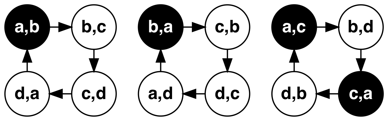
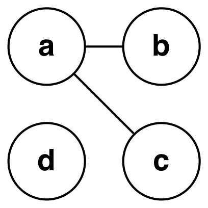
Note that is a supergraph of the auxiliary graph which is used to characterize partly a posteriori observability. In particular, the cycles in are the non-intersecting closed paths of that are potentially indistinguishable from each other. Now select a node from every cycle, , in , which is essentially just a pair of nodes from . Consider the graph with the same nodes as and with edges as selected from the cycles of . is made undirected through inclusion of the edge whenever the edge has been included.
Observe that every traditional coloring of (i.e., no neighboring nodes have the same color) leads to a corresponding coloring of that has no same colored cycles because of how we constructed . Thus the chromatic number of has a clear relationship to the number of ways could be colored to be observable through such a selection of nodes from the cycles in . Note, however, that the construction of is not unique: there can be multiple ways of selecting nodes from the cycles in which lead to different chromatic numbers for . An example of this construction applied to the graph in Figure 4 is given in Figure 12.
This by no means proves anything about any “-observability” polynomial but it does sketch out a concrete relationship between chromatic numbers and observability that could provide insight into future work along these lines.
Acknowledgements
Distribution Statement “A” (Approved for Public Release, Distribution Unlimited)
The research effort depicted was sponsored by the Air Force Research Laboratory (AFRL) and the Defense Advanced Research Projects Agency (DARPA) under the Leveraging the Analog Domain for Security (LADS) program under contract number FA8650-16-C-7622. In particular, we thank Dr. Angelos Keromytis and Mr. Ian Crone, the past and present DARPA program managers of LADS, for their encouragement and support throughout the program.
This research was developed with funding from the Defense Advanced Research Projects Agency (DARPA).
The views, opinions and/or findings expressed are those of the author and should not be interpreted as representing the official views or policies of the Department of Defense or the U.S. Government.
References
- [1] Y. Sheng and G. V. Cybenko, “Distance measures for nonparametric weak process models,” in Systems, Man and Cybernetics, 2005 IEEE International Conference on. IEEE, 2005.
- [2] V. Crespi, G. Cybenko, and G. Jiang, “The theory of trackability with applications to sensor networks,” ACM Transactions on Sensor Networks (TOSN), vol. 4, no. 3, p. 16, 2008.
- [3] R. M. Jungers and V. D. Blondel, “Observable graphs,” Discrete Applied Mathematics, vol. 159, no. 10, pp. 981–989, 2011.
- [4] M.-P. Béal, J. Berstel, S. Eilers, and D. Perrin, “Symbolic dynamics,” Preprint: https://arxiv.org/abs/1006.1265, 2011.
- [5] C. Özveren and A. S. Willsky, “Observability of discrete event dynamic systems,” IEEE Transactions on Automatic Control, vol. 35, no. 7, pp. 797–806, July 1990.
- [6] A. Saboori and C. N. Hadjicostis, “Notions of security and opacity in discrete event systems,” in Proceedings of the 46th IEEE Conference on Decision and Control, 2007, pp. 5056–5061.
- [7] J. Bryans, M. Koutny, L. Mazare, and P. Ryan, “Opacity generalised to transition systems,” International Journal of Information Security, vol. 7, no. 6, pp. 421–435, November 2008.
- [8] A. Saboori, “Verification and enforcement of state-based notions of opacity in discrete event systems,” Ph.D. dissertation, University of Illinois at Urbana-Champaign, 2010.
- [9] M. Kearns and L. Valiant, “Cryptographic limitations on learning boolean formulae and finite automata,” Journal of the ACM (JACM), vol. 41, no. 1, pp. 67–95, 1994.
- [10] G. Jiang, “Weak process models for robust process detection,” in Sensors, and Command, Control, Communications, and Intelligence (C3I) Technologies for Homeland Security and Homeland Defense III, ser. Proc. SPIE, vol. 5403, 2004.
- [11] L. R. Rabiner, “A tutorial on hidden Markov models and selected applications in speech recognition,” Proceedings of the IEEE, vol. 77, no. 2, pp. 257–286, 1989.
- [12] M. Chilenski, G. Cybenko, I. Dekine, P. Kumar, and G. Raz, “Control flow graph modifications for improved RF-based processor tracking performance,” in Cyber Sensing 2018, ser. Proc. SPIE, vol. 10630, 2018, p. 106300I.
- [13] G. Cybenko and G. M. Raz, “Large-scale analogue measurements and analysis for cyber-security,” Data Science For Cyber-security, vol. 3, p. 227, 2018.
- [14] V. Berk and N. Fox, “Process query systems for network security monitoring,” in Sensors, and Command, Control, Communications, and Intelligence (C3I) Technologies for Homeland Security and Homeland Defense IV, ser. Proc. SPIE, vol. 5778, 2005.
- [15] Y. Sheng, “The theory of trackability and robustness for process detection,” Ph.D. dissertation, Dartmouth College, 2006.
- [16] G. Cybenko and V. H. Berk, “Process query systems,” Computer, vol. 40, no. 1, pp. 62–70, January 2007.
- [17] B. E. Brewington and G. Cybenko, “How dynamic is the Web?” Computer Networks, vol. 33, no. 1-6, pp. 257–276, 2000.
- [18] ——, “Keeping up with the changing web,” Computer, vol. 33, no. 5, pp. 52–58, 2000.
- [19] B. E. Brewington, “Observation of changing information sources,” Ph.D. dissertation, Dartmouth College, June 2000.
- [20] T. R. Jensen and B. Toft, Graph Coloring Problems. John Wiley & Sons, 2011, vol. 39.
- [21] M. R. Garey, D. S. Johnson, and L. Stockmeyer, “Some simplified NP-complete graph problems,” Theoretical Computer Science, vol. 1, no. 3, pp. 237–267, 1976.
- [22] M. R. Garey and D. S. Johnson, Computers and Intractability. W.H. Freeman New York, 2002, vol. 29.
| Mark Chilenski received the BS degree in aeronautical and astronautical engineering from the University of Washington in 2010 and the PhD degree in nuclear science and engineering from the Massachusetts Institute of Technology in 2016. He is a senior scientist at Systems & Technology Research LLC. His research interests include machine learning, Bayesian inference, and cybersecurity. |
| George Cybenko received his B.Sc. and Ph.D. degrees in Mathematics from the University of Toronto and Princeton. He is currently the Dorothy and Walter Gramm Professor of Engineering at Dartmouth. His research interests include cyber security, advanced machine learning algorithms and information deception. |
| Isaac Dekine received the BS and MS degrees in electrical and computer engineering from Carnegie Mellon University in 2006. He is a senior engineer at Systems & Technology Research LLC. His research interests include RF system design, signal processing, and cybersecurity. |
| Piyush Kumar received the Master of Science degree in Physics from the Indian Institute of Technology Kharagpur in 2001, MS degree in Physics from the University of Chicago in 2004 and the PhD degree in Physics from the University of Michigan Ann Arbor in 2007. He is a lead scientist at Systems & Technology Research LLC. His research interests include applications of probabilistic methods to problems in physics and engineering, machine learning, and graph theory. |
| Gil Raz received a bachelor’s degree in electrical engineering from the Technion – Israel Institute of Technology in 1988 and a PhD in electrical engineering (minor in mathematics) from the University of Wisconsin – Madison in 1998. He is a chief scientist at Systems & Technology Research LLC. His research interests include applied mathematics and statistics for solving problems in multiple application areas. |
Appendix: Proof of Theorem 1
This appendix provides a proof of Theorem 1. Recall the definition of the Indicator Node Selection Problem from Section V:
Indicator Node Selection Problem: Given a node-colored directed graph, , and a subset of edges, , can indicator nodes be added to some edges in so that the resulting graph is partly a posteriori observable?
Using this definition, we can then state the following theorem:
Theorem 1.
The Indicator Node Selection Problem is in NP-Complete.
Proof.
The idea for the reduction used here was inspired by earlier work showing that edge coloring a graph to make it partly observable with a minimal number of colors is in NP-Complete [3].
Our proof is also based on a reduction from the Monochromatic-Triangle Problem which is known to be in NP-Complete [22] but uses a different reduction mapping. The Monochromatic-Triangle Problem takes as input an undirected graph, , and asks whether there exists a two-coloring of the edges in so that no triangle in has all edges the same color (that is, no triangle is monochromatic).
We will develop the argument based on several steps. Each step involves a stage in the construction of a directed node-colorable graph from with the property that there is a positive answer to the Indicator Node Selection Problem for if and only if can be edge two-colored so that no triangle has all edges the same color.
Step 1: Start by enumerating all triangles in , say , and creating nodes in for each triangle. Label these nodes by the triangle they represent. Next, for each edge in create a unique pair of nodes in and a directed edge between those nodes. We call these edges “real edges.”
Then for each triangle node add a directed edge to the tails of the node-edge combinations created for each of its three edges. We call these edges “connector” edges.
A depiction of this construct is shown in Figure 13 for one triangle and Figure 14 for two triangles. These figures also show the insertion of an indicator node on one of the “real triangle edges.” This indicator node is a surrogate for coloring the corresponding edge in . Note that the underlying can be edge two-colored so that no triangle has all edges the same color if and only if not all three real edges either have or do not have an indicator node inserted. The example constructs in Figures 13 and 14 indicate that at least triangle has one edge colored differently from the other two edges.
Note that this construct is polynomial in the size of .


Step 2: For each triangle , create two additional copies of that triangle node resulting in a total of three copies, , with those copies all pointing to to the starts of the “real edges” in the underlying triangle.

A depiction of this construct is shown in Figure 15. Note that this part of the construct is still polynomial in the size of .
The edges in this constructed graph together with the corresponding graphs constructed for all other triangles in form the subset of the ultimate graph which are candidates for insertion of indicator nodes. Figure 15 shows two edges having indicator nodes, as an example.
Now consider the paths between the three nodes corresponding to a single triangle in and the nodes at the bottom of the real edges, labelled and in Figure 15, for triangle . Each path starts with a connector edge followed by a real edge. These edges can have indicator nodes on them or not.
The fundamental observation that is key for this reduction is that if all three real edges of are colored the same (that is, all have indicator nodes or none have indicator nodes) then there are two disjoint paths from two of the to two of the nodes and , for any combination of indicator nodes on the connector edges, that have the same combination of indicator nodes.
Said another way, if all real edges either have or do not have indicator nodes, then there are two indistinguishable paths from two distinct triangle copy nodes, , to two distinct . To see this, consider the three paths from each to going straight down in Figure 15. Because all real edges are the same in terms of indicator nodes, there are only two possibilities for the connector edges but there are three paths. So at least two of these paths must have the same arrangement of indicator nodes.
Conversely, if we have a triangle in which at least one, but not all, real edges have an indicator node, then we can assign indicator nodes on the connector edges so that a unique can be identified by any path from any of the down. For example, Figure 16 shows such an assignment.

Step 3: Now that we have constructed the subgraph which arises in the Indicator Node Selection Problem, we need to construct the rest of the graph so that indicator nodes can be assigned to to make the overall graph partly observable if and only if the edges in the underlying can be two-colored so that no triangle in has all edges the same color.
Recall that has triangles. Construct a binary tree that has leaves with a node coloring such that a left node child is colored black and a right node child is colored white and the paths from root to leaves are all the same length. This can be done simply by creating a binary tree with leaves and using only of the leaves.
Now make a one-to-one assignment of the leaves in the tree to the triangles in . A node color sequence from the root of the tree to a leaf uniquely identifies a triangle in . Create three copies of this tree and connect leaves to the three copies of the triangle nodes.
Note that a node color sequence from the root of any tree down to the triangle nodes uniquely identifies (which triangle is at the leaf) but not (which copy of that triangle).

Step 4: The final step involves connecting the bottom nodes in to the roots of the three trees. For this, create two separate linear arrays starting with white nodes followed by black nodes. Connect the bottom nodes to start of each of the linear arrays and the end nodes of the linear arrays to each of the three tree copies. This construct is depicted in Figure 17.
Now consider a path through this constructed and observe the colors which are either black or white along the path. When we see a sequence of whites followed by blacks, we know we just traversed one of the linear arrays on the left of Figure 17 because that is the only place where such a color sequence can occur.
After the blacks, we enter one of the three binary trees but we do not know which one of the trees. We traverse the tree and because we know there are edges on all paths in all trees, we know when we reach one of the triangle nodes and which triangle because of the binary encoding but we do not know which one of the three triangle nodes we have reached because we do not know which copy of the tree we traversed.
Recall that we constructed in such a way that if all real edges of a triangle either all have indicator nodes or none have indicator nodes, then there are must be two disjoint paths from two of the to two of the nodes for that triangle that are identically colored. We close those disjoint paths by passing to two different linear arrays and then passing from the linear arrays to the two trees corresponding to the two triangle node copies that started the disjoint paths identified above.
This creates two separated cycles with the same coloring and shows that any assignment of indicator nodes to edges within that results in all three real edges of any triangle being the same means that the resulting is not partly a posteriori observable.
Moreover, an assignment of indicator nodes to for which all real edges of a triangle in have indicator nodes or not means that all edges of that triangle in are colored the same.
On the other hand, suppose that the constructed graph has an assignment of indicator nodes to the edges in that makes partly a posteriori observable. This means that all same colored paths must eventually intersect which in turn implies that not all three real edges corresponding to any triangle in can all have indicator nodes or not. That implies that the original graph can have edges colored so that no triangle has all edges the same color.
This completes the proof of Theorem 1. ∎